
Color-Sensitive Sensor Array Combined with Machine Learning for Non-Destructive Detection of AFB1 in Corn Silage

 , ,
, ,
Abstract
1. Introduction
2. Materials and Methods
2.1. Sample Acquisition
2.2. Preparation of CSAs
2.3. Spectral Data Acquisition from Color-Sensitive Sensor Array
2.4. Determination of AFB1 Content in Silage Corn Feed
2.5. Spectral Data Preprocessing
2.6. Data Preprocessing, Feature Selection, and Model Establishment Algorithms
2.7. Quantitative Forecasting Model Evaluation Metrics
3. Analysis of Test Results
3.1. AFB1 Content Analysis
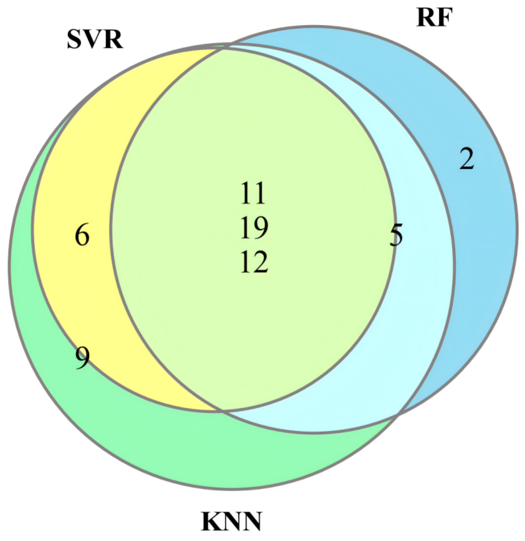
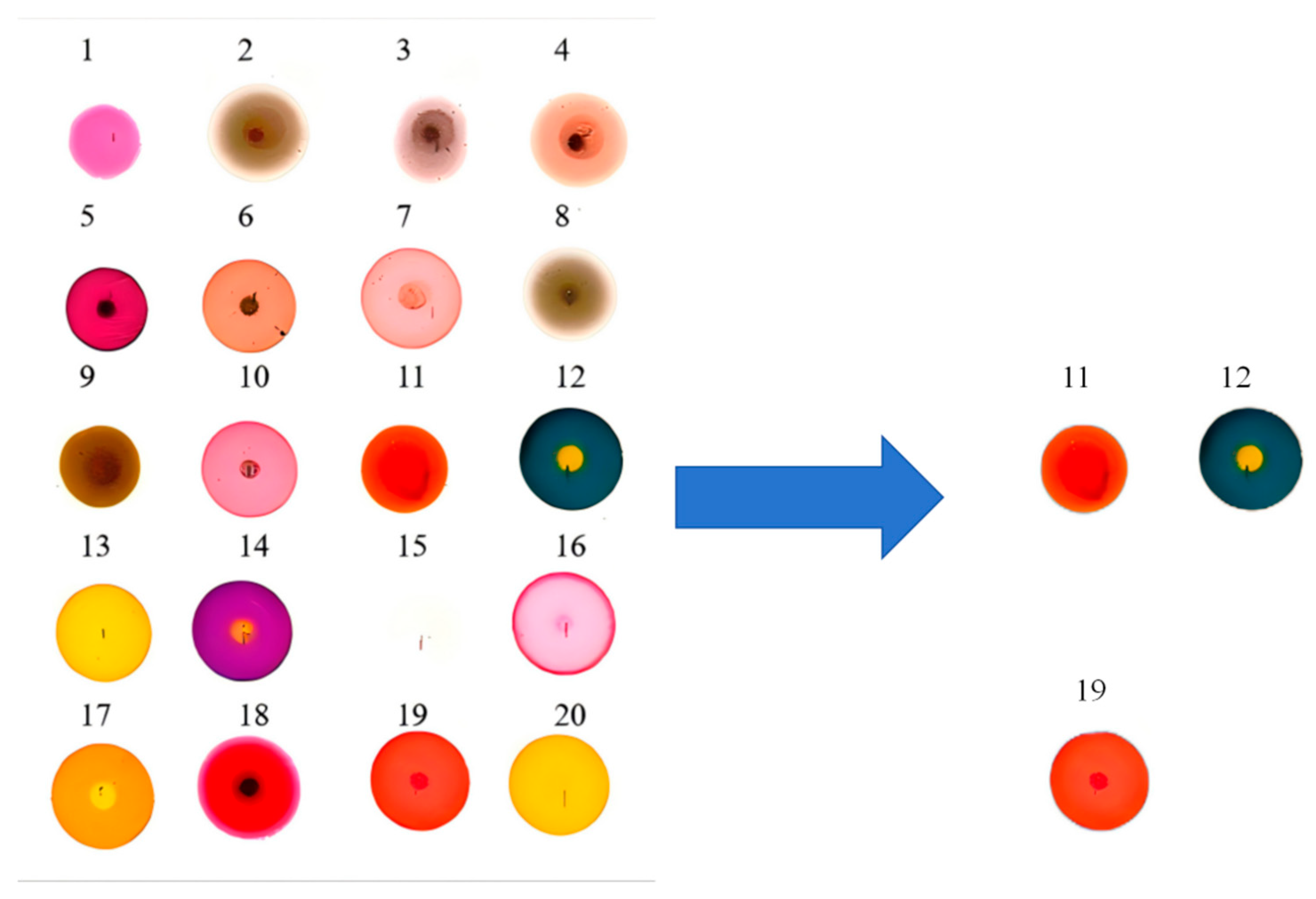
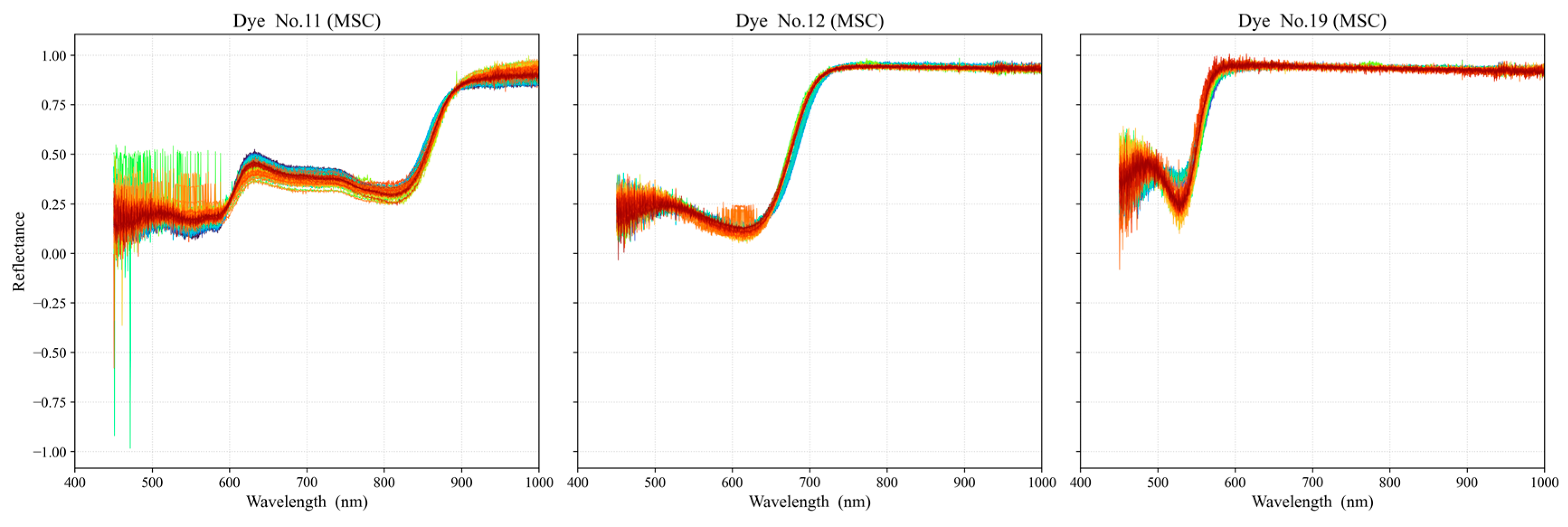
3.2. Data Preprocessing and Selection of Optimal Dye Points
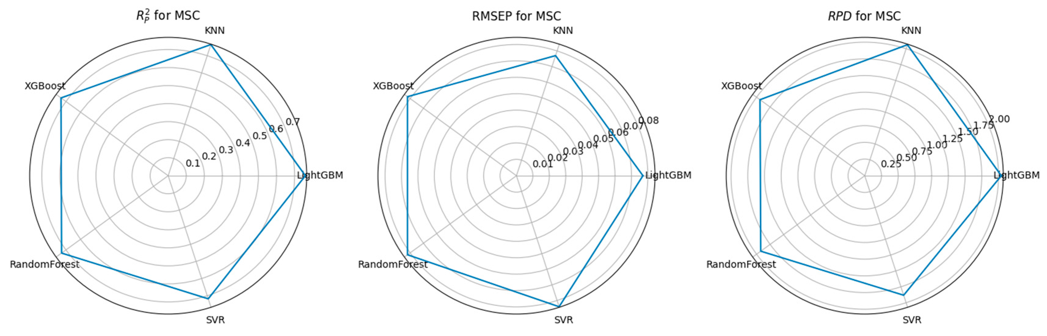
3.3. Feature Selection Algorithms and Determination of the Optimal Model
4. Discussion
4.1. Performance Comparison of CARS-Based Feature Selection Under Stepwise Preprocessing Strategies
4.2. Performance Comparison of PCA-Based Feature Selection Under Stepwise Preprocessing Strategies
4.3. Performance Comparison of KNN-Based Feature Importance Screening Under a Stepwise Preprocessing Strategy
5. Conclusions
Author Contributions
Funding
Institutional Review Board Statement
Data Availability Statement
Conflicts of Interest
Abbreviations
| CSAs | Color-sensitive arrays |
| SNV | Standard Normal Variate |
| MSC | Multiplicative Scatter Correction |
| 1st D | First-order derivative |
| 2nd D | Second-order derivative |
| SVR | Support Vector Regression |
| RF | Random Forest |
| KNN | K-Nearest Neighbor |
| (Mn(OEP)Cl) | (2,3,7,8,12,13,17,18-octaethylporphynato)chloromanganese(III) |
| CARS | Competitive Adaptive Reweighted Sampling |
| PCA | Principal Component Analysis |
| UVE | Uninformative Variable Elimination |
| XGBoost | eXtreme Gradient Boosting |
| LightGBM | Light Gradient Boosting Machine |
| SVM | Support Vector Machine |
| ANN | Artificial neural network |
| LDA | Linear Discriminant Analysis |
| AFB1 | Aflatoxin B1 |
| SWIR | Short-Wave Infrared |
| PSO | Particle Swarm Optimization |
| CMW | Combined Moving Window |
| WD | Wavelet denoising |
References
- Keady, T.W.J.; Hanrahan, J.P. Effects of grass and maize silage feed value, offering soybean meal with maize silage, and concentrate feed level in late pregnancy, on ewe and lamb performance. Animal 2021, 15, 100068. [Google Scholar] [CrossRef] [PubMed]
- Pereira, C.S.; Cunha, S.C.; Fernandes, J.O. Prevalent Mycotoxins in Animal Feed: Occurrence and Analytical Methods. Toxins 2019, 11, 290. [Google Scholar] [CrossRef] [PubMed]
- Guo, L.; Tian, H.; Wan, D.; Yu, Y.; Zhao, K.; Zheng, X.; Li, H.; Sun, J. Detection of Aflatoxin B1 in Maize Silage Based on Hyperspectral Imaging Technology. Agriculture 2025, 15, 1023. [Google Scholar] [CrossRef]
- Luo, S.; Du, H.; Kebede, H.; Liu, Y.; Xing, F. Contamination status of major mycotoxins in agricultural product and food stuff in Europe. Food Control 2021, 127, 108120. [Google Scholar] [CrossRef]
- Li, Z.; Yang, C.; Lu, W.; Chu, Z.; Zhang, J.; Li, M.; Wang, Q. Ultrasensitive immuno-PCR for detecting aflatoxin B1 based on magnetic separation and barcode DNA. Food Control 2022, 138, 109028. [Google Scholar] [CrossRef]
- Liu, Y.; Huang, J.; Li, M.; Chen, Y.; Cui, Q.; Lu, C.; Wang, Y.; Li, L.; Xu, Z.; Zhong, Y.; et al. Rapid identification of the green tea geographical origin and processing month based on near-infrared hyperspectral imaging combined with chemometrics. Spectrochim. Acta Part A 2022, 267, 120537. [Google Scholar] [CrossRef]
- Tyska, D.; Mallmann, A.O.; Vidal, J.K.; de Almeida, C.A.A.; Gressler, L.T.; Mallmann, C.A.; Gupta, V. Multivariate method for prediction of fumonisins B1 and B2 and zearalenone in Brazilian maize using Near Infrared Spectroscopy (NIR). PLoS ONE 2021, 16, e0244957. [Google Scholar] [CrossRef]
- Correa, J.A.F.; Orso, P.B.; Bordin, K.; Hara, R.V.; Luciano, F.B. Toxicological effects of fumonisin B1 in combination with other Fusarium toxins. Food Chem. Toxicol. 2018, 121, 483–494. [Google Scholar] [CrossRef]
- Levasseur-Garcia, C. Updated Overview of Infrared Spectroscopy Methods for Detecting Mycotoxins on Cereals (Corn, Wheat, and Barley). Toxins 2018, 10, 38. [Google Scholar] [CrossRef]
- Wu, Q.; Xie, L.; Xu, H. Determination of toxigenic fungi and aflatoxins in nuts and dried fruits using imaging and spectroscopic techniques. Food Chem. 2018, 252, 228–242. [Google Scholar] [CrossRef]
- Acuna-Gutierrez, C.; Schock, S.; Jimenez, V.M.; Müller, J. Detecting fumonisin B1 in black beans (Phaseolus vulgaris L.) by near-infrared spectroscopy (NIRS). Food Control 2021, 130, 108335. [Google Scholar] [CrossRef]
- Shen, F.; Huang, Y.; Jiang, X.; Fang, Y.; Li, P.; Liu, Q.; Hu, Q.; Liu, X. On-line prediction of hazardous fungal contamination in stored maize by integrating Vis/NIR spectroscopy and computer vision. Spectrochim. Acta Part A Mol. Biomol. Spectrosc. 2020, 229, 118012. [Google Scholar] [CrossRef]
- Zheng, S.Y.; Wei, Z.S.; Li, S.; Zhang, S.J.; Xie, C.F.; Yao, D.S.; Liu, D.L. Near-infrared reflectance spectroscopy-based fast versicolorin A detection in maize for early aflatoxin warning and safety sorting. Food Chem. 2020, 332, 127419. [Google Scholar] [CrossRef]
- Putthang, R.; Sirisomboon, P.; Sirisomboon, C.D. Shortwave Near-Infrared Spectroscopy for Rapid Detection of Aflatoxin B1 Contamination in Polished Rice. J. Food Prot. 2019, 82, 796–803. [Google Scholar] [CrossRef] [PubMed]
- Li, Z.; Tang, X.; Shen, Z.; Yang, K.; Zhao, L.; Li, Y. Comprehensive comparison of multiple quantitative near-infrared spectroscopy models for Aspergillus flavus contamination detection in peanut. J. Sci. Food Agric. 2019, 99, 5671–5679. [Google Scholar] [CrossRef] [PubMed]
- Kim, Y.-K.; Baek, I.; Lee, K.-M.; Kim, G.; Kim, S.; Kim, S.-Y.; Chan, D.; Herrman, T.J.; Kim, N.; Kim, M.S. Rapid Detection of Single- and Co-Contaminant Aflatoxins and Fumonisins in Ground Maize Using Hyperspectral Imaging Techniques. Toxins 2023, 15, 472. [Google Scholar] [CrossRef] [PubMed]
- Ghilardelli, F.; Barbato, M.; Gallo, A. A Preliminary Study to Classify Corn Silage for High or Low Mycotoxin Contamination by Using near Infrared Spectroscopy. Toxins 2022, 14, 323. [Google Scholar] [CrossRef]
- Hetta, M.; Mussadiq, Z.; Wallsten, J.; Halling, M.; Swensson, C.; Geladi, P. Prediction of nutritive values, morphology and agronomic characteristics in forage maize using two applications of NIRS spectrometry. Acta Agric. Scand. Sect. B Soil Plant Sci. 2017, 67, 326–333. [Google Scholar] [CrossRef]
- Zhao, K.; Tian, H.; Ren, X.; Yu, Y.; Guo, L.; Li, Y.; Tao, Y.; Liu, F. Screening of key volatile compounds characterizing the deterioration of maize silage during aerobic exposure. Rev. Bras. Zootec. 2024, 53, e20230042. [Google Scholar] [CrossRef]
- Wang, J.; Jiang, H.; Chen, Q. High-precision recognition of wheat mildew degree based on colorimetric sensor technique combined with multivariate analysis. Microchem. J. 2021, 168, 106468. [Google Scholar] [CrossRef]
- Ottoboni, M.; Pinotti, L.; Tretola, M.; Giromini, C.; Fusi, E.; Rebucci, R.; Grillo, M.; Tassoni, L.; Foresta, S.; Gastaldello, S.; et al. Combining E-Nose and Lateral Flow Immunoassays (LFIAs) for Rapid Occurrence / Co-Occurrence Aflatoxin and Fumonisin Detection in Maize. Toxins 2018, 10, 416. [Google Scholar] [CrossRef]
- Leggieri, M.C.; Mazzoni, M.; Fodil, S.; Moschini, M.; Bertuzzi, T.; Prandini, A.; Battilani, P. An electronic nose supported by an artificial neural network for the rapid detection of aflatoxin B1 and fumonisins in maize. Food Control 2021, 123, 107722. [Google Scholar] [CrossRef]
- Chen, Z.; Lin, H.; Wang, F.; Adade, S.Y.-S.S.; Peng, T.; Chen, Q. Discrimination of toxigenic and non-toxigenic Aspergillus flavus in wheat based on nanocomposite colorimetric sensor array. Food Chem. 2024, 430, 137048. [Google Scholar] [CrossRef] [PubMed]
- Andueza, D.; Picard, F.; Martin-Rosset, W.; Aufrère, J. Near-Infrared Spectroscopy Calibrations Performed on Oven-Dried Green Forages for the Prediction of Chemical Composition and Nutritive Value of Preserved Forage for Ruminants. Appl. Spectrosc. 2016, 70, 1321–1327. [Google Scholar] [CrossRef]
- Sheini, A. Colorimetric aggregation assay based on array of gold and silver nanoparticles for simultaneous analysis of aflatoxins, ochratoxin and zearalenone by using chemometric analysis and paper based analytical devices. Microchim. Acta 2020, 187, 167. [Google Scholar] [CrossRef]
- Kim, Y.-K.; Baek, I.; Lee, K.-M.; Qin, J.; Kim, G.; Shin, B.K.; Chan, D.E.; Herrman, T.J.; Cho, S.-K.; Kim, M.S. Investigation of reflectance, fluorescence, and Raman hyperspectral imaging techniques for rapid detection of aflatoxins in ground maize. Food Control 2022, 132, 108479. [Google Scholar] [CrossRef]
- Deng, J.; Jiang, H.; Chen, Q. Characteristic wavelengths optimization improved the predictive performance of near-infrared spectroscopy models for determination of aflatoxin B1 in maize. J. Cereal Sci. 2022, 105, 103474. [Google Scholar] [CrossRef]
- Tharangani, R.; Yakun, C.; Zhao, L.; Ma, L.; Liu, H.; Su, S.; Shan, L.; Yang, Z.; Kononoff, P.; Weiss, W.P.; et al. Corn silage quality index: An index combining milk yield, silage nutritional and fermentation parameters. Anim. Feed. Sci. Technol. 2021, 273, 114817. [Google Scholar] [CrossRef]
- Ji, R.; Ma, S.; Yao, H.; Han, Y.; Yang, X.; Chen, R.; Yu, Y.; Wang, X.; Zhang, D.; Zhu, T.; et al. Multiple kinds of pesticide residue detection using fluorescence spectroscopy combined with partial least-squares models. Appl. Opt. 2020, 59, 1524–1528. [Google Scholar] [CrossRef]
- Qian, L.; Daren, L.; Qingliang, N.; Danfeng, H.; Liying, C. Non-destructive monitoring of netted muskmelon quality based on its external phenotype using Random Forest. PLoS ONE 2019, 14, e0221259. [Google Scholar] [CrossRef]
- Tan, K.; Ma, W.; Wu, F.; Du, Q. Random forest-based estimation of heavy metal concentration in agricultural soils with hyperspectral sensor data. Environ. Monit. Assess. 2019, 191, 446. [Google Scholar] [CrossRef] [PubMed]
- Pullanagari, R.R.; Kereszturi, G.; Yule, I. Integrating Airborne Hyperspectral, Topographic, and Soil Data for Estimating Pasture Quality Using Recursive Feature Elimination with Random Forest Regression. Remote Sens. 2018, 10, 1117. [Google Scholar] [CrossRef]
- Nie, J.; Wen, X.; Niu, X.; Chu, Y.; Chen, F.; Wang, W.; Zhang, D.; Hu, Z.; Xiao, J.; Guo, L. Identification of different colored plastics by laser-induced breakdown spectroscopy combined with neighborhood component analysis and support vector machine. Polym. Test. 2022, 112, 107624. [Google Scholar] [CrossRef]
- He, Q.P.; Wang, J. Fault detection using the k-nearest neighbor rule for semiconductor manufacturing processes. IEEE Trans. Semicond. Manuf. 2007, 20, 345–354. [Google Scholar] [CrossRef]
- Zhao, K.; Tian, H.; Zhang, J.; Wan, D.; Xiao, Z.; Zhuo, C. Adaptive fusion of visible-near infrared spectroscopy and colorimetric sensor array using the slime mold algorithm and stacking ensemble: Application in silage quality detection. Measurement 2025, 247, 116785. [Google Scholar] [CrossRef]
- Zhao, K.; Tian, H.; Zhang, J.; Guo, L.; Yu, Y.; Li, H. Adaptive modeling method integrating slime mould algorithm and cascade ensemble: Nondestructive detection of silage quality under VIS-NIRS. Comput. Electron. Agric. 2025, 234, 110247. [Google Scholar] [CrossRef]
- Zhang, Y.; Li, D.; Wang, X.; Lin, Y.; Zhang, Q.; Chen, X.; Yang, F. Fermentation quality and aerobic stability of mulberry silage prepared with lactic acid bacteria and propionic acid. Anim. Sci. J. 2019, 90, 513–522. [Google Scholar] [CrossRef]
- Xue, X.; Tian, H.; Zhao, K.; Yu, Y.; Zhuo, C.; Xiao, Z.; Wan, D. Non-Destructive Detection of pH Value During Secondary Fermentation of Maize Silage Using Colorimetric Sensor Array Combined with Hyperspectral Imaging Technology. Agronomy 2025, 15, 285. [Google Scholar] [CrossRef]


| Number | Name |
|---|---|
| 1 | 2,3,7,8,12,13,17,18-Octaethyl-21H,23H-porphine |
| 2 | 5,10,15,20-Tetrakis(4-methoxyphenyl)-21H,23H-porphine iron (III) chloride |
| 3 | 5,10,15,20-Tetrakis(4-methoxyhenyl)-21H,23H-porphine |
| 4 | 5,10,15,20-Tetrakis(4-methoxyhenyl)-21H,23H-porphine cobalt (II) |
| 5 | 5,10,15,20-Tetraphenyl-21H,23H-porphine |
| 6 | 5,10,15,20-Tetraphenyl-21H,23H-porphine zinc |
| 7 | 5,10,15,20-Tetraphenyl-21H,23H-porphine copper (II) |
| 8 | 5,10,15,20-Tetraphenyl-21H,23H-porphine iron (III) chloride |
| 9 | 5,10,15,20-Tetraphenyl-21H,23H-porphine manganese(III) chloride |
| 10 | 5,10,15,20-Tetraphenyl-21H,23H-porphine palladium(II) |
| 11 | (2,3,7,8,12,13,17,18-octaethylporphynato)chloromanganese(III) |
| 12 | Bromocresol Green |
| 13 | Bromothymol Blue |
| 14 | Bromophenol blue |
| 15 | Congo red |
| 16 | Methyl Red—Ethanol |
| 17 | Bromocresol Purple |
| 18 | Neutral Red |
| 19 | Cresol Red |
| 20 | Bromothymol Blue |
| Model | Preprocessing Methods | Calibration | Prediction | |||
|---|---|---|---|---|---|---|
| RMSEC | RMSEP | RPD | ||||
| SVR | Raw Data | 0.8556 | 0.0547 | 0.7321 | 0.0766 | 1.9427 |
| SNV | 0.9076 | 0.0436 | 0.7674 | 0.0712 | 2.0952 | |
| MSC | 0.9077 | 0.0435 | 0.7688 | 0.0710 | 2.1041 | |
| 1st D | 0.8995 | 0.0455 | 0.6391 | 0.0886 | 1.6849 | |
| 2nd D | 0.9000 | 0.0454 | 0.4847 | 0.1062 | 1.4013 | |
| WD | 0.8215 | 0.0608 | 0.7144 | 0.0790 | 1.8814 | |
| SNV+1st D | 0.8982 | 0.0457 | 0.6819 | 0.0832 | 1.7951 | |
| MSC+WD | 0.9070 | 0.0438 | 0.7531 | 0.0733 | 2.0413 | |
| RF | Raw Data | 0.9287 | 0.0385 | 0.7580 | 0.0729 | 2.0329 |
| SNV | 0.9368 | 0.0362 | 0.7804 | 0.0694 | 2.1339 | |
| MSC | 0.9669 | 0.0262 | 0.8217 | 0.0626 | 2.3682 | |
| 1st D | 0.9461 | 0.0335 | 0.6361 | 0.0894 | 1.6577 | |
| 2nd D | 0.8834 | 0.0492 | 0.3677 | 0.1178 | 1.2576 | |
| WD | 0.9303 | 0.0381 | 0.7440 | 0.0750 | 1.9763 | |
| SNV+1st D | 0.9394 | 0.0355 | 0.7430 | 0.0751 | 1.9724 | |
| MSC+WD | 0.9450 | 0.0338 | 0.7898 | 0.0679 | 2.1811 | |
| KNN | Raw Data | 0.9993 | 0.0264 | 0.7010 | 0.0733 | 1.8289 |
| SNV | 0.9993 | 0.0264 | 0.8425 | 0.0532 | 2.5197 | |
| MSC | 0.9993 | 0.0264 | 0.8103 | 0.0584 | 2.2962 | |
| 1st D | 0.9993 | 0.0264 | 0.8662 | 0.0472 | 2.8420 | |
| 2nd D | 0.9993 | 0.0264 | 0.6805 | 0.0758 | 1.7690 | |
| WD | 0.9993 | 0.0264 | 0.7014 | 0.0733 | 1.8300 | |
| SNV+1st D | 0.9993 | 0.0264 | 0.8326 | 0.0549 | 2.4441 | |
| MSC+WD | 0.9993 | 0.0264 | 0.8013 | 0.0598 | 2.2436 | |
| Model | Dye Point | Method | RPD | |
|---|---|---|---|---|
| SVR | 19 | MSC | 0.7688 | 2.1041 |
| 12 | MSC+WD | 0.6868 | 1.7880 | |
| 11 | MSC | 0.6629 | 1.7256 | |
| RF | 19 | MSC | 0.8217 | 2.3682 |
| 12 | MSC | 0.6779 | 1.7621 | |
| 11 | WD | 0.6971 | 1.8169 | |
| KNN | 19 | 1st D | 0.8662 | 2.8420 |
| 12 | SNV | 0.7839 | 2.1513 | |
| 11 | 1st D | 0.7695 | 2.0827 |
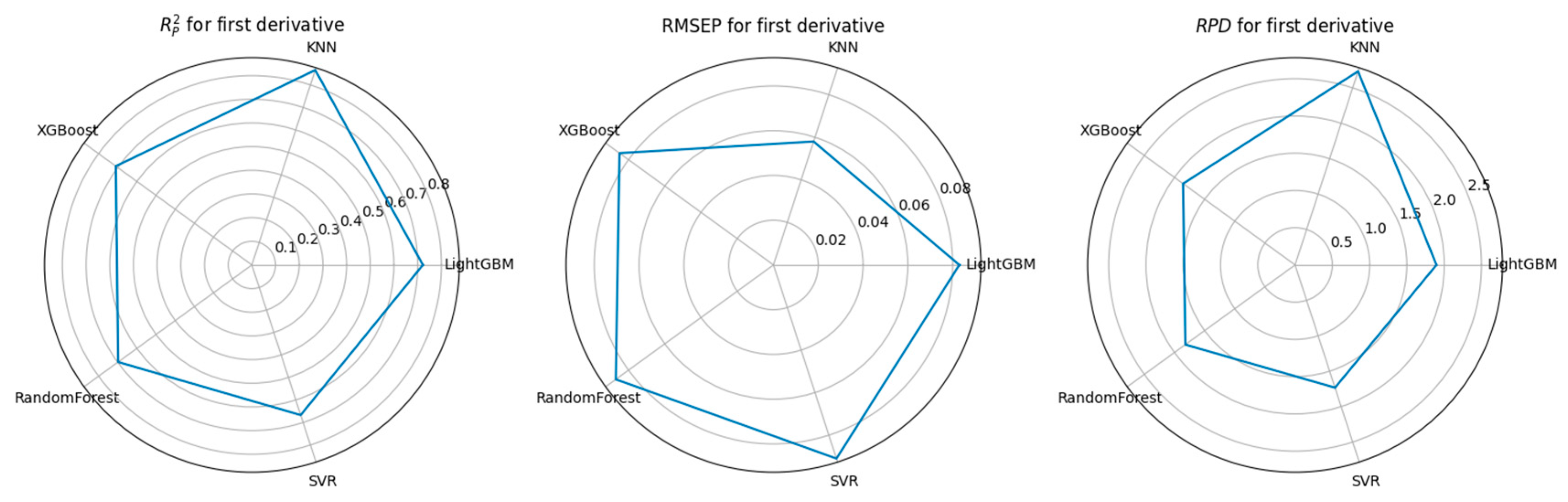
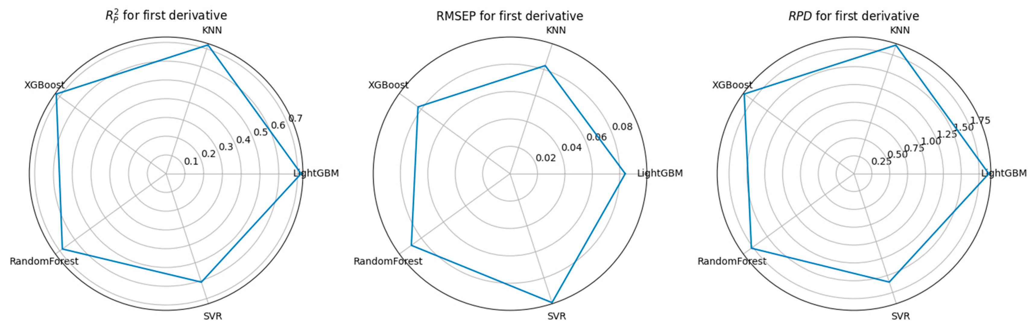
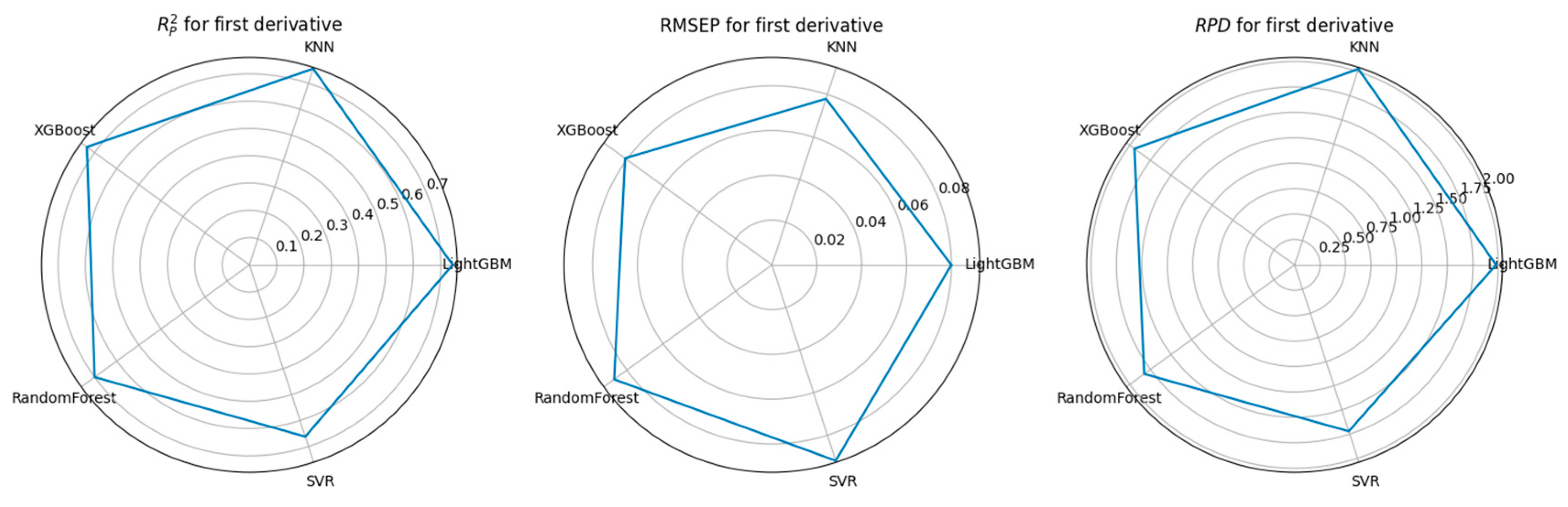
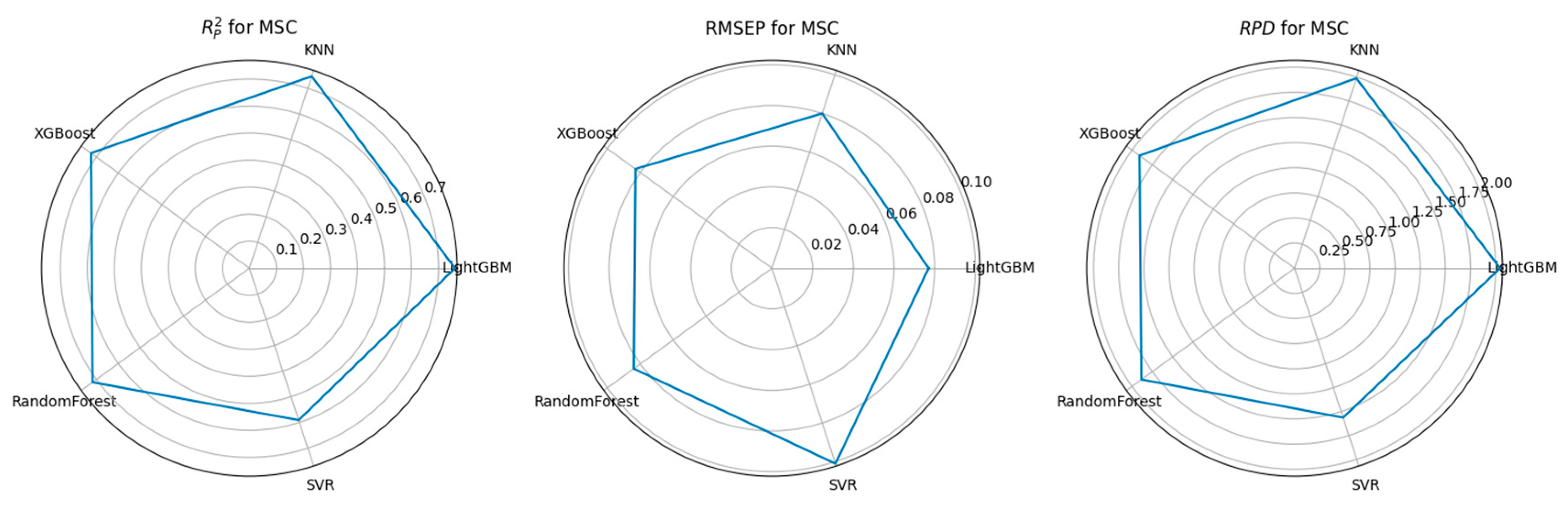
| Feature Selection Algorithm | Preprocessing Methods | Number of Best Features (Where PCA Refers to the Number of Principal Components | Model | RMSEP | RPD | |
|---|---|---|---|---|---|---|
| CARS | MSC | 1001 | LightGBM | 0.76 | 0.077 | 2.042 |
| KNN | 0.765 | 0.077 | 2.063 | |||
| XGBoost | 0.734 | 0.082 | 1.937 | |||
| RF | 0.73 | 0.082 | 1.923 | |||
| SVR | 0.718 | 0.084 | 1.882 | |||
| 1st D | 218 | LightGBM | 0.722 | 0.083 | 1.896 | |
| KNN | 0.866 | 0.058 | 2.733 | |||
| XGBoost | 0.71 | 0.085 | 1.857 | |||
| RF | 0.698 | 0.087 | 1.82 | |||
| SVR | 0.667 | 0.091 | 1.733 | |||
| PCA | MSC | 76 | LightGBM | 0.758 | 0.078 | 2.031 |
| KNN | 0.782 | 0.074 | 2.141 | |||
| XGBoost | 0.695 | 0.087 | 1.812 | |||
| RF | 0.727 | 0.083 | 1.915 | |||
| SVR | 0.721 | 0.084 | 1.892 | |||
| 1st D | 67 | LightGBM | 0.652 | 0.093 | 1.696 | |
| KNN | 0.87 | 0.057 | 2.773 | |||
| XGBoost | 0.58 | 0.102 | 1.544 | |||
| RF | 0.564 | 0.104 | 1.515 | |||
| SVR | 0.706 | 0.086 | 1.844 | |||
| RF | MSC | 792 | LightGBM | 0.757 | 0.078 | 2.029 |
| KNN | 0.779 | 0.074 | 2.128 | |||
| XGBoost | 0.744 | 0.08 | 1.977 | |||
| RF | 0.718 | 0.084 | 1.883 | |||
| SVR | 0.601 | 0.1 | 1.583 | |||
| 1st D | 1122 | LightGBM | 0.719 | 0.084 | 1.886 | |
| KNN | 0.722 | 0.083 | 1.895 | |||
| XGBoost | 0.723 | 0.083 | 1.9 | |||
| RF | 0.683 | 0.089 | 1.776 | |||
| SVR | 0.608 | 0.099 | 1.597 | |||
| UVE | MSC | 187 | LightGBM | 0.699 | 0.087 | 1.822 |
| KNN | 0.747 | 0.08 | 1.986 | |||
| XGBoost | 0.692 | 0.088 | 1.802 | |||
| RF | 0.696 | 0.087 | 1.815 | |||
| SVR | 0.663 | 0.092 | 1.723 | |||
| 1st D | 187 | LightGBM | 0.744 | 0.08 | 1.978 | |
| KNN | 0.756 | 0.078 | 2.026 | |||
| XGBoost | 0.735 | 0.081 | 1.944 | |||
| RF | 0.7 | 0.087 | 1.825 | |||
| SVR | 0.662 | 0.092 | 1.721 | |||
| XGBoost | MSC | 1252 | LightGBM | 0.761 | 0.077 | 2.045 |
| KNN | 0.747 | 0.08 | 1.988 | |||
| XGBoost | 0.725 | 0.083 | 1.908 | |||
| RF | 0.718 | 0.084 | 1.884 | |||
| SVR | 0.591 | 0.101 | 1.563 | |||
| 1st D | 1252 | LightGBM | 0.728 | 0.083 | 1.916 | |
| KNN | 0.664 | 0.092 | 1.726 | |||
| XGBoost | 0.725 | 0.083 | 1.909 | |||
| RF | 0.688 | 0.088 | 1.789 | |||
| SVR | 0.608 | 0.099 | 1.598 |
| Model | Preprocessing Methods | Optimal Number of Features | RMSEP | RPD | Optimal Parameters | |
|---|---|---|---|---|---|---|
| CARS-KNN | 11, 19-1st D 12-SNV | 779 | 0.695 | 0.087 | 1.812 | metric = manhattan, n_neighbors = 5, weights = ‘uniform’ |
| 1st D | 218 | 0.866 | 0.058 | 2.733 | metric = manhattan, n_neighbors = 3, weights = distance |
| Model | Preprocessing Methods | Best Primary Score | RMSEP | RPD | Optimal Parameters | |
|---|---|---|---|---|---|---|
| PCA-KNN | 11, 19-1st D 12-SNV | 20 | 0.657 | 0.093 | 1.707 | metric = Manhattan, n_neighbors = 5, weights = distance |
| 1st D | 67 | 0.87 | 0.057 | 2.773 | metric = Manhattan, n_neighbors = 3, weights = distance |
| Harmonization of Principal Components | RMSEP | RPD | Optimal Parameters | |
|---|---|---|---|---|
| 99 | 0.806 | 0.069 | 2.274 | metric: euclidean, n_neighbors: 5, weights: distance |
| The Number of Principal Components for Dye 19 | The Number of Principal Components for Dye 12 | The Number of Principal Components for Dye 11 | Maximum Filling Dimension | RMSEP | RPD | |
|---|---|---|---|---|---|---|
| 114 | 99 | 120 | 120 | 0.779 | 0.074 | 2.131 |
| Model | Preprocessing Methods | Data Processing Methods | Optimal Number of Features | RMSEP | RPD | Optimal Parameters | |
|---|---|---|---|---|---|---|---|
| KNN-KNN | 1st D | 216 | 0.796 | 0.087 | 1.807 | Metric: manhattan, n_neighbors: 3, weights: distance | |
| 11, 19-1st D 12-SNV | Merge-then-Filter | 251 | 0.812 | 0.068 | 2.306 | metric: manhattan, n_neighbors: 3, weights: distance | |
| Filter-then-Merge | 96 | 0.721 | 0.083 | 1.893 | metric: manhattan, n_neighbors: 3, weights: distance |
Disclaimer/Publisher’s Note: The statements, opinions and data contained in all publications are solely those of the individual author(s) and contributor(s) and not of MDPI and/or the editor(s). MDPI and/or the editor(s) disclaim responsibility for any injury to people or property resulting from any ideas, methods, instructions or products referred to in the content. |
© 2025 by the authors. Licensee MDPI, Basel, Switzerland. This article is an open access article distributed under the terms and conditions of the Creative Commons Attribution (CC BY) license (https://creativecommons.org/licenses/by/4.0/).
Share and Cite
Wan, D.; Tian, H.; Guo, L.; Zhao, K.; Yu, Y.; Zheng, X.; Li, H.; Sun, J. Color-Sensitive Sensor Array Combined with Machine Learning for Non-Destructive Detection of AFB1 in Corn Silage. Agriculture 2025, 15, 1507. https://doi.org/10.3390/agriculture15141507
Wan D, Tian H, Guo L, Zhao K, Yu Y, Zheng X, Li H, Sun J. Color-Sensitive Sensor Array Combined with Machine Learning for Non-Destructive Detection of AFB1 in Corn Silage. Agriculture. 2025; 15(14):1507. https://doi.org/10.3390/agriculture15141507
Chicago/Turabian StyleWan, Daqian, Haiqing Tian, Lina Guo, Kai Zhao, Yang Yu, Xinglu Zheng, Haijun Li, and Jianying Sun. 2025. "Color-Sensitive Sensor Array Combined with Machine Learning for Non-Destructive Detection of AFB1 in Corn Silage" Agriculture 15, no. 14: 1507. https://doi.org/10.3390/agriculture15141507
APA StyleWan, D., Tian, H., Guo, L., Zhao, K., Yu, Y., Zheng, X., Li, H., & Sun, J. (2025). Color-Sensitive Sensor Array Combined with Machine Learning for Non-Destructive Detection of AFB1 in Corn Silage. Agriculture, 15(14), 1507. https://doi.org/10.3390/agriculture15141507