Prediction of Rice Chlorophyll Index (CHI) Using Nighttime Multi-Source Spectral Data

Abstract

The chlorophyll index (CHI) is a crucial indicator for assessing the photosynthetic capacity and nutritional status of crops. However, traditional methods for measuring CHI, such as chemical extraction and handheld instruments, fall short in meeting the requirements for efficient, non-destructive, and continuous monitoring at the canopy level. This study aimed to explore the feasibility of predicting rice canopy CHI using nighttime multi-source spectral data combined with machine learning models. In this study, ground truth CHI values were obtained using a SPAD-502 chlorophyll meter. Canopy spectral data were acquired under nighttime conditions using a high-throughput phenotyping platform (HTTP) equipped with active light sources in a greenhouse environment. Three types of sensors—multispectral (MS), visible light (RGB), and chlorophyll fluorescence (ChlF)—were employed to collect data across different growth stages of rice, ranging from tillering to maturity. PCA and LASSO regression were applied for dimensionality reduction and feature selection of multi-source spectral variables. Subsequently, CHI prediction models were developed using four machine learning algorithms: support vector regression (SVR), random forest (RF), back-propagation neural network (BPNN), and k-nearest neighbors (KNNs). The predictive performance of individual sensors (MS, RGB, and ChlF) and sensor fusion strategies was evaluated across multiple growth stages. The results demonstrated that sensor fusion models consistently outperformed single-sensor approaches. Notably, during tillering (TI), maturity (MT), and the full growth period (GP), fused models achieved high accuracy (R² > 0.90, RMSE < 2.0). The fusion strategy also showed substantial advantages over single-sensor models during the jointing–heading (JH) and grain-filling (GF) stages. Among the individual sensor types, MS data achieved relatively high accuracy at certain stages, while models based on RGB and ChlF features exhibited weaker performance and lower prediction stability. Overall, the highest prediction accuracy was achieved during the full growth period (GP) using fused spectral data, with an R² of 0.96 and an RMSE of 1.99. This study provides a valuable reference for developing CHI prediction models based on nighttime multi-source spectral data.

1. Introduction

More than half of the global population relies on rice as a staple food, with nearly 90% of rice production and consumption concentrated in Asia [1]. Rice yield and quality are closely tied to food security and sustainable agricultural development. During the rice growth cycle, chlorophyll content is not only a direct indicator of photosynthetic capacity but also a key physiological parameter reflecting nitrogen status, plant health, and developmental stage. Traditional methods for determining chlorophyll content primarily rely on destructive chemical extraction following manual sampling. Despite their accuracy, these methods are labor-intensive, time-consuming, and impractical for large-scale field applications [2]. To enable rapid and non-destructive estimation of chlorophyll content, handheld chlorophyll meters, such as the SPAD-502, have been widely adopted in field applications. These devices estimate leaf chlorophyll by measuring transmittance differences between red and near-infrared light, offering advantages such as portability and rapid response [3]. However, their point-based measurement approach limits spatial coverage and is susceptible to operator consistency and sampling representativeness, making it difficult to achieve efficient and continuous monitoring over large areas [4].

With recent advances in remote sensing technology, optical sensor-based monitoring has been widely adopted in precision agriculture. Hyperspectral, multispectral, and visible-light sensors can continuously acquire canopy-level spectral reflectance in a non-contact and non-destructive manner, providing strong support for rapid crop status assessment [5]. Numerous studies have applied remote sensing techniques with various sensors to estimate crop chlorophyll content. For example, Ban et al. used UAV-based hyperspectral imaging to estimate rice chlorophyll content and found that partial least squares regression (PLSR) models outperformed support vector regression (SVR) and artificial neural networks (ANNs) in terms of stability and accuracy [6]. Liu et al. proposed a hybrid model combining improved adaptive ant colony optimization (AU-ACO) feature selection with extreme learning machine–partial least squares (ELM-P) using hyperspectral data from rice fields in Northeast China, achieving high predictive accuracy [7]. Considering the sensitivity of vegetation indices (VIs) to chlorophyll variation, Yu et al. developed an optimized red-edge vegetation index (ORVI) based on bands at 695 nm, 507 nm, and 465 nm for chlorophyll estimation in rice grown in cold regions [8].

Compared with hyperspectral sensors, multispectral and RGB sensors are increasingly adopted in agricultural monitoring due to several practical advantages. They are more affordable, easier to operate, and generate a reduced volume of data, which simplifies storage, processing, and analysis. Despite having fewer spectral bands, these sensors still capture key wavelengths that are sensitive to vegetation status. As a result, an increasing number of studies have adopted these sensors for chlorophyll monitoring. For instance, M. M. Saberioon et al. demonstrated that low-cost digital cameras combined with image analysis could accurately estimate chlorophyll and nitrogen content at both leaf and canopy levels across rice growth stages [9]. Lang Qiao et al. extracted multiple VIs from UAV-based multispectral images and applied PLS modeling with feature selection to estimate maize canopy chlorophyll under varying levels of coverage [10]. Wang Y et al. combined texture indices (TIs) and VIs extracted from UAV multispectral images with random forest regression to estimate rice SPAD values at different growth stages with high accuracy [11].

Daytime spectral measurements are often affected by fluctuations in solar radiation intensity, incident angle, and atmospheric conditions, introducing noise and instability to the spectral signal. In contrast, nighttime data acquisition using active illumination can capture high-consistency, high signal-to-noise ratio spectral data under stable background conditions [12]. Xu et al. developed a nighttime high-throughput phenotyping platform specifically for rice, utilizing artificial lighting to enhance data consistency and environmental adaptability, thereby improving the stability and repeatability of phenotypic measurements [13]. Nguyen et al. applied nighttime hyperspectral imaging under artificial light in controlled environments to identify pest infestations in bok choy and spinach with >99% accuracy, avoiding the interference caused by daytime light variation. They further demonstrated the reliability of nighttime imaging for assessing plant nutrient status [14]. Xiang et al. found that nighttime imaging with artificial illumination significantly improved tomato plant segmentation accuracy and reduced error rates [15]. These studies collectively underscore the advantages of nighttime imaging in enhancing spectral signal stability and application precision in plant phenotyping. However, existing research has primarily focused on qualitative analyses, such as environmental stress or disease classification, while the application of nighttime spectral imaging for direct estimation of physiological parameters—particularly chlorophyll content—remains limited. In this study, we investigate the potential of utilizing multi-source nighttime spectral data, combined with machine learning, to dynamically estimate the chlorophyll index (CHI) across multiple rice growth stages. This approach enables continuous, stage-specific prediction under stable nighttime conditions and provides a new perspective for physiological modeling in crop phenotyping.

Chlorophyll fluorescence (ChlF) provides a physiologically meaningful signal that directly reflects the energy dissipated by photosystem II (PSII) during photosynthesis. Its high sensitivity to chlorophyll concentration and photosynthetic efficiency enables early detection of subtle physiological changes. Unlike reflectance-based sensors, which are more susceptible to ambient light interference, ChlF captures actively emitted signals, allowing for more stable data acquisition under nighttime conditions [16]. ChlF has been widely applied in monitoring photosynthetic performance and diagnosing plant stress, showing strong potential in crop health assessments [17,18]. For example, Deng et al. combined ChlF imaging and deep learning to classify salt stress levels in soybean seedlings, achieving 98.61% accuracy using a ResNet50 model based on fused ChlF features [19]. Hyunjun Lee et al. identified 15 diagnostic ChlF parameters for early detection of rice blast and brown spot diseases, with 9 being disease-specific, highlighting the potential of ChlF for early fungal disease diagnosis [20]. Li L. et al. combined ChlF parameters with hyperspectral reflectance features to model photosynthetic responses to drought stress and found that ChlF was more sensitive to water stress than chlorophyll content. Among several models tested, random forest performed best, demonstrating its practical utility for early drought monitoring [21]. Despite its success in biotic and abiotic stress detection, ChlF has rarely been used for direct CHI prediction at the canopy scale. In this study, we explore the potential of nighttime ChlF data, acquired using active illumination, for CHI estimation in rice canopies and assess its modeling performance, providing a novel approach for rapid and accurate CHI evaluation.

To this end, this study employs a rail-based phenotyping platform equipped with multispectral, visible-light, and chlorophyll fluorescence sensors to estimate rice canopy chlorophyll index. The main objectives are as follows: (1) to evaluate whether multi-source nighttime spectral data can be used to construct accurate CHI prediction models in rice, and whether sensor fusion outperforms individual sensor types (multispectral, visible light, and chlorophyll fluorescence), and (2) to investigate whether significant differences in CHI prediction accuracy exist among rice growth stages, including tillering, jointing–heading, grain filling, maturity, and the full growth period.

2. Materials and Methods

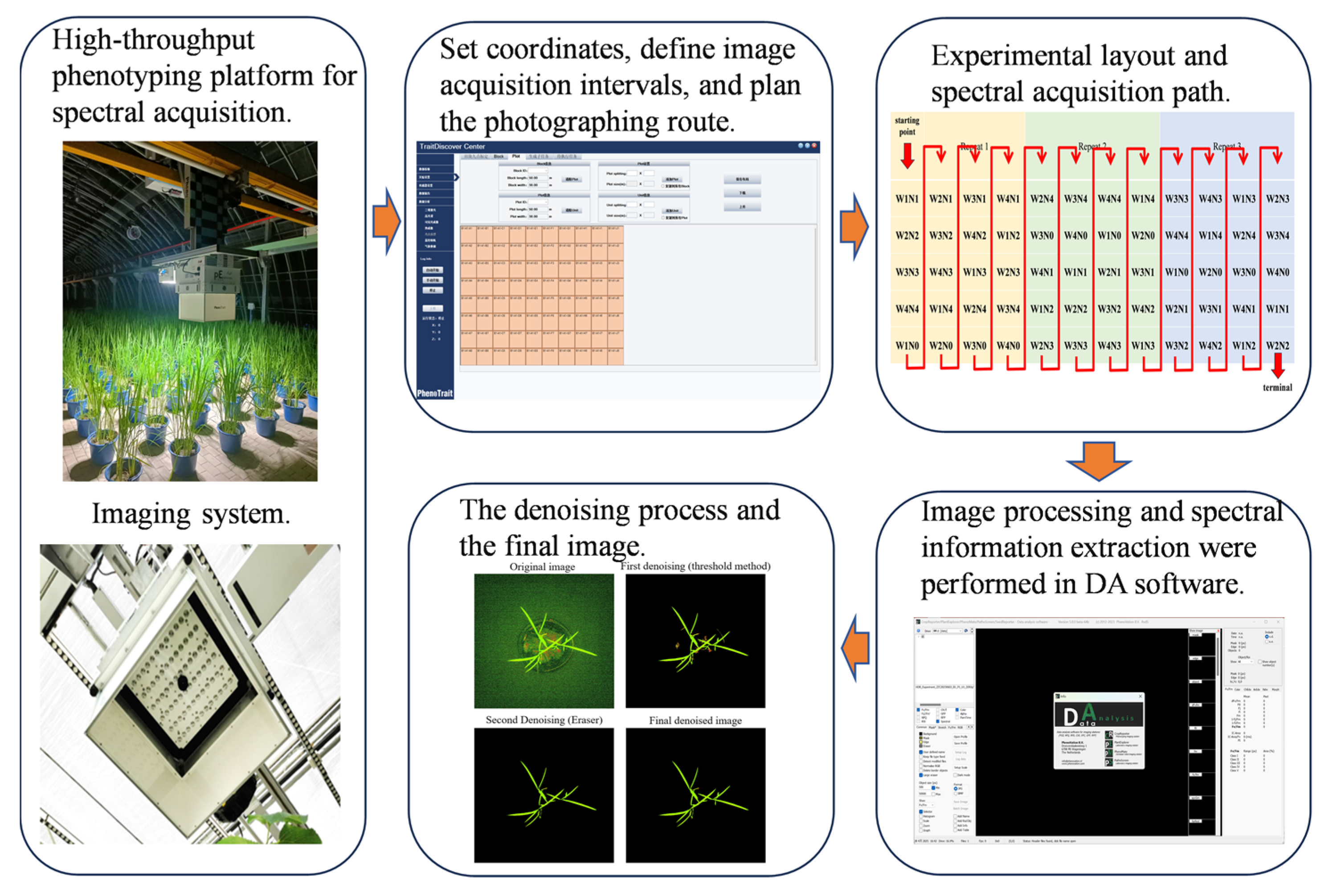
2.1. Experimental Design

The experiment was conducted from May to September 2023 at the phenotyping facility of Northeast Agricultural University, Harbin, China (126° E, 45° N). The rice cultivar used was Zhongkefa No. 5, which was transplanted on May 20. The experiment was conducted using a split-plot design, with five nitrogen (N) levels (N0–N4) assigned to the main plots and four water (W) levels (W1–W4) allocated to the subplots. Each treatment was replicated three times. The five nitrogen treatments were as follows: 0 kg/ha (N0), 45 kg/ha (N1), 90 kg/ha (N2), 135 kg/ha (N3), and 180 kg/ha (N4). Urea was used as the nitrogen source. Nitrogen fertilizer was weighed and applied separately to each pot according to its treatment level, following a fixed 5:3:2 application ratio across the basal, tillering, and panicle stages. This ratio was maintained consistently throughout the entire growing period to ensure uniform nutrient distribution. For each treatment, the required amount of fertilizer was accurately weighed for each pot using a precision balance and evenly applied into the soil by hand at the designated growth stages. Phosphorus fertilizer (P₂O₅) was applied at a rate of 80.5 kg/ha as a basal application, and potassium fertilizer (KCl) was applied at 144.9 kg/ha, with half applied as basal and half at the panicle stage. The four water treatments were defined based on the percentage of soil volumetric saturation: W1 (40%), W2 (60%), W3 (80%), and W4 (100%). Water control treatments were initiated after maximum tillering had been reached. A total of 60 potted rice plants were used in the experiment. Each pot had a surface area of 0.09 m², with a center-to-center spacing of 0.6 m between pots. The experiment involved a total of 60 pots (5 nitrogen levels × 4 water levels × 3 replicates). Each pot represented a unique treatment combination and was treated as an independent sample throughout the measurement process.

2.2. Spectral Data Acquisition and Preprocessing

Multispectral (MS), visible-light (RGB), and chlorophyll fluorescence (ChlF) data were obtained using a rail-based high-throughput phenotyping platform (HTTP) installed in the greenhouse phenotyping platform at Northeast Agricultural University (TraitDiscover, PhenoTrait, Beijing, China). The platform was equipped with multispectral, fluorescence, and RGB imaging modules, enabling the visualization of various physiological traits based on specific absorption, reflectance, and emission characteristics. The imaging system used a CCD camera with a resolution of 1.3 megapixels (1296 × 966 pixels) and a spectral sensitivity range of 400–1000 nm, ensuring sufficient spatial and spectral resolution for canopy-level measurements. Spectral data acquisition was conducted under controlled nighttime conditions using adjustable-intensity LED illumination (up to 3000 μmol·m⁻²·s⁻¹), which provided stable and uniform lighting across the imaging area. Spectral data collection was conducted at four critical growth stages of rice: tillering (TI), jointing–heading (JH), grain filling (GF), and maturity (MT). A dataset representing the full growth period (GP) was constructed by integrating data from the four individual stages to support comprehensive modeling analysis.

Image preprocessing was performed using the Data Analysis (DA; Version 5.8.0 beta-64b, PhenoVation B.V., Wageningen, The Netherlands) software provided with the TraitDiscover system. Spectral images were first imported into the DA software. Background noise from the pots and surrounding non-canopy areas was removed using a threshold-based method, which was then refined by manual cleaning with the eraser tool to eliminate residual artifacts. This preprocessing procedure was consistently applied across all sensor types to ensure that the extracted features exclusively represented the canopy region. Spectral information was then extracted using the Setup Log function. Selected spectral features were exported in text format, and the processed images were saved using the Save Image function. The overall workflow for spectral acquisition and preprocessing is illustrated in Figure 1.

2.3. Chlorophyll Index Measurement

Before each spectral data acquisition session, the relative chlorophyll index (CHI) was measured with a SPAD-502 chlorophyll meter (Konica Minolta, Tokyo, Japan). SPAD-502 measurements were used to represent CHI in this study. The device was calibrated before each measurement session using the manufacturer’s standard white calibration plate to ensure consistency and reliability. The device estimated chlorophyll concentration indirectly by comparing the absorbance of red and near-infrared light through the leaf. For each treatment, three functional leaves from the upper canopy were selected. Each leaf was measured three times at different positions (base, middle, and top), and the average of the three readings was recorded as the SPAD value for that leaf. The mean SPAD value of the top three leaves was then calculated and used as the observed canopy CHI for that treatment, aligning with the spatial scale of spectral data acquisition.

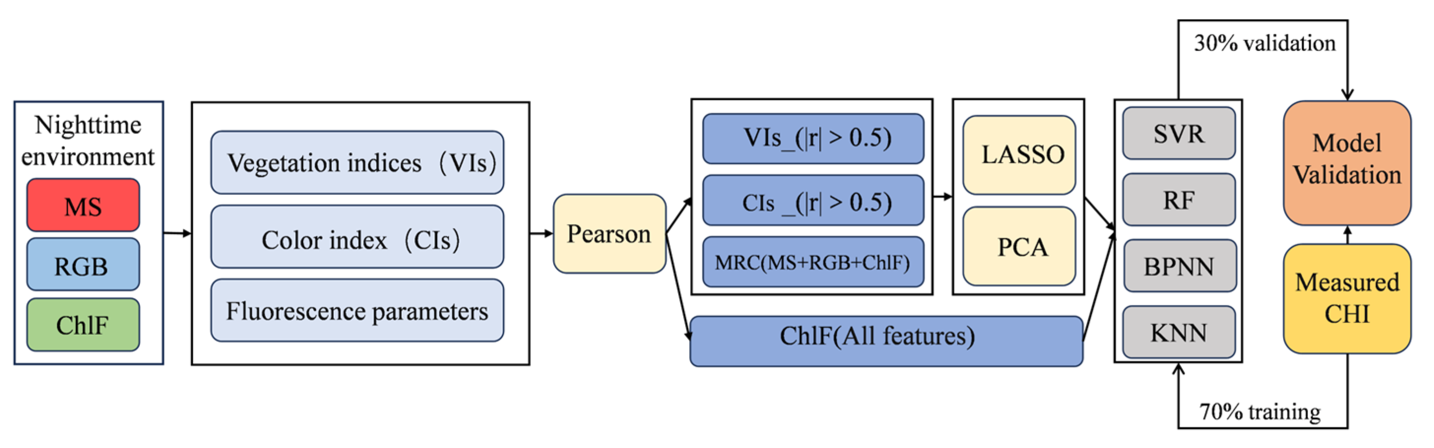
2.4. Spectral Index Selection

In this study, a total of twenty-one multispectral vegetation indices (VIs), sixteen visible-light color indices (CIs), and five chlorophyll fluorescence parameters were selected as input features. A broad set of vegetation indices was included due to the exploratory nature of nighttime spectral sensing for CHI prediction, where the optimal indices remained uncertain. The multispectral indices were calculated using the average reflectance values of the NIR, R, and G spectral bands. The color indices were computed based on combinations of the normalized r, g, and b values, with the formulas provided in the Supplementary Materials. The five chlorophyll fluorescence parameters included initial fluorescence (Fo), the efficiency of secondary electron transport in PSII (Fi), maximum fluorescence (Fm), the quantum yield of electron transport to photosystem I acceptors (1-Fi/Fm), and the maximum quantum yield of PSII photochemistry (Fv/Fm). The complete list of indices, including their names, formulas, and references, is presented in Supplementary Table S1, and the corresponding bibliographic sources are provided in the References Section [22,23,24,25,26,27,28,29,30,31,32,33,34,35,36,37,38,39,40,41,42,43,44,45,46,47,48]. The average reflectance values of the NIR, R, G, and B bands, as well as the five chlorophyll fluorescence parameters, were extracted using the Data Analysis (DA) software.

2.5. Modeling and Accuracy Evaluation

2.5.1. Machine Learning Models

The overall research framework of this study is illustrated in Figure 2. Four machine learning algorithms were employed to construct prediction models for the chlorophyll index (CHI): support vector regression (SVR), random forest regression (RF), back-propagation neural network (BPNN), and k-nearest neighbors regression (KNN).

SVR models nonlinear relationships by mapping inputs into high-dimensional spaces and seeks a regression function that fits the data with minimal error. SVR is suitable for small to medium-sized datasets and can effectively model nonlinear relationships while maintaining good generalization [49].

RF is an ensemble learning method that integrates multiple decision trees. Each tree is trained on a random subset of the data and features, and predictions are made by averaging the outputs of all trees. This structure helps RF capture variable interactions and nonlinearities effectively, while reducing the risk of overfitting and improving model stability, especially in the presence of redundant features [50].

BPNN represents a class of feedforward neural networks trained using error back-propagation. Through iterative weight adjustments via gradient descent, BPNNs are capable of learning complex nonlinear mappings between input features and target outputs. Their flexible structure makes it easier to adapt to complex variations in canopy reflectance and physiological traits [51].

KNN is a non-parametric method that estimates target values based on the average of the nearest neighbors in feature space. Although relatively simple, KNN performs well when relationships are locally linear and feature dimensionality is moderate. The simplicity of the model facilitates practical application and comparison [52]. Specifically, SVR modeling was implemented using the e1071 package, RF using random forest, BPNN with the neuralnet package, and KNN via the FNN package. All statistical analyses, model development, and figure generation were conducted in R (version 4.4.3).

2.5.2. Model Performance Evaluation

The dataset was randomly split into training and testing subsets at a ratio of 7:3. Model performance was evaluated using two standard metrics: the coefficient of determination (R²) and root mean square error (RMSE). The calculation formulas for R² and RMSE are shown in Equations (1) and (2):

$$R^2=1-{\displaystyle \frac{{\displaystyle \sum _{i=1}^n{(y_i-{\widehat{y}}_i)}^2}}{{\displaystyle \sum _{i=1}^n{(y_i-\overline{y})}^2}}}$$

(1)

$$RMSE=\sqrt{{\displaystyle \frac{1}{n}}{\displaystyle \sum _{i=1}^n{(y_i-{\widehat{y}}_i)}^2}}$$

(2)

Here, y_i represents the measured value, ŷ_i is the predicted value, ȳ is the mean of the measured values, and n denotes the sample size. A higher R² value and a lower RMSE indicate better predictive performance of the regression model.

2.6. Feature Selection Methods

Spectral features often exhibit strong multicollinearity and high dimensionality, which may interfere with model performance [53]. To reduce feature redundancy and enhance model robustness and simplicity, this study employed two variable selection methods: principal component analysis (PCA) and least absolute shrinkage and selection operator (LASSO) regression.

PCA is a commonly used dimensionality reduction technique [54] that transforms a set of correlated original variables into a new set of uncorrelated principal components (PCs), which retain the most relevant information from the original data. In this study, the principal components explaining 99% of the cumulative variance were selected for model input, ensuring that most of the data variability was preserved while minimizing interference from redundant features.

LASSO is a linear regression-based variable selection method that introduces an L₁ regularization term to shrink the coefficients of less important variables toward zero, effectively performing feature selection [55]. This method reduces model complexity and improves stability and generalization performance. Prior to modeling, all input variables were standardized. The optimal regularization parameter (λ) was determined through 10-fold cross-validation. Only features with standardized regression coefficients greater than 0.05 in absolute value were retained as relatively important variables for visualization and subsequent modeling.

3. Results

3.1. Descriptive Statistics

Significant variation in CHI was observed across the different growth stages, as shown in

Table 1. Descriptive statistics of CHI across different rice growth stages.

Period	Max	Min	Mean	SD	n	CV
TI	55.52	39.3	46.77	4.18	80	8.93
JH	55.52	41.21	49.03	3.18	80	6.48
GF	53.34	37.24	46.9	3.66	80	7.79
MT	50.93	16.61	34.76	8.42	80	24.23

Note: Summary statistics of canopy chlorophyll index (CHI) at different rice growth stages. “Max”, “Min”, “Mean”, and “SD” represent the maximum, minimum, mean, and standard deviation of CHI, respectively. “n” indicates the number of samples (n = 80 per stage). “CV” is the coefficient of variation (%), reflecting the relative dispersion of CHI values within each stage. Stages include tillering (TI), jointing–heading (JH), grain filling (GF), and maturity (MT).

and Figure 3. During the first three stages—TI, JH, and GF—CHI values remained relatively high. The JH stage exhibited the highest average CHI (49.03), while TI and GF showed comparable means of 46.77 and 46.90, respectively. The coefficients of variation (CVs) for these stages were 8.93%, 6.48%, and 7.79%, indicating relatively stable CHI within each stage. At the MT stage, CHI decreased substantially, with the mean dropping to 34.76. The minimum value declined to 16.61, and the standard deviation increased to 8.42. The CV rose to 24.23%, the highest among all stages, reflecting increased variability among individual plants. These observations are consistent with the distribution patterns shown in the violin plots. From TI to GF, the distributions were generally symmetrical and peaked, with narrow kernel curves, suggesting limited variation among individuals. In contrast, the MT stage showed a more dispersed, long-tailed distribution, indicating a higher degree of individual difference. These stage-specific differences in CHI highlight the need for modeling approaches tailored to each growth period to more accurately capture the temporal dynamics.

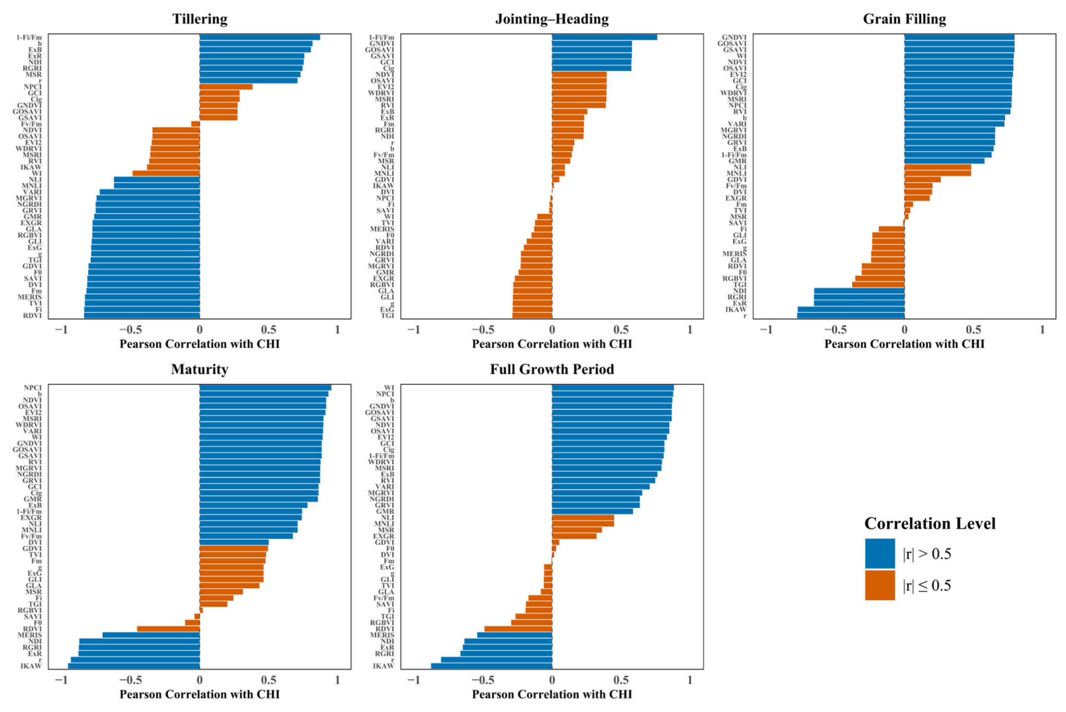
3.2. Correlation Analysis Between Spectral Features and CHI

Pearson correlation analysis was first conducted between spectral features and CHI at each growth stage. As shown in Figure 4, variables with moderate or stronger correlations (|r| > 0.5), represented by blue bars, were retained as candidate features. PCA and LASSO regression were subsequently applied to refine the feature subset and enhance model performance. Most of the selected spectral indices during the TI, GF, MT, and GP stages exhibited strong correlations with CHI, with |r| values generally above 0.5, providing a solid foundation for modeling. In contrast, during the JH stage, the correlation between CIs and CHI was relatively weak. Applying a conventional correlation threshold (|r| > 0.5) at this stage would have led to a substantial reduction in the number of available features, potentially compromising the stability and generalizability of the subsequent models. Moreover, although several ChlF features showed low correlation with CHI at certain stages, the total number of ChlF variables was limited, and their physiological relevance was well recognized. Therefore, no features from the JH-stage CIs or ChlF sensors were excluded during the correlation filtering step. All ChlF features and JH-stage CIs were retained for downstream modeling.

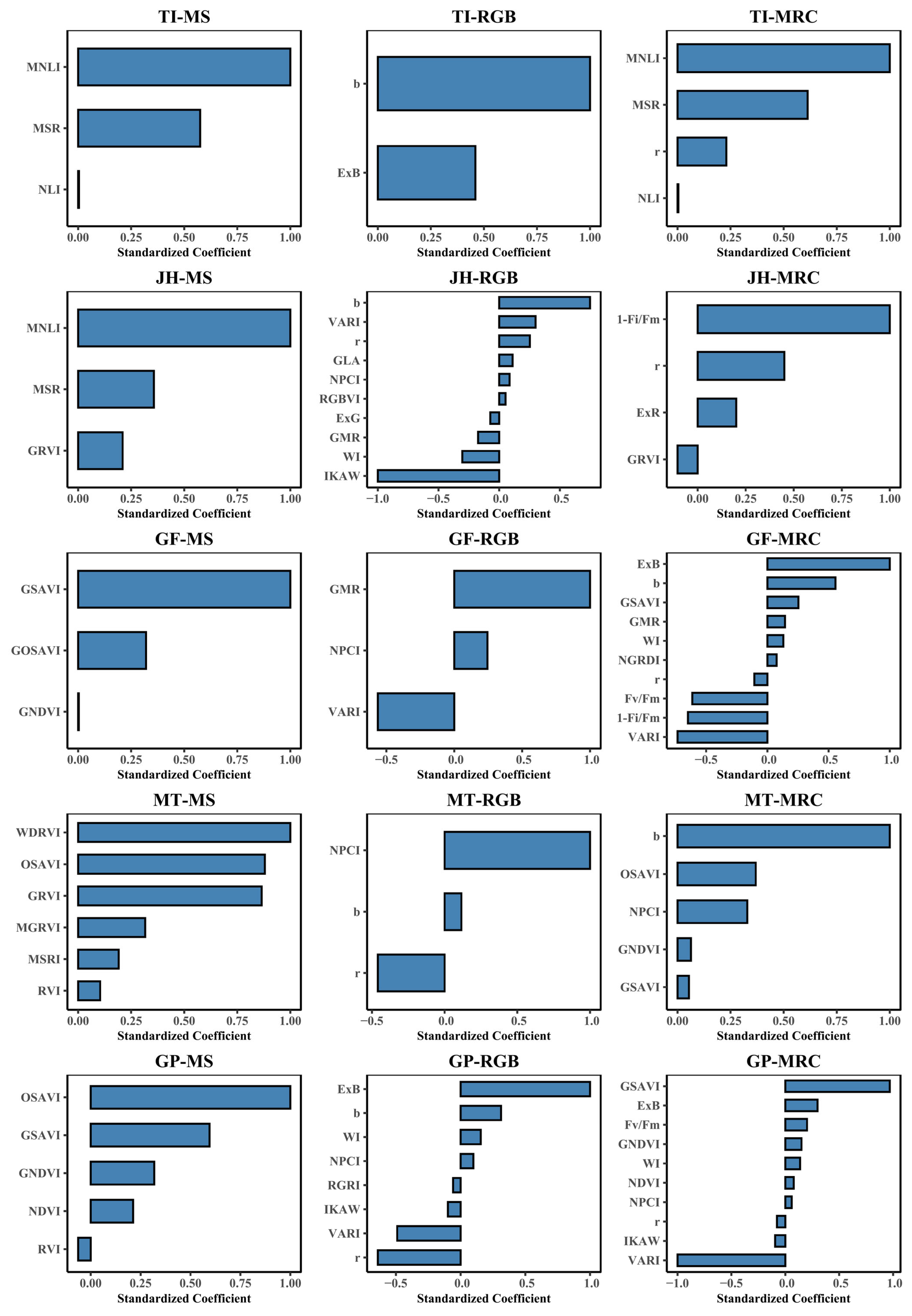
3.3. Feature Selection

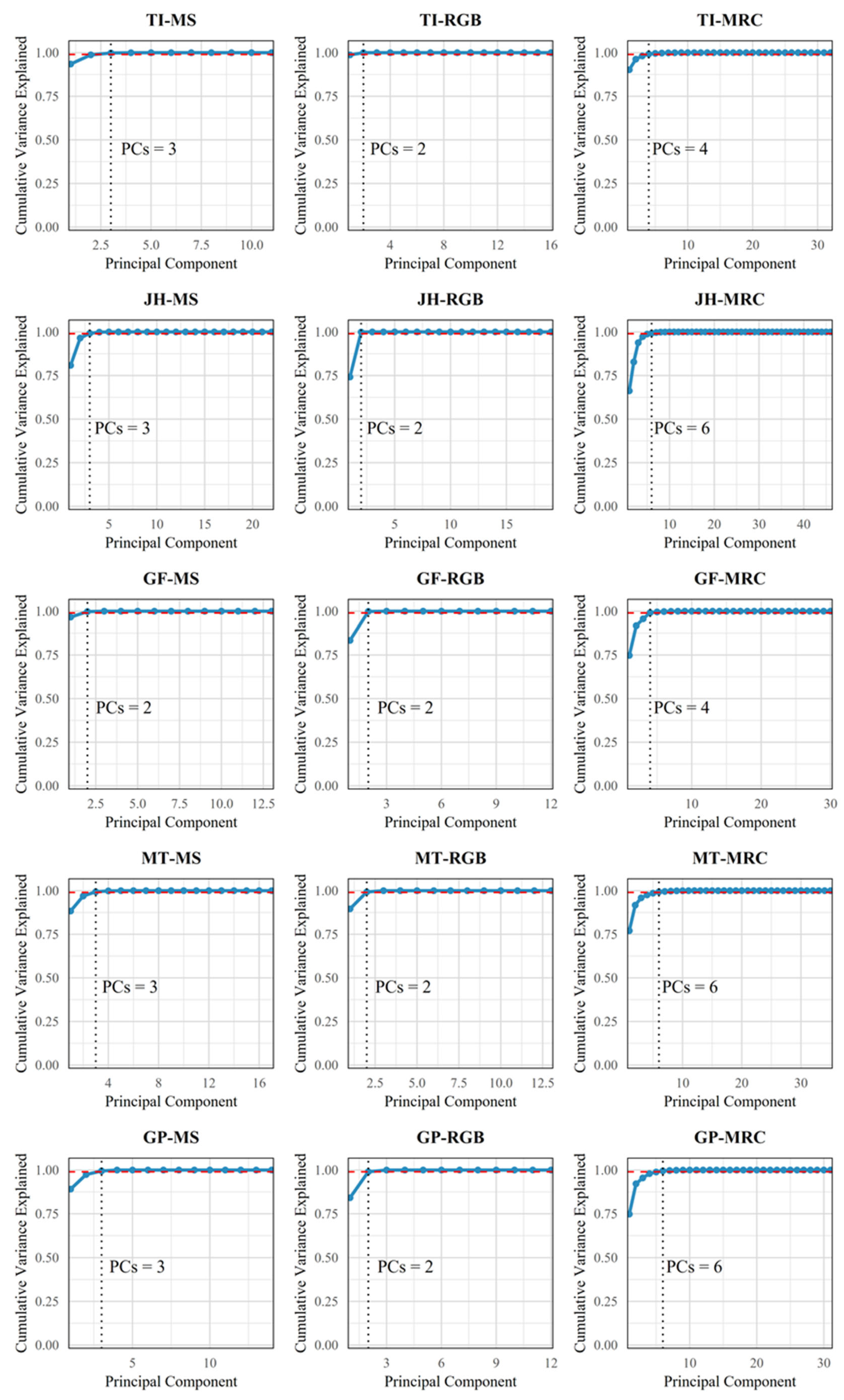
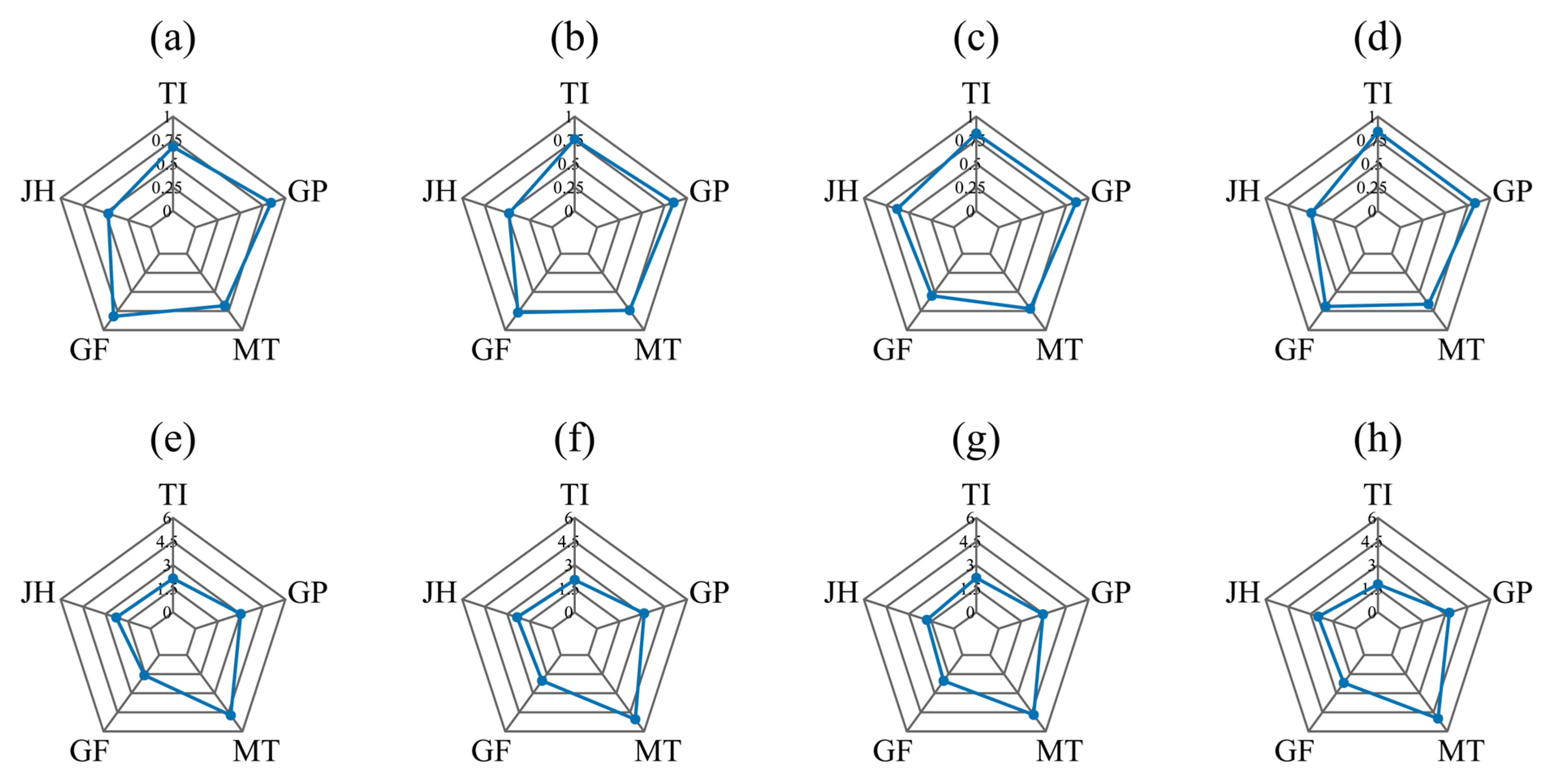
3.3.1. PCA Feature Selection Results

To evaluate the structural characteristics of variables across different growth stages and sensor combinations, PCA was performed on each dataset, and the corresponding scree plots were generated (Figure 5). As shown in Figure 5, for most datasets, the majority of information was captured within the first few principal components. The cumulative variance curves rose sharply in the early components and then quickly leveled off. Due to their relatively low dimensionality, MS and RGB datasets typically required only the first two or three principal components to explain more than 99% of the total variance. In contrast, the MRC dataset—which integrated variables from all three types of sensors—had a significantly higher initial dimensionality and required a greater number of components to reach the same variance threshold. Overall, PCA effectively extracted the major sources of variation embedded in each sensor type across different growth stages. This approach reduced redundant dimensions while preserving the core structural characteristics of the data, providing a unified, robust, and low-dimensional feature space for subsequent model construction.

3.3.2. LASSO Feature Selection Results

As shown in Figure 6, the features selected by LASSO varied considerably across different growth stages and sensor combinations. At the TI stage, the MS dataset retained MNLI, MSR, and NL1, while only two features were selected from the CI dataset. In the MRC dataset, no ChlF variables were selected, suggesting that at this stage, multispectral and RGB features alone were sufficient to explain variations in CHI, and the incremental contribution of the ChlF sensor was relatively limited. At the JH stage, MNLI and MSR were again selected from the MS dataset. Although the overall correlation between CI features and CHI was relatively low, several CI variables were still retained when all original variables were included. Interestingly, no MS features were selected in the MRC dataset at this stage, indicating that the information provided by MS might have been redundant or replaced by variables from other sensors. At the GF stage, the selected MS features differed significantly from those in earlier stages. Features from all three types of sensors were selected in the MRC dataset, and the number of retained variables increased notably, indicating that CHI prediction at this stage relied more on multi-source information. In the MT stage, the number of MS features continued to increase. The selected CI features remained similar to previous stages, while no ChlF features were retained in the MRC dataset. At the GP stage, the number of selected variables from all three types of sensors increased in the MRC dataset, reaching the highest dimensionality across all stages. It is worth noting that in some growth stages, not all types of sensors contributed retained features in the fused dataset. This may be attributed to the limited relevance of certain sensors at specific stages or redundancy among sensor-derived variables. Under LASSO’s regularization constraint, the algorithm tends to retain features with stronger explanatory power, which may lead to the exclusion of less informative or highly collinear variables.

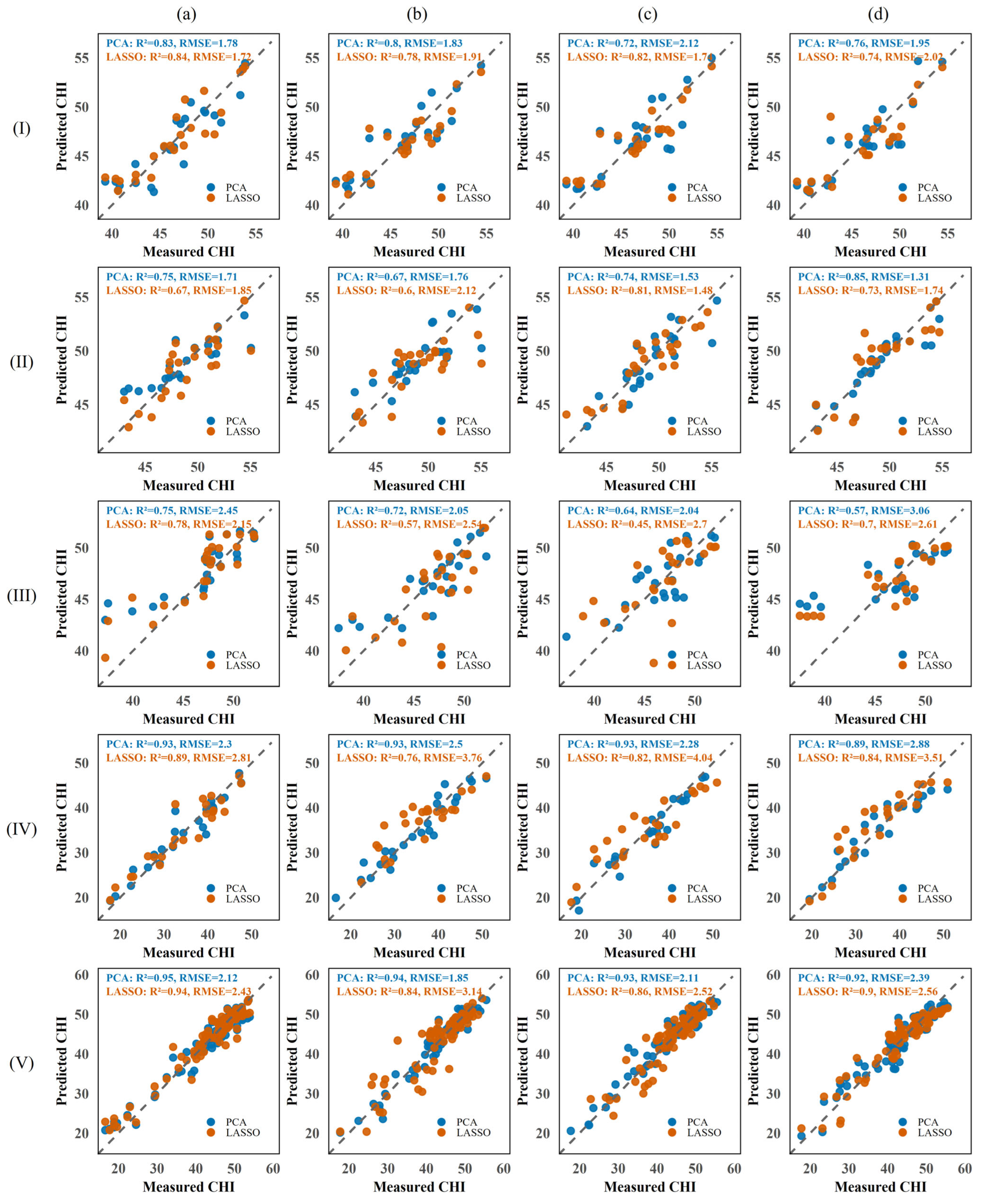
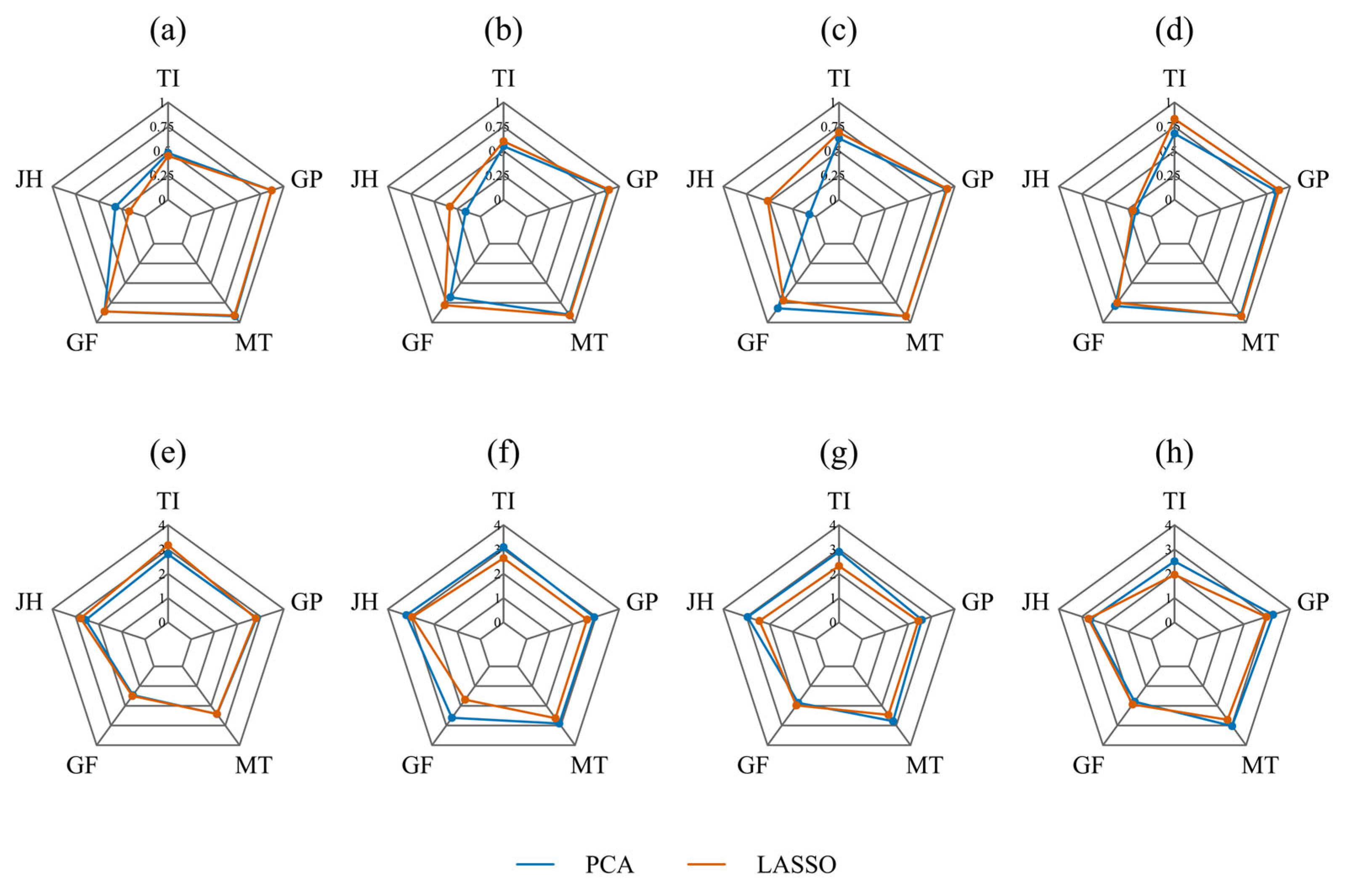
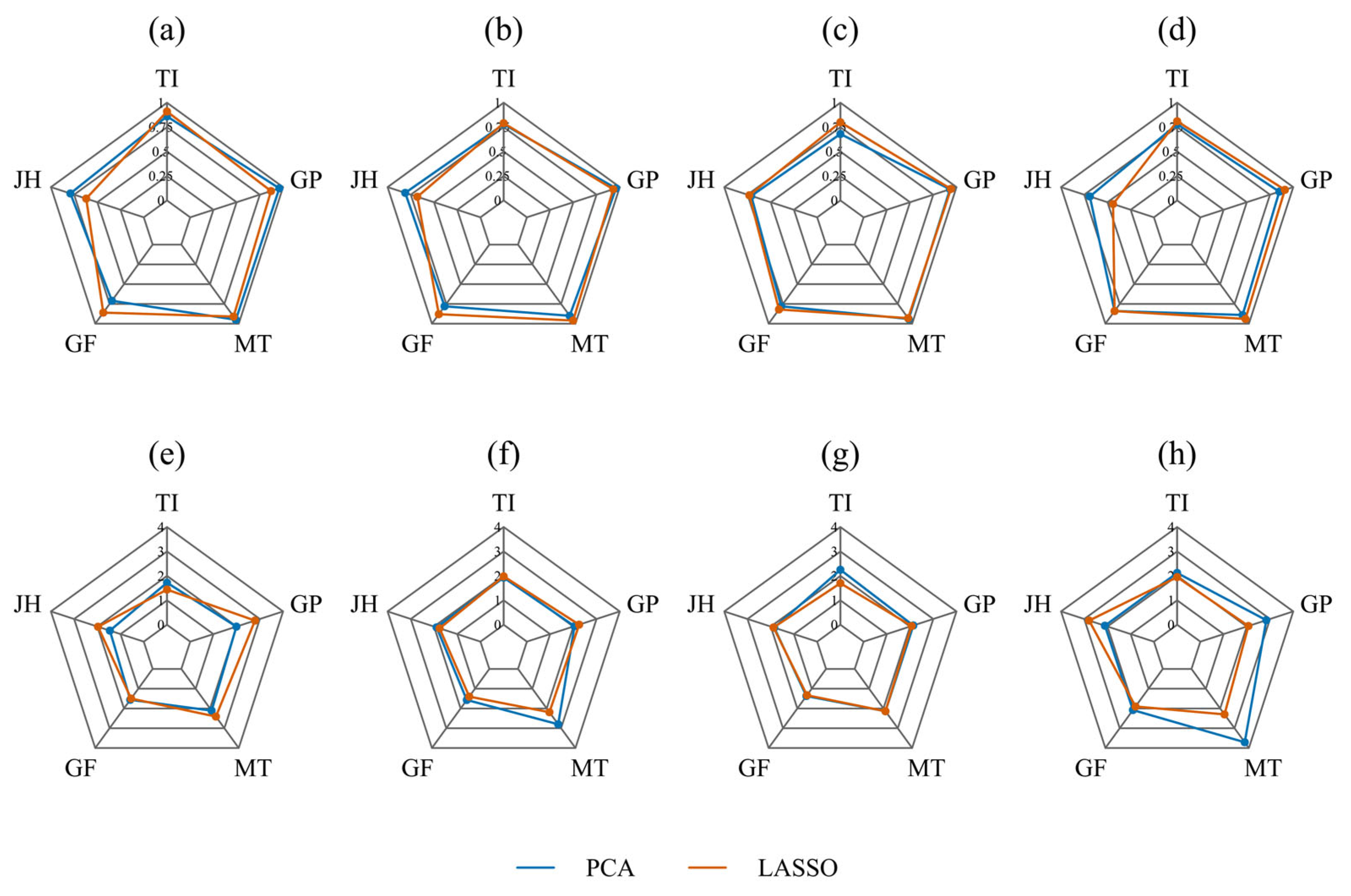
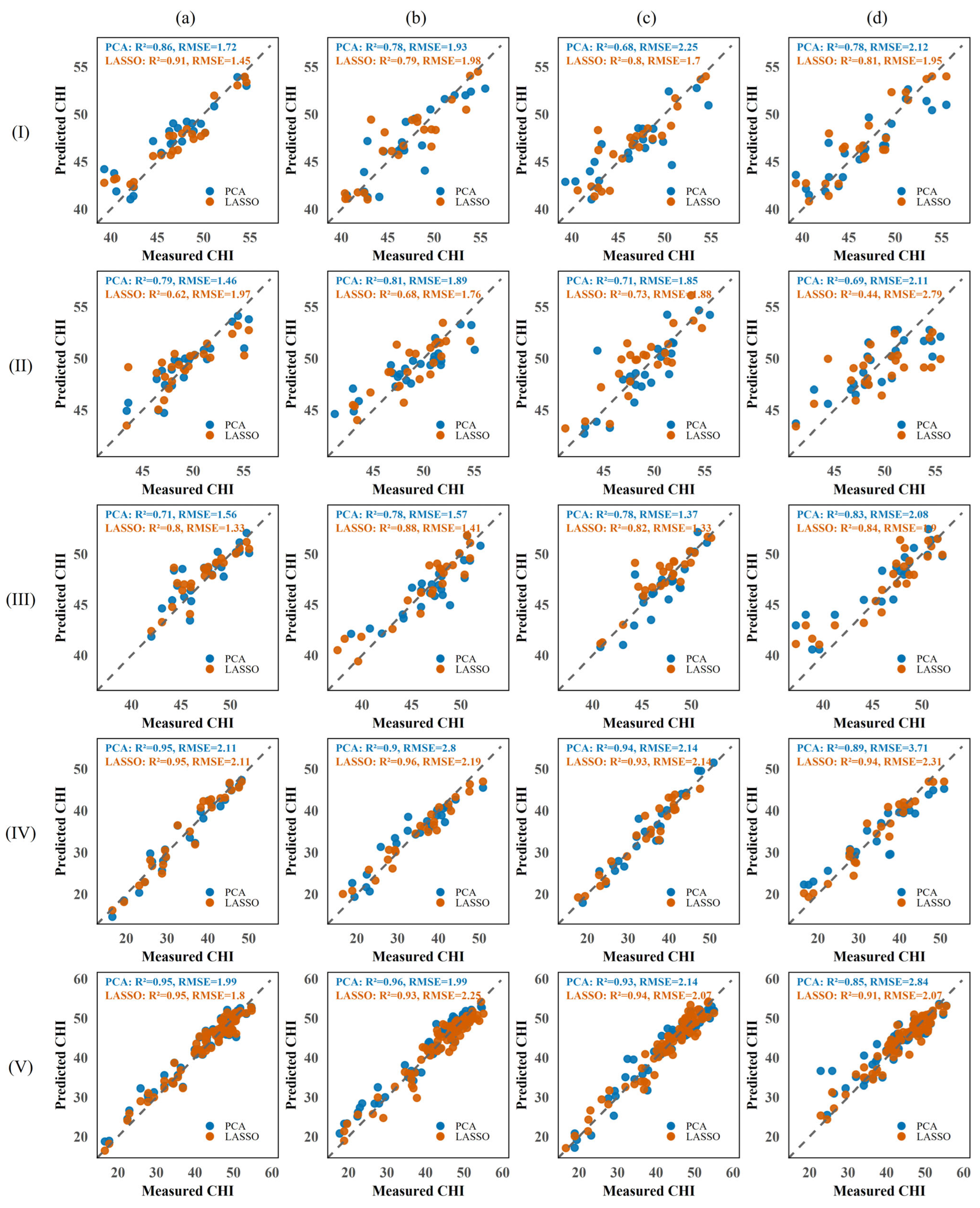
3.4. Model Performance Comparison Across Sensor Types

3.4.1. CHI Modeling Performance Using ChlF Features

The performance of models based on ChlF features on the test set is presented in Figure 7 and Figure 8. In general, the four machine learning models exhibited varying degrees of predictive accuracy across different growth stages, although the general trend was consistent. In terms of R² and RMSE values, all models achieved relatively good performance during the full GP. Notably, BPNN yielded the highest R² (0.86), followed by RF (0.85), KNN (0.83), and SVR (0.84). The corresponding RMSE values ranged from 2.95 to 3.27, indicating relatively concentrated and stable performance. In contrast, greater variability was observed in the JH and MT stages. Model errors were particularly high during the MT stage, where RF and KNN exhibited the largest RMSE values, reaching 5.05 and 4.99, respectively—the highest across all stages. Combined with the earlier descriptive statistics, the coefficient of variation in CHI values was relatively higher during the MT stage. Such variability may have introduced additional uncertainty into the modeling process, reducing the predictive reliability of ChlF features in this stage and reflecting a less stable relationship between ChlF parameters and the CHI. These results suggest that models based on chlorophyll fluorescence features showed distinct stage-dependent performance, with modeling accuracy being notably influenced by growth stage. Among the four algorithms, KNN and BPNN demonstrated relatively stable and superior predictive performance across multiple stages.

3.4.2. CHI Modeling Performance Using Multispectral Data

Regression models based on multispectral vegetation indices were developed for each growth stage using two feature selection methods: PCA and LASSO. The model’s performance on the test set is shown in Figure 9 and Figure 10. As presented in the table, PCA-based models generally outperformed LASSO-based models across most growth stages. For instance, under the SVR model, the PCA approach achieved R² values of 0.75, 0.93, and 0.95 at the JH, MT, and GP stages, respectively, with corresponding RMSEs of 1.71, 2.30, and 2.12. In contrast, the LASSO-based models yielded slightly lower R² values and noticeably higher RMSEs at the same stages. A similar trend was observed for the RF, BPNN, and KNN models, where PCA consistently demonstrated more stable and accurate performance across multiple stages. From a phenological perspective, multispectral features yielded the best predictive accuracy during the MT and GP stages. In contrast, model performance was relatively unstable at the GF stage, particularly under LASSO-selected features, where R² and RMSE values varied substantially among different models. Generally speaking, PCA provided more robust and informative feature representations than LASSO, contributing to improved model accuracy. Among the four algorithms, SVR and RF exhibited strong adaptability across stages, KNN showed advantages at specific stages, while BPNN was more sensitive to feature variations and showed greater performance fluctuation.

3.4.3. Performance of CHI Prediction Models Based on RGB Features

The performance of models constructed using RGB features is presented in Figure 11 and Figure 12. Taken together, the models demonstrated good predictive ability during the GF, MT, and GP stages, with the highest R² values reaching 0.86, 0.92, and 0.92, respectively. The corresponding RMSE values were 1.46, 2.42, and 2.43, indicating relatively accurate fits. In contrast, the model performance at the TI and JH stages was notably weaker, especially during the JH stage, where the R² values of the SVR and RF models often fell below 0.5, indicating poor prediction accuracy. This decline in early-stage performance may be attributed to insufficient chlorophyll accumulation and small plant size, which reduce the ability of RGB sensors to reliably capture CHI-related spectral variation. Regarding feature selection methods, the modeling performance of PCA and LASSO varied across growth stages. At the MT stage, both methods produced comparable results, with most models achieving R² values close to 0.9, suggesting that relevant feature information was concentrated and the dimensionality reduction method had minimal impact. At the GF stage, PCA slightly outperformed LASSO, achieving better model fits overall. In contrast, during the TI, JH, and GP stages, LASSO-selected features appeared to have stronger associations with CHI, resulting in improved predictive performance in some models.

3.4.4. Performance of CHI Prediction Models Based on Multi-Source Spectral Features

The performance of models constructed using multi-source spectral features is presented in Figure 13 and Figure 14. The models achieved better fits during the MT and GP stages, with several models reaching or approaching an R² of 0.95, indicating that the fused spectral features effectively captured the variation in CHI at these stages. In contrast, model performance during the TI, JH, and GF stages showed greater variability. For example, the R² of the LASSO-KNN model dropped to 0.44 in the JH stage, while PCA-BPNN decreased to 0.69, and PCA-SVR at the GF stage fell to 0.71. These results suggest that high-dimensional features in the early growth stages may interfere with model learning in certain algorithms. Regarding feature selection strategies, PCA and LASSO exhibited similar performance during the MT stage, where most models achieved high prediction accuracy. In the GF stage, LASSO outperformed PCA overall, particularly for the RF and BPNN models, where dimensionality reduction improved prediction considerably. During the TI and JH stages, LASSO also showed better performance in some models, likely because the retained features more directly reflected CHI differences. In contrast, PCA may have weakened subtle yet important spectral signals during dimensionality reduction, especially in earlier stages. In summary, full-spectrum feature fusion led to improved modeling accuracy during later growth stages, while in earlier stages, model performance was more sensitive to the choice of feature selection method and algorithm.

4. Discussion

4.1. Advantages of Nighttime Spectral Imaging for Chlorophyll Monitoring

In this study, we acquired canopy spectral data of rice under nighttime conditions and developed chlorophyll index (CHI) prediction models that achieved good predictive accuracy, with the highest R² reaching 0.96. This represents a marked improvement over previous studies (Table 2) conducted under natural light conditions, underscoring the feasibility and potential of nighttime spectral imaging for accurate chlorophyll monitoring in crops.

The improvement in prediction accuracy under nighttime conditions is largely attributable to the stable and consistent illumination during image acquisition. Unlike daytime conditions, where solar radiation, angle of incidence, and cloud cover introduce substantial variability, nighttime imaging eliminates these sources of noise [12]. With no ambient light interference, artificial light can evenly illuminate the canopy, resulting in consistent reflectance and improved modeling reliability [14]. Furthermore, the lower background radiation at night enhances the signal-to-noise ratio [56], making it easier to capture subtle physiological variations. Taken together, these advantages highlight the value of nighttime spectral acquisition in producing high-quality data and supporting robust vegetation monitoring applications.

Table 2. Performance comparison of CHI prediction models in rice.

Sensor	Data Collection Time	Modeling Methods	Model Accuracy (R2)	References
Multispectral	Daytime	BRT	0.712	[57]
Multispectral	Daytime	RF	0.79	[11]
Hyperspectral	Daytime	BP	0.6717	[58]
Hyperspectral	Daytime	PSO-ELM	0.791	[59]
Visible light	Daytime	AdaBoost	0.879	[60]
MS + RGB + ChlF	Nighttime	SVR	0.96	This study

Table 2. Performance comparison of CHI prediction models in rice.

Sensor	Data Collection Time	Modeling Methods	Model Accuracy (R2)	References
Multispectral	Daytime	BRT	0.712	[57]
Multispectral	Daytime	RF	0.79	[11]
Hyperspectral	Daytime	BP	0.6717	[58]
Hyperspectral	Daytime	PSO-ELM	0.791	[59]
Visible light	Daytime	AdaBoost	0.879	[60]
MS + RGB + ChlF	Nighttime	SVR	0.96	This study

4.2. Analysis of Factors Influencing Model Performance

The results of this study further confirmed that feature selection methods play a critical role in machine learning model construction, particularly when dealing with high-dimensional spectral data [61]. This finding is also supported by the ANOVA results presented in

Table 3. ANOVA results of R² and RMSE under different modeling factors.

Metric	Source of Variation	Sum of Squares	df	F-Value	p-Value
R2	Sensor	4.3591	3	100.39	<0.0001 **
	Model	0.0080	3	0.18	0.9068
	Feature Selection	0.2856	2	9.87	0.0001 **
	Stage	2.1867	4	37.77	<0.0001 **
RMSE	Sensor	15.1381	3	19.35	<0.0001 **
	Model	1.6007	3	2.05	0.1107
	Feature Selection	17.1034	2	32.79	<0.0001 **
	Stage	21.3650	4	20.48	<0.0001 **

Note: p < 0.01 (**), extremely significant; non-significant results are not marked.

(p < 0.0001). An appropriate feature selection approach can effectively eliminate redundant input variables, reduce model complexity, and, to some extent, enhance predictive accuracy [62]. In this study, we employed two feature selection methods—PCA and LASSO—to reduce feature dimensionality and improve modeling efficiency. Overall, PCA performed better when applied to multispectral sensor data, whereas LASSO yielded higher model accuracy under visible-light and multi-source fusion scenarios. In contrast, the choice of machine learning algorithms had a relatively limited impact on model performance. Although certain models appeared to differ in predictive accuracy, the ANOVA results indicated that these differences were not statistically significant (p = 0.9068).

Compared with feature selection methods and algorithm choice, sensor type exerted a more substantial influence on model performance. As evidenced by the ANOVA results (p < 0.0001; Table 3), differences among sensors led to statistically significant variation in model performance. This finding is consistent with previous studies [63]. When evaluating individual sensors, MS data produced consistently higher predictive accuracy than both RGB and ChlF data. In this study, MS-based vegetation indices were calculated using the R and NIR bands, two spectral regions highly responsive to changes in leaf chlorophyll concentration [64]. In contrast, models based on visible-light color indices generally yielded lower prediction accuracy. For instance, during the JH stage, the R² value dropped as low as 0.07. This suggests that RGB sensors, due to their limited spectral resolution, are less capable of capturing subtle biochemical differences in the canopy. Chlorophyll fluorescence parameters demonstrated variable performance across growth stages. Notably, ChlF-based models showed relatively stable performance in certain stages. For example, at the TI, GF, and GP stages, the best models achieved R² values of 0.82, 0.82, and 0.86 and RMSEs of 1.78, 1.59, and 2.95, suggesting that ChlF signals can effectively reflect CHI under specific conditions. Although single-sensor models showed reasonably good performance at certain stages, an increasing number of studies have explored multi-sensor data fusion to improve model reliability and accuracy [65,66]. By integrating complementary information from multiple spectral sources, data fusion enables a more comprehensive characterization of canopy physiological status and spectral features. In this study, models based on fused features achieved the best overall results. During the GP stage, the fusion model reached an R² of 0.96 and RMSE of 1.99, outperforming all single-sensor models. These findings indicate that sensor fusion offers more stable performance in CHI prediction.

The predictive performance of CHI models varied significantly across rice growth stages (Table 3; p < 0.0001). Overall, the GF and MT stages yielded better prediction results, whereas the TI and JH stages showed relatively poor model fit. Models trained on GP datasets also demonstrated stable performance across algorithms. In the early growth stages of rice (TI and JH), due to the small leaf area and incomplete development of the canopy structure, the acquired spectral signals were sparse and the information content was limited, which limited the predictive ability of the model [67]. As the crop entered the GF stage, the chlorophyll index usually reached its peak, the photosynthetic activity of the leaves increased, and the reflectance characteristics of the red-edge and near-infrared bands became more obvious, which enhanced the correlation between the spectral signal and CHI, thereby significantly improving the accuracy of the model. Although the R² value of the MT stage model remained at a high level, the large degree of variation in CHI during this period caused the RMSE to increase significantly at the same time. In contrast, the model built based on the GP-stage data showed a more robust performance. This is because the model integrated the spectral and physiological changes of multiple growth stages, thereby reducing the instability of the signal of a single growth stage [68].

4.3. Limitations and Future Directions

This study utilized a rail-based high-throughput phenotyping platform (HTPP) under greenhouse conditions to acquire canopy spectral data of rice using three types of sensors: multispectral, visible light, and chlorophyll fluorescence. Although the greenhouse environment can provide relatively stable measurement conditions and help control external interference factors, it cannot fully simulate the complexity of the actual field environment. Therefore, in actual agricultural production, the model may face the problem of insufficient generalization ability. In order to improve the robustness and practicality of the model, future research should gradually shift data collection and verification to field conditions. On the other hand, the sensor bands used in this study were relatively limited, which to a certain extent limited the mining of information related to the chlorophyll index. Hyperspectral sensors have higher spectral resolution and wider band coverage [69], and are expected to reveal more characteristic bands closely related to chlorophyll changes under active lighting conditions at night. In addition, with the rapid development of drone technology in the field of precision agriculture, its application in large-scale crop monitoring is becoming more and more extensive. Future research can further explore the feasibility of integrating active light sources (such as controllable LED arrays) into drone platforms to achieve nighttime spectral data collection in field environments, thereby providing more stable and reliable data support for large-scale crop canopy characteristic monitoring.

Moreover, machine learning models, especially nonlinear models, such as BPNN and KNN, generally have the “black box” problem [70], which makes it difficult to clearly explain how the model makes predictions based on the input features. Future research can introduce explanatory algorithms, such as SHAP, to quantify and visualize the contribution of each feature in model prediction, thereby providing a basis for model simplification and decision support.

5. Conclusions

In this study, crop canopy spectral data were collected using a high-throughput phenotyping platform under nighttime active illumination to estimate rice CHI. A comprehensive modeling analysis was conducted using MS, RGB, ChlF, and fused spectral data. By incorporating rice growth stage segmentation, the study further revealed stage-specific differences in sensor responsiveness to CHI dynamics. The results showed that compared to visible-light and chlorophyll fluorescence sensors, multispectral and multi-source fusion data yielded higher modeling accuracy. Furthermore, models constructed using data from the entire growth period exhibited greater stability and generalization capacity than those based on single-stage data. Notably, the fusion-based model developed for the full Growth Period (GP) stage achieved the best performance, with an R² of 0.96 and an RMSE of 1.99. This study was conducted under controlled greenhouse pot conditions, where environmental variability was limited. Although this setup allowed for high-precision measurements, it may not fully capture the complexities of field environments. Future research should validate the proposed models under open-field conditions to assess their generalizability and sensor robustness.

References

1. Nguyen, N. Global Climate Changes and Rice Food Security; FAO: Rome, Italy, 2002; Volume 625, pp. 24–30. [Google Scholar]
2. Brown, L.A.; Williams, O.; Dash, J. Calibration and characterisation of four chlorophyll meters and transmittance spectroscopy for non-destructive estimation of forest leaf chlorophyll concentration. Agric. For. Meteorol. 2022, 323, 109059. [Google Scholar] [CrossRef]
3. Zhang, R.; Yang, P.; Liu, S.; Wang, C.; Liu, J. Evaluation of the methods for estimating leaf chlorophyll content with SPAD chlorophyll meters. Remote Sens. 2022, 14, 5144. [Google Scholar] [CrossRef]
4. Tan, L.; Zhou, L.; Zhao, N.; He, Y.; Qiu, Z. Development of a low-cost portable device for pixel-wise leaf SPAD estimation and blade-level SPAD distribution visualization using color sensing. Comput. Electron. Agric. 2021, 190, 106487. [Google Scholar] [CrossRef]
5. Omia, E.; Bae, H.; Park, E.; Kim, M.S.; Baek, I.; Kabenge, I.; Cho, B.-K. Remote sensing in field crop monitoring: A comprehensive review of sensor systems, data analyses and recent advances. Remote Sens. 2023, 15, 354. [Google Scholar]
6. Ban, S.; Liu, W.; Tian, M.; Wang, Q.; Yuan, T.; Chang, Q.; Li, L. Rice leaf chlorophyll content estimation using UAV-based spectral images in different regions. Agronomy 2022, 12, 2832. [Google Scholar] [CrossRef]
7. Liu, T.; Xu, T.; Yu, F.; Yuan, Q.; Guo, Z.; Xu, B. A method combining ELM and PLSR (ELM-P) for estimating chlorophyll content in rice with feature bands extracted by an improved ant colony optimization algorithm. Comput. Electron. Agric. 2021, 186, 106177. [Google Scholar] [CrossRef]
8. Yu, F.; Xu, T.; Guo, Z.; Wen, D.; Wang, D.; Cao, Y. Remote sensing inversion of chlorophyll content in rice leaves in cold region based on Optimizing Red-edge Vegetation Index (ORVI). Smart Agric. 2020, 2, 77. [Google Scholar]
9. Saberioon, M.; Amin, M.; Anuar, A.; Gholizadeh, A.; Wayayok, A.; Khairunniza-Bejo, S. Assessment of rice leaf chlorophyll content using visible bands at different growth stages at both the leaf and canopy scale. Int. J. Appl. Earth Obs. Geoinf. 2014, 32, 35–45. [Google Scholar] [CrossRef]
10. Qiao, L.; Tang, W.; Gao, D.; Zhao, R.; An, L.; Li, M.; Sun, H.; Song, D. UAV-based chlorophyll content estimation by evaluating vegetation index responses under different crop coverages. Comput. Electron. Agric. 2022, 196, 106775. [Google Scholar] [CrossRef]
11. Wang, Y.; Tan, S.; Jia, X.; Qi, L.; Liu, S.; Lu, H.; Wang, C.; Liu, W.; Zhao, X.; He, L. Estimating relative chlorophyll content in rice leaves using unmanned aerial vehicle multi-spectral images and spectral–textural analysis. Agronomy 2023, 13, 1541. [Google Scholar] [CrossRef]
12. Nansen, C.; Savi, P.J.; Mantri, A. Methods to optimize optical sensing of biotic plant stress–combined effects of hyperspectral imaging at night and spatial binning. Plant Methods 2024, 20, 163. [Google Scholar] [CrossRef] [PubMed]
13. Xu, B.; Zhang, J.; Tang, Z.; Zhang, Y.; Xu, L.; Lu, H.; Han, Z.; Hu, W. Nighttime environment enables robust field-based high-throughput plant phenotyping: A system platform and a case study on rice. Comput. Electron. Agric. 2025, 235, 110337. [Google Scholar] [CrossRef]
14. Nguyen, H.D.D.; Pan, V.; Pham, C.; Valdez, R.; Doan, K.; Nansen, C. Night-based hyperspectral imaging to study association of horticultural crop leaf reflectance and nutrient status. Comput. Electron. Agric. 2020, 173, 105458. [Google Scholar] [CrossRef]
15. Xiang, R. Image segmentation for whole tomato plant recognition at night. Comput. Electron. Agric. 2018, 154, 434–442. [Google Scholar] [CrossRef]
16. Zhuang, J.; Wang, Q. Estimating Leaf Chlorophyll Fluorescence Parameters Using Partial Least Squares Regression with Fractional-Order Derivative Spectra and Effective Feature Selection. Remote Sens. 2025, 17, 833. [Google Scholar] [CrossRef]
17. Zheng, W.; Lu, X.; Li, Y.; Li, S.; Zhang, Y. Hyperspectral identification of chlorophyll fluorescence parameters of suaeda salsa in coastal wetlands. Remote Sens. 2021, 13, 2066. [Google Scholar] [CrossRef]
18. Porcar-Castell, A.; Tyystjärvi, E.; Atherton, J.; Van der Tol, C.; Flexas, J.; Pfündel, E.E.; Moreno, J.; Frankenberg, C.; Berry, J.A. Linking chlorophyll a fluorescence to photosynthesis for remote sensing applications: Mechanisms and challenges. J. Exp. Bot. 2014, 65, 4065–4095. [Google Scholar] [CrossRef] [PubMed]
19. Deng, Y.; Xin, N.; Zhao, L.; Shi, H.; Deng, L.; Han, Z.; Wu, G. Precision Detection of Salt Stress in Soybean Seedlings Based on Deep Learning and Chlorophyll Fluorescence Imaging. Plants 2024, 13, 2089. [Google Scholar] [CrossRef]
20. Lee, H.; Park, Y.; Kim, G.; Lee, J.H. Pre-symptomatic diagnosis of rice blast and brown spot diseases using chlorophyll fluorescence imaging. Plant Phenomics 2025, 7, 100012. [Google Scholar] [CrossRef]
21. Li, L.; Huang, G.; Wu, J.; Yu, Y.; Zhang, G.; Su, Y.; Wang, X.; Chen, H.; Wang, Y.; Wu, D. Combine photosynthetic characteristics and leaf hyperspectral reflectance for early detection of water stress. Front. Plant Sci. 2025, 16, 1520304. [Google Scholar] [CrossRef]
22. Chen, J.M.; Cihlar, J. Retrieving leaf area index of boreal conifer forests using Landsat TM images. Remote Sens. Environ. 1996, 55, 153–162. [Google Scholar] [CrossRef]
23. Bagheri, N. Application of aerial remote sensing technology for detection of fire blight infected pear trees. Comput. Electron. Agric. 2020, 168, 105147. [Google Scholar] [CrossRef]
24. Haboudane, D.; Miller, J.R.; Tremblay, N.; Zarco-Tejada, P.J.; Dextraze, L. Integrated narrow-band vegetation indices for prediction of crop chlorophyll content for application to precision agriculture. Remote Sens. Environ. 2002, 81, 416–426. [Google Scholar] [CrossRef]
25. Jiang, Z.; Huete, A.R.; Didan, K.; Miura, T. Development of a two-band enhanced vegetation index without a blue band. Remote Sens. Environ. 2008, 112, 3833–3845. [Google Scholar] [CrossRef]
26. Raper, T.; Varco, J. Canopy-scale wavelength and vegetative index sensitivities to cotton growth parameters and nitrogen status. Precis. Agric. 2015, 16, 62–76. [Google Scholar] [CrossRef]
27. Rondeaux, G.; Steven, M.; Baret, F. Optimization of soil-adjusted vegetation indices. Remote Sens. Environ. 1996, 55, 95–107. [Google Scholar] [CrossRef]
28. Huete, A.R. A soil-adjusted vegetation index (SAVI). Remote Sens. Environ. 1988, 25, 295–309. [Google Scholar] [CrossRef]
29. Gong, P.; Pu, R.; Biging, G.S.; Larrieu, M.R. Estimation of forest leaf area index using vegetation indices derived from Hyperion hyperspectral data. IEEE Trans. Geosci. Remote Sens. 2003, 41, 1355–1362. [Google Scholar] [CrossRef]
30. Feng, W.; Wu, Y.; He, L.; Ren, X.; Wang, Y.; Hou, G.; Wang, Y.; Liu, W.; Guo, T. An optimized non-linear vegetation index for estimating leaf area index in winter wheat. Precis. Agric. 2019, 20, 1157–1176. [Google Scholar] [CrossRef]
31. Goel, N.S.; Qin, W. Influences of canopy architecture on relationships between various vegetation indices and LAI and FPAR: A computer simulation. Remote Sens. Rev. 1994, 10, 309–347. [Google Scholar] [CrossRef]
32. Poley, L.G.; McDermid, G.J. A systematic review of the factors influencing the estimation of vegetation aboveground biomass using unmanned aerial systems. Remote Sens. 2020, 12, 1052. [Google Scholar] [CrossRef]
33. Xu, T.; Wang, F.; Shi, Z.; Miao, Y. Multi-scale monitoring of rice aboveground biomass by combining spectral and textural information from UAV hyperspectral images. Int. J. Appl. Earth Obs. Geoinf. 2024, 127, 103655. [Google Scholar] [CrossRef]
34. Sankaran, S.; Zhou, J.; Khot, L.R.; Trapp, J.J.; Mndolwa, E.; Miklas, P.N. High-throughput field phenotyping in dry bean using small unmanned aerial vehicle based multispectral imagery. Comput. Electron. Agric. 2018, 151, 84–92. [Google Scholar] [CrossRef]
35. Roujean, J.-L.; Breon, F.-M. Estimating PAR absorbed by vegetation from bidirectional reflectance measurements. Remote Sens. Environ. 1995, 51, 375–384. [Google Scholar] [CrossRef]
36. Wilson, R.J.; Haas, R.; Schelland, J.; Deering, D. Monitoring vegetation systems in the Great Plains with ERTS. NASA Spec. Publ 1974, 351, 309R. [Google Scholar]
37. Bendig, J.; Yu, K.; Aasen, H.; Bolten, A.; Bennertz, S.; Broscheit, J.; Gnyp, M.L.; Bareth, G. Combining UAV-based plant height from crop surface models, visible, and near infrared vegetation indices for biomass monitoring in barley. Int. J. Appl. Earth Obs. Geoinf. 2015, 39, 79–87. [Google Scholar] [CrossRef]
38. Sripada, R.P.; Heiniger, R.W.; White, J.G.; Weisz, R. Aerial color infrared photography for determining late-season nitrogen requirements in corn. Agron. J. 2005, 97, 1443–1451. [Google Scholar] [CrossRef]
39. Putra, A.N.; Kristiawati, W.; Mumtazydah, D.C.; Anggarwati, T.; Annisa, R.; Sholikah, D.H.; Okiyanto, D. Pineapple biomass estimation using unmanned aerial vehicle in various forcing stage: Vegetation index approach from ultra-high-resolution image. Smart Agric. Technol. 2021, 1, 100025. [Google Scholar] [CrossRef]
40. Gitelson, A.A.; Gritz, Y.; Merzlyak, M.N. Relationships between leaf chlorophyll content and spectral reflectance and algorithms for non-destructive chlorophyll assessment in higher plant leaves. J. Plant Physiol. 2003, 160, 271–282. [Google Scholar] [CrossRef]
41. Zhang, Y.; Jiang, Y.; Xu, B.; Yang, G.; Feng, H.; Yang, X.; Yang, H.; Liu, C.; Cheng, Z.; Feng, Z. Study on the Estimation of Leaf Area Index in Rice Based on UAV RGB and Multispectral Data. Remote Sens. 2024, 16, 3049. [Google Scholar] [CrossRef]
42. El Hafyani, M.; Saddik, A.; Hssaisoune, M.; Labbaci, A.; Tairi, A.; Abdelfadel, F.; Bouchaou, L. Weeds detection in a citrus orchard using multispectral UAV data and machine learning algorithms: A Case Study from Souss-Massa basin, Morocco. Remote Sens. Appl. Soc. Environ. 2025, 38, 101553. [Google Scholar] [CrossRef]
43. Gerardo, R.; de Lima, I.P. Applying RGB-based vegetation indices obtained from UAS imagery for monitoring the rice crop at the field scale: A case study in Portugal. Agriculture 2023, 13, 1916. [Google Scholar] [CrossRef]
44. Li, J.; Wang, W.; Sheng, Y.; Anwar, S.; Su, X.; Nian, Y.; Yue, H.; Ma, Q.; Liu, J.; Li, X. Rice Yield Estimation Based on Cumulative Time Series Vegetation Indices of UAV MS and RGB Images. Agronomy 2024, 14, 2956. [Google Scholar] [CrossRef]
45. Woebbecke, D.M.; Meyer, G.E.; Von Bargen, K.; Mortensen, D.A. Color indices for weed identification under various soil, residue, and lighting conditions. Trans. ASAE 1995, 38, 259–269. [Google Scholar] [CrossRef]
46. Li, Z.; Feng, X.; Li, J.; Wang, D.; Hong, W.; Qin, J.; Wang, A.; Ma, H.; Yao, Q.; Chen, S. Time Series Field Estimation of Rice Canopy Height Using an Unmanned Aerial Vehicle-Based RGB/Multispectral Platform. Agronomy 2024, 14, 883. [Google Scholar] [CrossRef]
47. Roháček, K. Chlorophyll fluorescence parameters: The definitions, photosynthetic meaning, and mutual relationships. Photosynthetica 2002, 40, 13–29. [Google Scholar] [CrossRef]
48. Xia, Q.; Tan, J.; Cheng, S.; Jiang, Y.; Guo, Y. Sensing plant physiology and environmental stress by automatically tracking Fj and Fi features in PSII chlorophyll fluorescence induction. Photochem. Photobiol. 2019, 95, 1495–1503. [Google Scholar] [CrossRef]
49. Awad, M.; Khanna, R.; Awad, M.; Khanna, R. Support vector regression. In Efficient Learning Machines: Theories, Concepts, and Applications for Engineers and System Designers; Apress: Berlin/Heidelberg, Germany, 2015; pp. 67–80. [Google Scholar]
50. Breiman, L. Random forests. Mach. Learn. 2001, 45, 5–32. [Google Scholar] [CrossRef]
51. Song, E.; Shao, G.; Zhu, X.; Zhang, W.; Dai, Y.; Lu, J. Estimation of plant height and biomass of rice using unmanned aerial vehicle. Agronomy 2024, 14, 145. [Google Scholar] [CrossRef]
52. Hemalatha, N.; Akhil, W.; Vinod, R. Computational yield prediction of Rice using KNN regression. In Computer Vision and Robotics: Proceedings of CVR 2022; Springer: Berlin/Heidelberg, Germany, 2023; pp. 295–308. [Google Scholar]
53. Yang, M.-D.; Hsu, Y.-C.; Tseng, W.-C.; Tseng, H.-H.; Lai, M.-H. Precision assessment of rice grain moisture content using UAV multispectral imagery and machine learning. Comput. Electron. Agric. 2025, 230, 109813. [Google Scholar] [CrossRef]
54. Tian, L.; Li, Y.; Zhang, M. A variable selection method based on multicollinearity reduction for food origin traceability identification. Vib. Spectrosc. 2025, 138, 103804. [Google Scholar] [CrossRef]
55. Xu, S.; Xu, X.; Blacker, C.; Gaulton, R.; Zhu, Q.; Yang, M.; Yang, G.; Zhang, J.; Yang, Y.; Yang, M. Estimation of leaf nitrogen content in rice using vegetation indices and feature variable optimization with information fusion of multiple-sensor images from UAV. Remote Sens. 2023, 15, 854. [Google Scholar] [CrossRef]
56. Wong, C.Y.S.; McHugh, D.P.; Bambach, N.; McElrone, A.J.; Alsina, M.M.; Kustas, W.P.; Magney, T.S. Hyperspectral and Photodiode Retrievals of Nighttime LED-Induced Chlorophyll Fluorescence (LEDIF) for Tracking Photosynthetic Phenology in a Vineyard. J. Geophys. Res. Biogeosci. 2024, 129, e2023JG007742. [Google Scholar] [CrossRef]
57. Gu, Q.; Huang, F.; Lou, W.; Zhu, Y.; Hu, H.; Zhao, Y.; Zhou, H.; Zhang, X. Unmanned aerial vehicle-based assessment of rice leaf chlorophyll content dynamics across genotypes. Comput. Electron. Agric. 2024, 221, 108939. [Google Scholar] [CrossRef]
58. Liu, H.; Lei, X.; Liang, H.; Wang, X. Multi-Model Rice Canopy Chlorophyll Content Inversion Based on UAV Hyperspectral Images. Sustainability 2023, 15, 7038. [Google Scholar] [CrossRef]
59. Cao, Y.; Jiang, K.; Wu, J.; Yu, F.; Du, W.; Xu, T. Inversion modeling of japonica rice canopy chlorophyll content with UAV hyperspectral remote sensing. PLoS ONE 2020, 15, e0238530. [Google Scholar] [CrossRef] [PubMed]
60. Jing, H.; Bin, W.; Jiachen, H. Chlorophyll inversion in rice based on visible light images of different planting methods. PLoS ONE 2025, 20, e0319657. [Google Scholar] [CrossRef]
61. Fei, S.; Li, L.; Han, Z.; Chen, Z.; Xiao, Y. Combining novel feature selection strategy and hyperspectral vegetation indices to predict crop yield. Plant Methods 2022, 18, 119. [Google Scholar] [CrossRef]
62. Elsherbiny, O.; Fan, Y.; Zhou, L.; Qiu, Z. Fusion of Feature Selection Methods and Regression Algorithms for Predicting the Canopy Water Content of Rice Based on Hyperspectral Data. Agriculture 2021, 11, 51. [Google Scholar] [CrossRef]
63. Yuan, Y.; Wang, X.; Shi, M.; Wang, P. Performance comparison of RGB and multispectral vegetation indices based on machine learning for estimating Hopea hainanensis SPAD values under different shade conditions. Front. Plant Sci. 2022, 13, 928953. [Google Scholar] [CrossRef]
64. Lu, S.; Lu, F.; You, W.; Wang, Z.; Liu, Y.; Omasa, K. A robust vegetation index for remotely assessing chlorophyll content of dorsiventral leaves across several species in different seasons. Plant Methods 2018, 14, 15. [Google Scholar] [CrossRef] [PubMed]
65. Karmakar, P.; Teng, S.W.; Murshed, M.; Pang, S.; Li, Y.; Lin, H. Crop monitoring by multimodal remote sensing: A review. Remote Sens. Appl. Soc. Environ. 2024, 33, 101093. [Google Scholar] [CrossRef]
66. Zhu, H.; Liang, S.; Lin, C.; He, Y.; Xu, J.-L. Using Multi-Sensor Data Fusion Techniques and Machine Learning Algorithms for Improving UAV-Based Yield Prediction of Oilseed Rape. Drones 2024, 8, 642. [Google Scholar] [CrossRef]
67. Gong, Y.; Yang, K.; Lin, Z.; Fang, S.; Wu, X.; Zhu, R.; Peng, Y. Remote estimation of leaf area index (LAI) with unmanned aerial vehicle (UAV) imaging for different rice cultivars throughout the entire growing season. Plant Methods 2021, 17, 88. [Google Scholar] [CrossRef]
68. Wan, L.; Cen, H.; Zhu, J.; Zhang, J.; Zhu, Y.; Sun, D.; Du, X.; Zhai, L.; Weng, H.; Li, Y.; et al. Grain yield prediction of rice using multi-temporal UAV-based RGB and multispectral images and model transfer—a case study of small farmlands in the South of China. Agric. For. Meteorol. 2020, 291, 108096. [Google Scholar] [CrossRef]
69. Ram, B.G.; Oduor, P.; Igathinathane, C.; Howatt, K.; Sun, X. A systematic review of hyperspectral imaging in precision agriculture: Analysis of its current state and future prospects. Comput. Electron. Agric. 2024, 222, 109037. [Google Scholar] [CrossRef]
70. Araújo, S.O.; Peres, R.S.; Ramalho, J.C.; Lidon, F.; Barata, J. Machine Learning Applications in Agriculture: Current Trends, Challenges, and Future Perspectives. Agronomy 2023, 13, 2976. [Google Scholar] [CrossRef]
Figure 1. A workflow of spectral data acquisition and preprocessing.
Agriculture 15 01425 g001
Figure 2. Workflow of the study, including spectral data acquisition using multi-source sensors (MS, RGB, and ChlF), preprocessing, vegetation index calculation, model construction using four machine learning algorithms, and performance evaluation.
Agriculture 15 01425 g002
Figure 3. Violin plots of CHI across different rice growth stages. Each colored violin represents the distribution of CHI values at a specific stage: tillering (TI), jointing–heading (JH), grain filling (GF), and maturity (MT). Black dots represent individual data points, and the solid line connects the mean CHI value at each stage, illustrating the temporal trend.
Agriculture 15 01425 g003
Figure 4. Pearson correlation analysis between vegetation indices and CHI at different rice growth stages. Bars are sorted by the correlation value. Features with absolute correlation greater than 0.5 are colored in blue, while the others are shown in orange.
Agriculture 15 01425 g004
Figure 5. PCA-based feature selection. Each subplot represents a combination of rice growth stage (TI, JH, GF, MT, and GP) and sensor type (MS, RGB, and MRC). The dashed vertical line indicates the number of principal components (PCs) retained for modeling, ensuring that over 99% of the total variance is explained. The red line shows the cumulative variance explained, while the blue points and connecting line represent the variance explained by each individual principal component.
Agriculture 15 01425 g005
Figure 6. LASSO-based feature selection. Each subplot corresponds to a combination of growth stage (TI, JH, GF, MT, and GP) and sensor type (MS, RGB, and MRC). Bars indicate selected features, with length representing the magnitude and sign of their standardized coefficients in predicting the chlorophyll index (CHI).
Agriculture 15 01425 g006
Figure 7. Performance of machine learning models using chlorophyll fluorescence parameters for estimating the rice chlorophyll index at different growth stages. Subplots (ad) show the coefficient of determination (R2), and (eh) show the root mean square error (RMSE) across five rice growth stages: TI (tillering), JH (jointing–heading), GF (grain filling), MT (maturity), and GP (full growth period). Each column corresponds to a machine learning model: SVR, RF, BPNN, and KNN.
Agriculture 15 01425 g007
Figure 8. CHI prediction performance based on chlorophyll fluorescence features. Prediction accuracy of the CHI across different rice growth stages ((IV): tillering, jointing–heading, grain filling, maturity, and full growth period) and four machine learning models ((ad): SVR, RF, BPNN, and KNN). Each dot represents a field sample (n = 80 per stage). Due to overlapping phenological periods, the full growth period dataset contained 240 unique samples. Dashed lines denote 1:1 reference lines.
Agriculture 15 01425 g008
Figure 9. Radar plots comparing the model performance of PCA and LASSO feature selection across different rice growth stages based on multispectral data. PCA (blue) and LASSO (orange). Subplots (ad) show the coefficient of determination (R2), and (eh) show the root mean square error (RMSE) across five rice growth stages: TI (tillering), JH (jointing–heading), GF (grain filling), MT (maturity), and GP (full growth period). Each column corresponds to a machine learning model: SVR, RF, BPNN, and KNN.
Agriculture 15 01425 g009
Figure 10. CHI prediction performance based on multispectral features. Prediction accuracy of the CHI using PCA (blue) and LASSO (orange) feature selection across five rice growth stages ((IV): tillering, jointing–heading, grain filling, maturity, and full growth period) and four machine learning models ((ad): SVR, RF, BPNN, and KNN). Each dot represents a field sample (n = 80 per stage). Due to overlapping phenological periods, the full growth period dataset contained 240 unique samples. Dashed lines denote 1:1 reference lines.
Agriculture 15 01425 g010
Figure 11. Radar plots comparing the model performance of PCA and LASSO feature selection across different rice growth stages based on RGB data. PCA (blue) and LASSO (orange). Subplots (ad) show the coefficient of determination (R2), and (eh) show the root mean square error (RMSE) across five rice growth stages: TI (tillering), JH (jointing–heading), GF (grain filling), MT (maturity), and GP (full growth period). Each column corresponds to a machine learning model: SVR, RF, BPNN, and KNN.
Agriculture 15 01425 g011
Figure 12. CHI prediction performance based on RGB features. Prediction accuracy of the CHI using PCA (blue) and LASSO (orange) feature selection across five rice growth stages ((IV): tillering, jointing–heading, grain filling, maturity, and full growth period) and four machine learning models ((ad): SVR, RF, BPNN, and KNN). Each dot represents a field sample (n = 80 per stage). Due to overlapping phenological periods, the full growth period dataset contained 240 unique samples. Dashed lines denote 1:1 reference lines.
Agriculture 15 01425 g012
Figure 13. Radar plots comparing the model performance of PCA and LASSO feature selection across different rice growth stages based on multi-source fused data. PCA (blue) and LASSO (orange). Subplots (ad) show the coefficient of determination (R2), and (eh) show the root mean square error (RMSE) across five rice growth stages: TI (tillering), JH (jointing–heading), GF (grain filling), MT (maturity), and GP (full growth period). Each column corresponds to a machine learning model: SVR, RF, BPNN, and KNN.
Agriculture 15 01425 g013
Figure 14. CHI prediction performance based on multi-source fused spectral features. Prediction accuracy of the CHI using PCA (blue) and LASSO (orange) feature selection across five rice growth stages ((IV): tillering, jointing–heading, grain filling, maturity, and full growth period) and four machine learning models ((ad): SVR, RF, BPNN, and KNN). Each dot represents a field sample (n = 80 per stage). Due to overlapping phenological periods, the full growth period dataset contained 240 unique samples. Dashed lines denote 1:1 reference lines.
Agriculture 15 01425 g014