Article

Effect of Angle Between Center-Mounted Blades and Disc on Particle Trajectory Correction in Side-Throwing Centrifugal Spreaders

1
College of Engineering, Northeast Agricultural University, Harbin 150030, China
2
College of Mechanical and Electrical Engineering, Suqian University, Suqian 223800, China
*
Author to whom correspondence should be addressed.
Agriculture 2025, 15(13), 1392; https://doi.org/10.3390/agriculture15131392
Submission received: 22 May 2025 / Revised: 23 June 2025 / Accepted: 25 June 2025 / Published: 28 June 2025

Abstract

This study investigated the effect of the angle between the blade and the inclined disc on particle trajectory correction during ejection from an organic fertilizer side-throwing device. Using the inclined disc device as the test subject, a blade-based coordinate system was established to model the complex relative particle motion under combined disc and blade inclination. Particle dynamics and blade forces were analyzed quadrantally, enabling the development of a mechanical model and the derivation of displacement equations. Numerical simulation, virtual simulation, and experimental testing yielded the following results: Under the current device parameters, the relative velocity between particles and the blade reaches its maximum when the angle between the blade and the inclined disc is 80°. Within the angle range from 65° to 85°, as the angle increases, the scattering angle of single-sided discs monotonically decreases, while that of dual-sided discs monotonously increases. At an angle of 65°, the trajectories of the dual-sided disc flows tend to converge. At 80°, the flow is at the critical point between convergence and divergence. The effective throwing distance first increases and then decreases, reaching a maximum at an angle of 80°. This study clarifies the relationship between the angle correction of blade–disc inclination and particle velocity and trajectory on the blade, providing a reliable mathematical model and simulation method for similar studies in the field of inclined disc centrifugal material ejection.

1. Introduction

Centrifugal spreading represents a widely adopted material processing technique [1,2,3]. This technology demonstrates extensive applicability across diverse sectors, including agriculture, pharmaceuticals, food processing, material handling, and environmental management [4,5,6,7]. Organic fertilizer serves as a vital nutrient source for enhancing soil activation, aeration, and remediating soil compaction [8,9,10,11,12] and is conventionally distributed in agricultural production using centrifugal spreaders [13,14,15,16,17]. While conventional horizontal-disc spreaders produce broad distributions, side-throwing centrifugal spreaders with tilted discs generate narrow-width, long-range streams essential for complex field conditions [18,19,20]. Centered blade mounting proves advantageous due to its manufacturing simplicity, maximal material-bearing capacity, and comparability with conventional designs. Therefore, with fixed centered mounting and a constant bearing area, optimizing the blade tilt becomes a critical factor in trajectory correction to satisfy side-throwing centrifugal spreader performance specifications [21].
Establishing a mathematical model is essential to quantifying blade–particle interactions in a side-throwing centrifugal spreader. This dual-inclination system (disc tilt + blade tilt) generates complex dynamic patterns in which particle displacement and resultant forces exhibit continuous spatiotemporal variations in the base coordinate system. The current literature lacks direct references for this specific configuration. Recent advances in horizontal-disc modeling include V.B. Cerović et al., who incorporated blade tilt into mechanical equations to improve trajectory simulation accuracy [22]; T Kurt et al., who developed comprehensive models using hyperbolic cosine functions for granular motion description [23]; and A. Martínez-Rodríguez et al., who implemented computational solutions in Mathcad for automated velocity calculations [24]. Notable innovations included Zhang Guozhong’s angled-blade design revealing axial acceleration interdependencies [25] and Liu Cailing’s guide rail system demonstrating force-direction modulation similar to our study [26]. These works collectively underscore mathematical modeling’s critical role in mechanism analysis.
Existing models [22,23,24] based on horizontal disc–rectangular blade configurations assume linear particle motion with coordinate-aligned force vectors, rendering them invalid for use with modified blade geometries. While some studies [25,26] introduced innovative blade designs incorporating new parameters, horizontal-disc limitations persisted: 89% of particles experienced combined disc–blade interactions with radial symmetry in force distribution. In contrast, our side-throwing centrifugal spreader configuration with tilted discs and complex blade profiles created unique dynamics in which 73% of particles maintained non-contact with discs, exhibiting position-dependent force characteristics that invalidated conventional modeling approaches.
To address these limitations, this study proposes a parametric modeling framework derived from the side-throwing centrifugal spreader’s three-dimensional configuration. The methodology includes the following: (1) comprehensive force analysis across particle–disc interaction modes; (2) development of universal mathematical models categorizing particle dynamics; (3) analytical solution derivation for parameter correlation equations; and (4) numerical validation through virtual simulation and prototype testing. The expected outcomes include blade tilt correction coefficients for trajectory optimization and a generalized centrifugal spreading model adaptable to multi-domain applications.

2. Materials and Methods

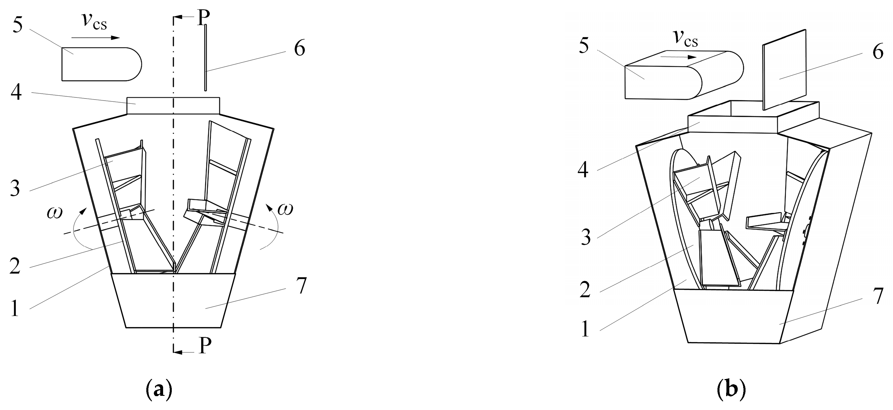
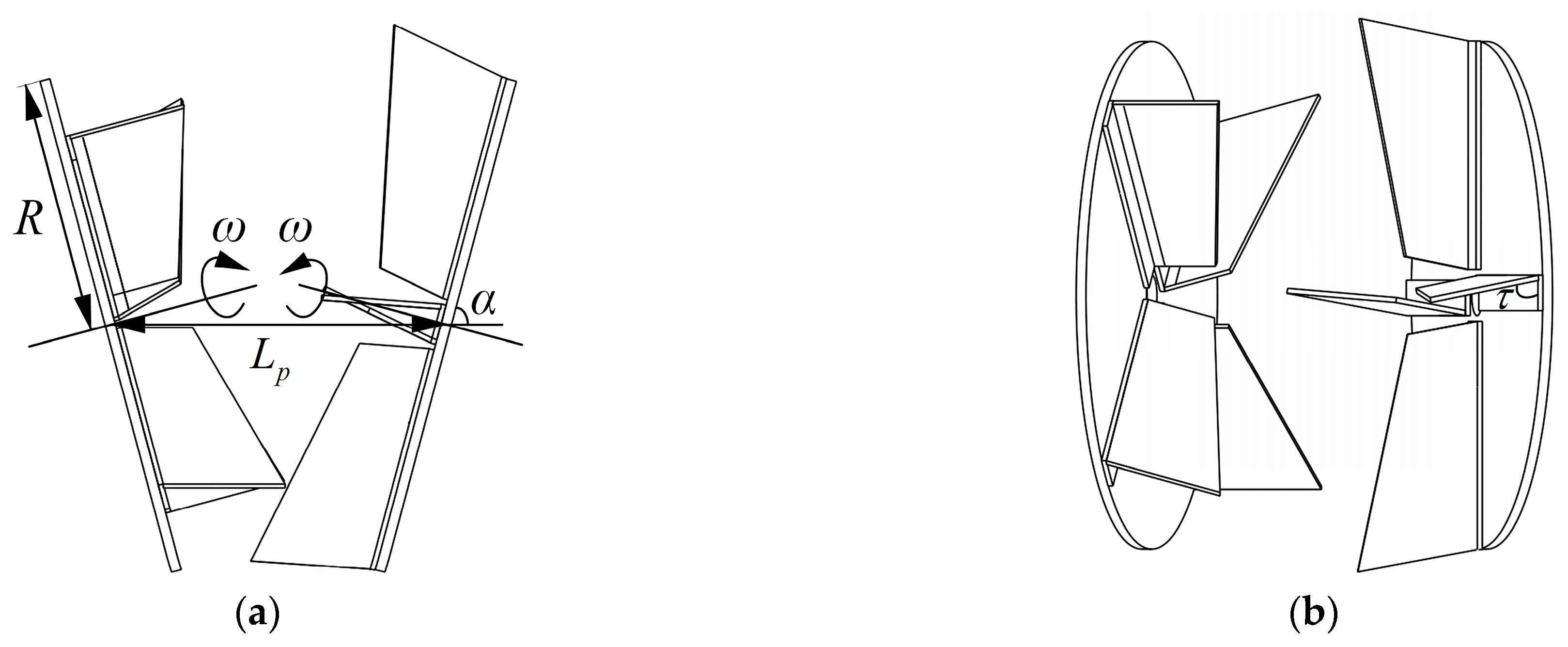
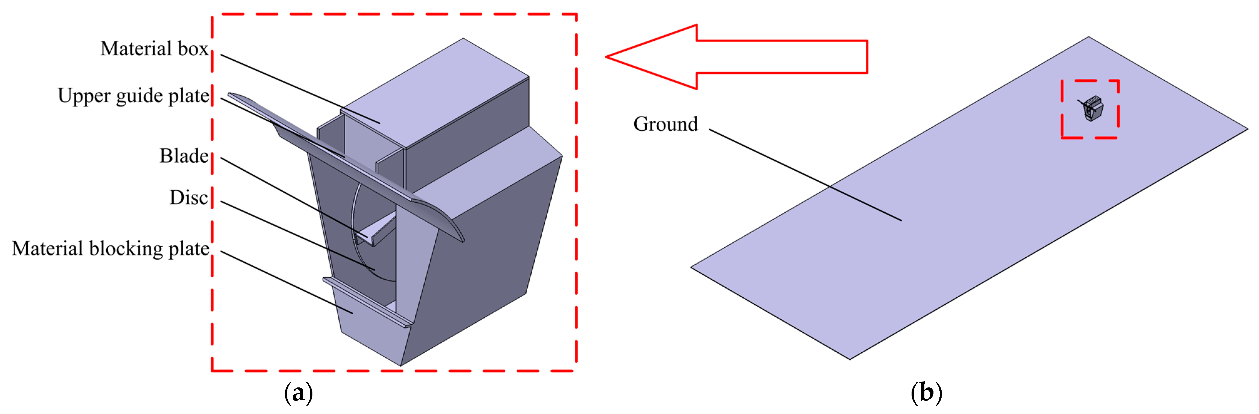
2.1. Structural Configuration and Operational Principles of Centrifugal Spreader

The tilted-disc organic fertilizer side-throwing centrifugal spreader structure is illustrated in Figure 1. It consists of (1) an ejection chamber, (2) two discs (the speed of the two discs is ω), (3) blades forming the main throwing unit, (4) a feed inlet, and (7) a material deflector. The feeding process is regulated by (5) a conveying device (the conveying speed is vcs) and (6) a feed control baffle.
Figure 2 demonstrates the working mechanism of the side-throwing centrifugal spreader. During operation, organic fertilizer falls through the feed inlet under the coordinated control of the conveying device and feed control baffle, subsequently landing on the high-speed rotating main throwing unit. The accelerated materials are then ejected through the outlet of the ejection chamber, forming a narrow-range, long-distance uniform side-throwing stream.
Structural parameters were extracted from the main throwing unit, as shown in Figure 3, to establish an accurate mathematical model of the material interaction with the main throwing unit.
Analysis of Figure 3 reveals that adjusting the blade–disc angle τ according to the disc inclination α can modify particle movement towards either the blade’s inner side (away from the disc) or outer side (adjacent to the disc), enabling the adjustment of stream divergence. The study focuses on the counter-tilted disc configuration in our team-designed side-throwing centrifugal spreader prototype.
Table 1 summarizes the model parameters, including the structural and operational specifications with corresponding symbols, dimensions, and value ranges.
As detailed in Table 1, the side-throwing centrifugal spreader prototype features are as follows:
Structural parameters:
  • Disc diameter (R): 500 mm;
  • Disc inclination angle (α): 75°;
  • Blade–disc angle (τ): 320 mm.
  • Operational parameters:
  • Disc rotation speed (ω): 700 rpm;
  • Machine travel speed (VNCC): 3.6 m/s;
  • Feed rate (mcs): 6 kg/s.
  • Material properties:
  • Particle mass (m): 4 × 10⁻⁴ kg;
  • Friction coefficient (kf): 0.11 (steel surface);
  • Gravitational acceleration (g): 9.81 m/s2.
The study investigated how adjusting τ affects the resultant force on particles, particle displacement along blades, and particle relative velocity to the throwing unit under these established parameters.

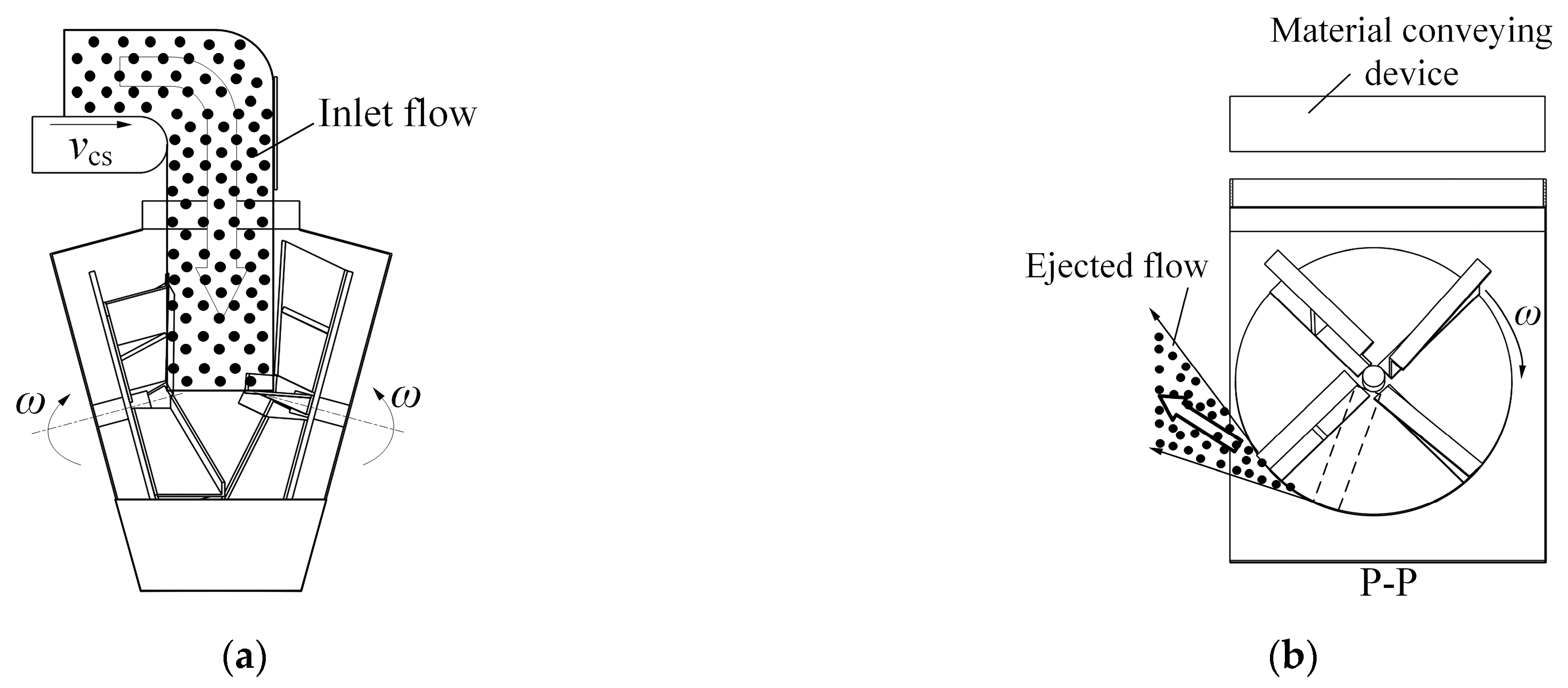
2.2. Theoretical Analysis of Organic Fertilizer Particle Projection by the Main Throwing Unit

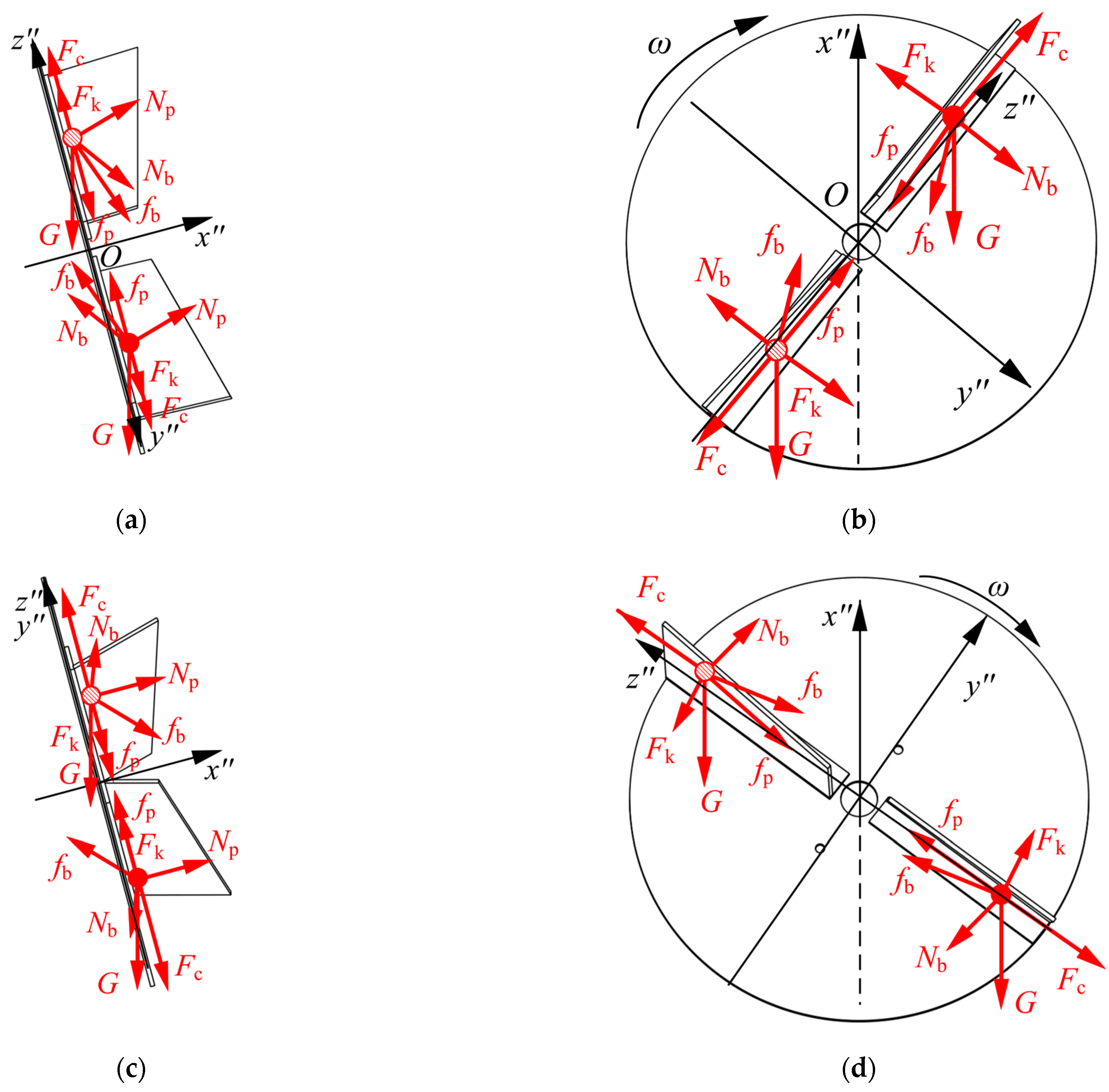
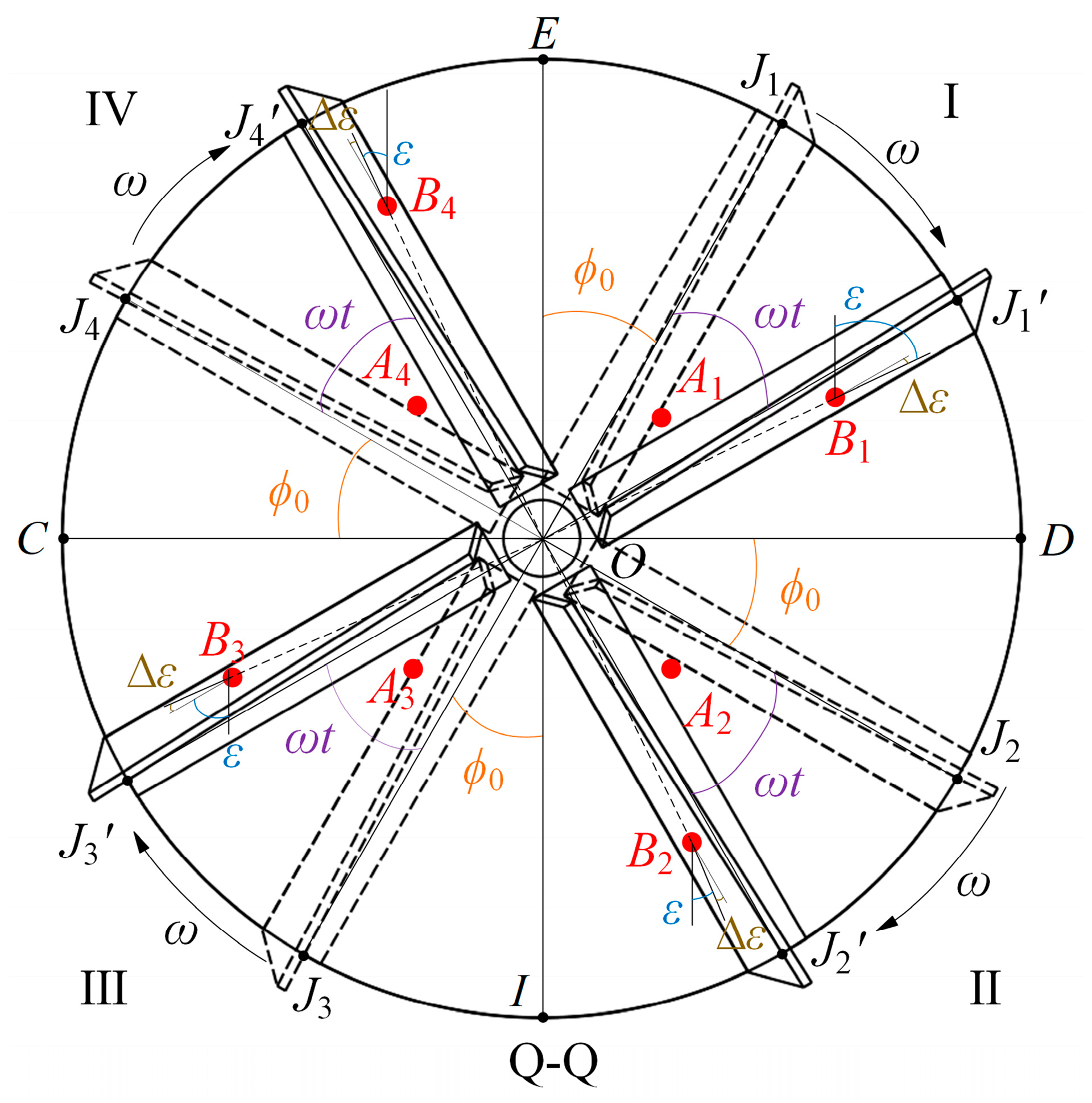
2.2.1. Reference Coordinate System Establishment

Taking the disc near the material feeding device as an example, in order to investigate the motion pattern of the material flow on the blade, it is necessary to establish spatial coordinate systems based on the machine body, the disc, and the blades, as shown in Figure 4. The blades are mathematically described, and the forces acting on the organic fertilizer particles are analyzed quadrant by quadrant.
Let the origin O be the center of the circular face of the disc, where the blades are mounted. The positive direction of the x-axis points towards the rear of the machine, and the positive direction of the z-axis is upwards. A y-axis is established perpendicular to the xOz-plane, with the positive direction of the y-axis pointing towards the direction of the thrown stream of material. The coordinate system O-xyz represents the base coordinate system of the entire machine.
Since the angle between the disc and the horizontal plane is α, the coordinate system O-xyz is rotated counterclockwise around the y-axis to obtain the disc’s coordinate system O-xyz′. In this system, the y′-axis and the z′-axis divide the disc into four quadrants. The rotation axis of the disc coincides with the x′-axis. The intersection of the disc’s outer contour and the z′-axis is represented by points E and I, while the intersection of the disc’s outer contour and the y′-axis is represented by points C and D. The regions EOD, DOI, COI, and COE are considered the first, second, third, and fourth quadrants, respectively.
To make the model more universally applicable, the primary working surface of the blade is treated as a standard plane, and a coordinate system O-xyz″ is established for the blade. In this system, the x″-axis coincides with the x′-axis, with both positive directions being aligned. The z″-axis is parallel to the long edge of the blade mounting plate, and its positive direction points towards the blade side of the disc’s center. The y″-axis is perpendicular to the xOz″-plane, with the positive direction of the y″-axis pointing in the direction of the blade’s rotational linear velocity. The coordinate system O-xyz″ rotates as the blade spins around the x″-axis at the same angular velocity as the disc. The coordinate system O-xyz″ represents the coordinate system of the blade in the second quadrant, as shown in Figure 4b.
Let any point on the plane where the working side of the blade is located in the coordinates of O-xyz″ be ( x 0 , y 0 , z 0 ), and let the plane over the O point from the non-working side of the blade point to the direction of the working side of the unit normal vector, the z″-axis points to the positive direction side of the right angle, the y″-axis points to the positive direction side of the angle of 90°−τ, and the x″-axis points to the positive direction side of the angle of τ; then, ( cos τ , sin τ , cos π 2 ) are the coordinates of this unit normal vector, meaning the blade plane equation is as follows:
cos τ x x 0 + sin τ y y 0 + cos π 2 z z 0 = 0

2.2.2. Kinematic and Dynamic Analysis of Particles Under Force

It is necessary to analyze both the variation in particle velocity and the resultant force acting on the particles during the spreading process in order to investigate the motion of organic fertilizer particles on the main throwing component of the lateral spreading device.
First, we examine the change in particle velocity on the main throwing component. Since the angle between the particle velocity vector and the coordinate system plane varies with time t, it is more convenient to express and calculate the vector quantities using their projections in a Cartesian coordinate system.
The absolute velocity VAC of an organic fertilizer particle on the disc can be regarded as the vector sum of the relative velocity VRC of the particle with respect to the main throwing component and the absolute velocity VNC of the main throwing component itself. The relative velocity VRC of the organic fertilizer particle with respect to the main throwing component is illustrated in Figure 5.
The velocity VNC is primarily composed of the rotational linear velocity of the disc combined with the forward velocity of the entire machine. The rotational linear velocity of the disc can be expressed as follows:
V NCZ = ω R
where R is the radius of the disc in meters.
The relative velocity Vrc of the organic fertilizer particle with respect to the main throwing component can be expressed as follows:
V rc = d L d t
where L is the path length of the particle relative to the main throwing component, m, and t is the time taken for the particle to traverse this path in seconds.
Assume the angle between L and the positive direction of the x″-axis is κ, the angle with the positive y″-axis is μ, and the angle with the positive z″-axis is ξ.
Let the angle between L and the positive direction of the x″-axis be κ, the angle between L and the positive direction of the y″-axis be μ, and the angle between L and the positive direction of the z″-axis be ξ. Let the projection of Vrc on the yOz″ plane be VrcyOz, and the projection of Vrc on the xOz″ plane be VrcxOz. The velocity Vrc of the organic fertilizer granules relative to the main throwing component can be vectorially represented as follows:
V rc = ( d L d t cos κ , d L d t cos μ , d L d t cos ξ )
The rotational linear velocity of the disc VNC can be expressed as a vector as follows:
V NC = ( 0 , ω R , 0 )
According to the size and direction of the force related to the organic fertilizer particles and the state of motion of the organic fertilizer particles, the force can be divided into two categories.
The first type of force has nothing to do with the state of motion of the organic fertilizer particles, that is, the size and direction of the force acting on the organic fertilizer particles in the process of movement are unchanged. Such forces include gravity G. The second type of force is related to the state of motion of the organic fertilizer particles, that is, such forces will be acting with the movement of the organic fertilizer particles to change the size and direction. Such forces include centrifugal force Fc, the support force Nb of the vane of the organic fertilizer particles, the friction fb of the blade on organic fertilizer particles, the support force Np acting on the organic fertilizer particles on the disc, the friction fp on the disc with the organic fertilizer particles, the Coriolis force Fk, and the force of the quadrant of the particles under analysis, as shown in Figure 6. The figure shows the situation when the particles are in close contact with the disc. When the particles are not in close contact with the disc, they are not subject to the supporting force Np or the frictional force fp exerted by the disc. The coordinate systems in Figure 6 are the coordinate systems of the blades in the first and fourth quadrants. The x″-axis direction of the coordinate system of the blade in the second quadrant is the same as that of the blade in the fourth quadrant, while the y″-axis and z″-axis directions are opposite. The x″-axis direction of the coordinate system of the blade in the third quadrant is the same as that of the blade in the first quadrant, while the y″-axis and z″-axis directions are opposite.
At present, the only force whose magnitude and direction can be determined is the gravitational force G. The magnitudes and directions of the other forces need to be determined through analyzing the motion state of the organic fertilizer particles. Therefore, the relative motion of the organic fertilizer particles with respect to the main throwing component is described, as shown in Figure 7.
Figure 7 is the Q-Q projection view of Figure 4a. This projection enables a more intuitive analysis of the motion of the organic fertilizer particles compared to other perspectives. In Figure 7, the motion state of the organic fertilizer particles is divided into quadrants, where OJ1, OJ2, OJ3, and OJ4 represent the positions of the blades when the organic fertilizer particles first contact the blades in quadrants I, II, III, and IV, respectively. Points A1, A2, A3, and A4 denote the initial positions at which the organic fertilizer particles land on the main throwing component in quadrants I, II, III, and IV, respectively. After time t, the blade positions change from OJ1, OJ2, OJ3, and OJ4 to OJ1′, OJ2′, OJ3′, and OJ4′, respectively, and the organic fertilizer particles move from points A1, A2, A3, and A4 to points B1, B2, B3, and B4, respectively. The angle through which the blades rotate is ωt.
Let the coordinates of the organic fertilizer particle in the O-xyz″ system be denoted as (x′, y′, z′), and the angle between the projection of the particle on the disc and the line from the origin O to the z″-axis can be calculated as follows:
Δ ε = arccos z 1 y 1 2 + z 1 2
Let point ( x 1 , y 1 , z 1 ) be projected onto the disc. If the line connecting this projection to the origin O forms a clockwise angle with the positive z″-axis, then ∆ε is defined as positive; if the angle is counterclockwise, then ∆ε is negative. Therefore, the quadrant division should be changed from the traditional coordinate axes y′ and z′ to a new division where the axes y′ and z′ rotate around the x′-axis by Δε. In this case, the EOD, DOI, COI, and COE regions are located in quadrant I, quadrant II, quadrant III, and quadrant IV, respectively. Since Δε depends on the shape of the blade’s surface and the position of the organic fertilizer particles, the quadrant division will change as the organic fertilizer particles move. For instance, the change in the quadrant of the organic fertilizer particle at point B is shown in Figure 2. Therefore, when discussing the force on the organic fertilizer particle at a certain point, it is necessary to first determine which quadrant the particle is currently in.
Let ε denote the angle between the centrifugal force acting on an organic fertilizer particle and its projection onto the segment EI (i.e., the z′-axis). When the particle is located in quadrant I, the angle ε is expressed as follows:
ε = ϕ 0 + ω t + Δ ε
where ε is the angle between the line segments OJ and OD at the moment when the organic fertilizer particle has just landed on its corresponding main throwing component, rad; the line segment OJ coincides with the z″-axis at this moment; and the angle is positive on the clockwise side of line segment OD, being negative otherwise.
When the particle is located in quadrant II, the angle ε is expressed as follows:
ε = π 2 ( ϕ 0 + ω t + Δ ε )
where ε is the angle between the line segments OJ and OD at the moment when the organic fertilizer particle has just landed on its corresponding main throwing component, in radians; the line segment OJ coincides with the z″-axis at this moment; and the angle is positive on the clockwise side of the line segment OD, being negative otherwise.
When the particle is located in quadrant III, the angle ε is expressed as follows:
ε = ϕ 0 + ω t + Δ ε
where ε is the angle between the line segments OJ and OI at the moment when the organic fertilizer particle has just landed on its corresponding main throwing component, in radians; the line segment OJ coincides with the z″-axis at this moment; and the angle is positive on the clockwise side of the line segment OI, being negative otherwise.
When the particle is located in quadrant IV, the angle ε is expressed as follows:
ε = π 2 ( ϕ 0 + ω t + Δ ε )
where ε is the angle between the line segments OJ and OC at the moment when the organic fertilizer particle has just landed on its corresponding main throwing component, in radians; the line segment OJ coincides with the z″-axis at this moment; and the angle is positive on the clockwise side of the line segment OC, being negative otherwise.
The absolute velocity of the organic fertilizer particle is expressed as follows:
V AC = V rc 2 + V NC 2
where Vrc is the relative velocity between the organic fertilizer particle and its corresponding main throwing component in m/s, and VNC is the absolute velocity of the main throwing component in m/s.
The velocity VNC is mainly composed of the superposition of the disc’s rotational linear velocity and the forward velocity of the machine. The disc’s rotational linear velocity can be expressed as follows:
V NC = ω R
where R is the radius of the disc in meters.
The relative velocity Vrc between the organic fertilizer particle and its primary throwing component can be expressed as follows:
V rc = d L d t
where L is the movement path of the organic fertilizer particle relative to the main throwing component in meters, and t is the time taken for the particle to move in seconds.
The resultant force Fr acting on the organic fertilizer particle can be expressed as follows:
F r = F c + G + F k + N p + N b + f p + f b
where Fr, Fc, G, Fc, Np, Nb, fp, and fb are the resultant force acting on the particle on the blade, the centrifugal force acting on the particle, the gravitational force acting on the particle, the Coriolis force, the support force exerted by the disc on the particle, the support force exerted by the blade on the particle, the frictional force exerted by the disc on the particle, and the frictional force exerted by the blade on the particle, respectively.

2.2.3. Establishment of Mechanical Equations for Organic Fertilizer Granules

Since the motion of the particle within the primary throwing component is continuous and the resultant force Fc acting on the particle at the current moment affects the relative velocity Vrc between the particle and the primary throwing component at the next moment, the current relative velocity Vrc also influences the force Fr acting on the particle at the current moment. Here, we define the time interval between successive moments as Δt, with Δt→0 s. At the n+1-th moment ( n = 0 , 1 , 2 , 3 , , n ), the equation for Vrcn+1 can be expressed as follows:
V rc n + 1 = V rc n + a n Δ t
where Vrcn is the relative velocity of the particle to its main throwing component at the n-th moment in m/s, and an is the acceleration of the particle at the n-th moment in m/s2.
The acceleration an of the particle at the n-th moment can be expressed as follows:
a n = F r n m
where Frn is the resultant force acting on the particle at the n-th moment in newtons, and m is the mass of the particle in kg.
Substituting Equation (16) into Equation (15) gives the following:
V rc n + 1 = V rc n + F r n m Δ t
where Vrcn+1 is the relative velocity of the organic fertilizer particle to its main throwing component at the (n+1)-th moment in m/s.
When the initial time t0 and the initial relative velocity Vrc0 are known, the relationship between the normal force Frn and the relative velocity Vrcn can be used to iteratively calculate the resultant force Fr acting on the granule and the relative velocity Vrc of the granule with respect to the main spreading component at any given moment.
An analysis of the resultant force acting on the granule is conducted, and the corresponding mechanical equations are established as follows.
Since the primary spreading region of the inclined disc, as the main component of the side-throwing device, lies within the third and fourth quadrants of the disc, the motion of the organic fertilizer granules in these quadrants and the associated mechanical equations are formulated and solved.
In cases where the granule is simultaneously supported by both the blade (support force Nb) and the disc (support force Np)—that is, when the granule is located in the gap between the disc and the blade—the blade’s tilt angle does not correct the trajectory of the organic fertilizer granules. Therefore, this scenario is excluded from the discussion, and only the case where the granule is not supported by the blade (Nb = 0) is considered.
When the particle is located in the third quadrant III, the equation is expressed as follows:
N b 3 = 2 m ω sin κ sin τ cos ξ sin κ d L d t + sin τ sin Δ ε m r ω 2 + m g cos τ cos α + sin τ sin α sin ϕ 0 + ω t
f b 3 = k f 2 m ω sin κ sin τ cos ξ sin κ d L d t + sin τ sin Δ ε m r ω 2 + m g cos τ cos α + sin τ sin α sin ϕ 0 + ω t
where Nb3 is the supporting force exerted by the blade on the particle in quadrant III, and fb131 is the frictional force exerted by the blade on the particle in quadrant III.
The unit vector of Nb3 is given by (cosτ, sinτ, 0), while the unit vector of fb3 is (−cosκ, −cosμ, −cosξ). The governing equation of motion along the x″-axis is expressed as follows:
m d 2 L cos κ d t 2 = 2 m ω cos τ sin κ sin τ cos ξ sin κ d L d t + m r ω 2 cos τ sin τ sin Δ ε + m g cos α + cos τ cos τ cos α + sin τ sin α sin ϕ 0 + ω t 2 m ω sin κ sin τ cos ξ sin κ d L d t + sin τ sin Δ ε m r ω 2 + m g cos τ cos α + sin τ sin α sin ϕ 0 + ω t k f cos κ
The governing equation of motion in the y″-axis direction is given by the following:
m d 2 L cos μ d t 2 = m r ω 2 sin Δ ε + sin 2 τ sin Δ ε + m g sin ϕ 0 + ω t sin α + sin τ cos τ cos α + sin τ sin α sin ϕ 0 + ω t + 2 m ω sin κ d L d t cos ξ sin κ + sin 2 τ cos ξ sin κ 2 m ω sin κ sin τ cos ξ sin κ d L d t + m r ω 2 sin τ sin Δ ε + m g cos τ cos α + sin τ sin α sin ϕ 0 + ω t k f cos μ
The governing equation of motion in the z″-axis direction is given by the following:
m d 2 L cos ξ d t 2 = m r ω 2 cos Δ ε + m g cos ϕ 0 + ω t sin α 2 m ω sin κ cos μ sin κ d L d t k f cos ξ 2 m ω sin κ sin τ cos ξ sin κ d L d t + m r ω 2 sin τ sin Δ ε + m g cos τ cos α + sin τ sin α sin ϕ 0 + ω t
When the particle is located in the fourth quadrant IV, the equation is expressed as follows:
N b 4 = 2 m ω sin κ sin τ cos ξ sin κ d L d t + m r ω 2 sin τ sin Δ ε + m g cos τ cos α + sin τ sin α cos ϕ 0 + ω t
f b 4 = k f 2 m ω sin κ sin τ cos ξ sin κ d L d t + m r ω 2 sin τ sin Δ ε + m g cos τ cos α + sin τ sin α cos ϕ 0 + ω t
where Nb4 is the supporting force exerted by the blade on the particle in quadrant IV, while fb4 is the frictional force exerted by the blade on the particle in the fourth quadrant.
The unit vector of Nb4 is given by (cosτ, sinτ, 0), while the unit vector of fb4 is (−cosκ, −cosμ, −cosξ). The governing equation of motion along the x″-axis is expressed as follows:
m d 2 L cos κ d t 2 = 2 m ω cos τ sin κ sin τ cos ξ sin κ d L d t + m r ω 2 cos τ sin τ sin Δ ε + m g cos α + cos τ cos τ cos α + sin τ sin α cos ϕ 0 + ω t k f cos κ 2 m ω sin κ sin τ cos ξ sin κ d L d t + m r ω 2 sin τ sin Δ ε + m g cos τ cos α + sin τ sin α cos ϕ 0 + ω t
The governing equation of motion in the y″-axis direction is given by the following:
m d 2 L cos μ d t 2 = m r ω 2 sin Δ ε + sin Δ ε sin 2 τ + m g cos ϕ 0 + ω t sin α + sin τ cos τ cos α + sin τ sin α cos ϕ 0 + ω t + 2 m ω sin κ d L d t cos ξ sin κ + sin 2 τ cos ξ sin κ k f cos μ 2 m ω sin κ sin τ cos ξ sin κ d L d t + m r ω 2 sin τ sin Δ ε + m g cos τ cos α + sin τ sin α cos ϕ 0 + ω t
The governing equation of motion in the z″-axis direction is given by the following:
m d 2 L cos ξ d t 2 = m r ω 2 cos Δ ε m g sin ϕ 0 + ω t sin α 2 m ω sin κ cos μ sin κ d L d t k f cos ξ 2 m ω sin κ sin τ cos ξ sin κ d L d t + m r ω 2 sin τ sin Δ ε + m g cos τ cos α + sin τ sin α cos ϕ 0 + ω t

2.3. Analytical Solution of the Mechanical Equations

The mechanical equations are solved separately for cases where the particle is located in quadrants III and IV. When the particle is in quadrant III, the initial conditions are as follows:
t = 0 L = 0 d L d t = 0
Solve the mechanical Equation (20) for the particle along the x″-axis, and let
λ 1 = ( k f cos κ cos τ ) 2 ω cos τ sin τ cos ξ + ( k f cos κ cos τ ) 2 ω cos τ sin τ cos ξ 2 4 cos κ k f cos κ cos τ ω 2 cos τ sin τ sin Δ ε 2 cos κ λ 2 = ( k f cos κ cos τ ) 2 ω cos τ sin τ cos ξ ( k f cos κ cos τ ) 2 ω cos τ sin τ cos ξ 2 4 cos κ k f cos κ cos τ ω 2 cos τ sin τ sin Δ ε 2 cos κ K 1 = r 0 ω 2 sin τ sin Δ ε cos τ k f cos κ g cos α + cos τ k f cos κ g cos τ cos α U 1 = k f cos κ cos τ ω 2 sin τ sin Δ ε J 1 = cos τ k f cos κ g sin τ sin α W 1 = ω 2 sin τ sin Δ ε cos τ k f cos κ ω 2 cos κ V 1 = ( k f cos κ cos τ ) 2 ω 2 sin τ cos ξ R 1 = K 1 U 1 W 1 J 1 sin ϕ 0 V 1 J 1 cos ϕ 0 W 1 2 + V 1 2 P 1 = ω W 1 J 1 cos ϕ 0 + V 1 J 1 sin ϕ 0 W 1 2 + V 1 2 C 1 = P 1 λ 2 R 1 λ 1 λ 2 C 2 = λ 1 R 1 P 1 λ 1 λ 2
The general solution of the mechanical equation for the particle along the x″-axis is as follows:
L ¯ = C 1 e λ 1 t + C 2 e λ 2 t
The particular solution is as follows:
L = L ¯ + L = C 1 e λ 1 t + C 2 e λ 2 t + K 1 U 1 + W 1 J 1 sin ϕ 0 V 1 J 1 cos ϕ 0 W 1 2 + V 1 2 cos ω t + W 1 J 1 cos ϕ 0 + V 1 J 1 sin ϕ 0 W 1 2 + V 1 2 sin ω t
To solve the mechanical Equation (21) for the particle along the y″-axis, let
λ 3 = ( 1 + k f cos μ sin τ sin 2 τ ) 2 ω cos ξ + ( 1 + k f cos μ sin τ sin 2 τ ) 2 ω cos ξ 2 4 cos μ k f cos μ sin τ sin 2 τ 1 ω 2 sin Δ ε 2 cos μ λ 4 = ( 1 + k f cos μ sin τ sin 2 τ ) 2 ω cos ξ ( 1 + k f cos μ sin τ sin 2 τ ) 2 ω cos ξ 2 4 cos μ k f cos μ sin τ sin 2 τ 1 ω 2 sin Δ ε 2 cos μ K 2 = r 0 ω 2 sin Δ ε sin 2 τ + 1 k f cos μ sin τ + g cos τ cos α sin τ k f cos μ U 2 = k f cos μ sin τ sin 2 τ 1 ω 2 sin Δ ε J 2 = sin τ k f cos μ sin τ 1 g sin α W 2 = ω 2 sin Δ ε k f cos μ sin τ sin 2 τ 1 ω 2 cos μ V 2 = ( 1 + k f cos μ sin τ sin 2 τ ) 2 ω 2 cos ξ R 2 = K 2 U 2 W 2 J 2 sin ϕ 0 V 2 J 2 cos ϕ 0 W 2 2 + V 2 2 P 2 = ω W 2 J 2 cos ϕ 0 + V 2 J 2 sin ϕ 0 W 2 2 + V 2 2 C 3 = P 2 λ 4 R 2 λ 3 λ 4 C 4 = λ 3 R 2 P 2 λ 3 λ 4
The general solution of the mechanical equation for the particle along the y″-axis is as follows:
L ¯ = C 3 e λ 3 t + C 4 e λ 4 t
The particular solution is as follows:
L = L ¯ + L = C 3 e λ 3 t + C 4 e λ 4 t + K 2 U 2 + W 2 J 2 sin ϕ 0 V 2 J 2 cos ϕ 0 W 2 2 + V 2 2 cos ω t + W 2 J 2 cos ϕ 0 + V 2 J 2 sin ϕ 0 W 2 2 + V 2 2 sin ω t
To solve the mechanical Equation (22) for the particle along the y″-axis, let
λ 5 = ( k f cos 2 ξ sin τ + cos μ ) 2 ω + ( k f cos 2 ξ sin τ + cos μ ) 2 ω 2 4 cos ξ k f cos ξ sin τ sin Δ ε cos Δ ε ω 2 2 cos ξ λ 6 = ( k f cos 2 ξ sin τ + cos μ ) 2 ω ( k f cos 2 ξ sin τ + cos μ ) 2 ω 2 4 cos ξ k f cos ξ sin τ sin Δ ε cos Δ ε ω 2 2 cos ξ K 3 = r 0 ω 2 cos Δ ε k f cos ξ sin τ sin Δ ε k f cos ξ g cos τ cos α U 3 = k f cos ξ sin τ sin Δ ε cos Δ ε ω 2 J 3 = g sin α cos ϕ 0 k f cos ξ g sin τ sin α sin ϕ 0 Q 3 = g sin α sin ϕ 0 k f cos ξ g sin τ sin α cos ϕ 0 W 3 = ω 2 k f cos ξ sin τ sin Δ ε cos Δ ε ω 2 cos ξ V 3 = ( k f cos 2 ξ sin τ + cos μ ) 2 ω 2 R 3 = K 3 U 3 W 3 J 3 V 3 Q 3 W 3 2 + V 3 2 P 3 = ω W 3 J 3 + V 3 Q 3 W 3 2 + V 3 2 C 5 = K 3 λ 6 R 3 λ 5 λ 6 C 6 = λ 5 R 3 K 3 λ 5 λ 6
The general solution of the mechanical equation for the particle along the z″-axis is as follows:
L ¯ = C 5 e λ 5 t + C 6 e λ 6 t
The particular solution is as follows:
L = L ¯ + L = C 5 e λ 5 t + C 6 e λ 6 t + K 3 U 3 + W 3 J 3 V 3 Q 3 W 3 2 + V 3 2 cos ω t + W 3 J 3 + V 3 Q 3 W 3 2 + V 3 2 sin ω t
When the particle is in quadrant IV, the initial conditions are as follows:
t = 0 L = 0 d L d t = 0
Solve the mechanical Equation (25) for the particle along the x″-axis, and let
λ 7 = ( k f cos κ cos τ ) 2 ω cos τ sin τ cos ξ + ( k f cos κ cos τ ) 2 ω cos τ sin τ cos ξ 2 4 cos κ k f cos κ cos τ ω 2 cos τ sin τ sin Δ ε 2 cos κ λ 8 = ( k f cos κ cos τ ) 2 ω cos τ sin τ cos ξ ( k f cos κ cos τ ) 2 ω cos τ sin τ cos ξ 2 4 cos κ k f cos κ cos τ ω 2 cos τ sin τ sin Δ ε 2 cos κ K 4 = r 0 ω 2 sin τ sin Δ ε cos τ k f cos κ g cos α + cos τ k f cos κ g cos τ cos α U 4 = k f cos κ cos τ ω 2 sin τ sin Δ ε U 4 = k f cos κ cos τ ω 2 sin τ sin Δ ε J 4 = cos τ k f cos κ g sin τ sin α W 4 = ω 2 sin τ sin Δ ε cos τ k f cos κ ω 2 cos κ V 4 = ( k f cos κ cos τ ) 2 ω 2 sin τ cos ξ R 4 = K 4 U 4 W 4 J 4 cos ϕ 0 + V 4 J 4 sin ϕ 0 W 4 2 + V 4 2 cos ω t K 4 = ω W 4 J 4 sin ϕ 0 + V 4 J 4 cos ϕ 0 W 4 2 + V 4 2 cos ω t C 7 = K 4 λ 8 R 4 λ 7 λ 8 C 8 = λ 7 R 4 K 4 λ 7 λ 8
The general solution of the mechanical equation for the particle along the x″-axis is as follows:
L ¯ = C 7 e λ 7 t + C 8 e λ 8 t
The particular solution is as follows:
L = L ¯ + L = C 7 e λ 7 t + C 8 e λ 8 t + K 4 U 4 + W 4 J 4 cos ϕ 0 + V 4 J 4 sin ϕ 0 W 4 2 + V 4 2 cos ω t + W 4 J 4 sin ϕ 0 + V 4 J 4 cos ϕ 0 W 4 2 + V 4 2 sin ω t
To solve the mechanical Equation (26) for the particle along the y″-axis, let
λ 9 = ( 1 + k f cos κ sin τ sin 2 τ ) 2 ω cos ξ + ( 1 + k f cos κ sin τ sin 2 τ ) 2 ω cos ξ 2 4 cos μ k f cos μ sin τ sin 2 τ 1 ω 2 sin Δ ε 2 cos μ λ 10 = ( 1 + k f cos κ sin τ sin 2 τ ) 2 ω cos ξ ( 1 + k f cos κ sin τ sin 2 τ ) 2 ω cos ξ 2 4 cos μ k f cos μ sin τ sin 2 τ 1 ω 2 sin Δ ε 2 cos μ K 5 = r 0 ω 2 sin Δ ε sin 2 τ + 1 k f cos μ sin τ + g cos τ cos α sin τ k f cos μ U 5 = k f cos μ sin τ sin 2 τ 1 ω 2 sin Δ ε J 5 = sin τ k f cos μ sin τ 1 g sin α W 5 = ω 2 sin Δ ε k f cos μ sin τ sin 2 τ 1 ω 2 cos μ V 5 = ( 1 + k f cos μ sin τ sin 2 τ ) 2 ω 2 cos ξ R 5 = K 5 U 5 W 5 J 5 cos ϕ 0 + V 5 J 5 sin ϕ 0 W 5 2 + V 5 2 cos ω t K 5 = ω W 5 J 5 sin ϕ 0 + V 5 J 5 cos ϕ 0 W 5 2 + V 5 2 cos ω t C 9 = K 5 λ 10 R 5 λ 9 λ 10 C 10 = λ 9 R 5 K 5 λ 9 λ 10
The general solution of the mechanical equation for the particle along the y″-axis is as follows:
L ¯ = C 9 e λ 9 t + C 10 e λ 10 t
The particular solution is as follows:
L = L ¯ + L = C 9 e λ 9 t + C 10 e λ 10 t + K 5 U 5 + W 5 J 5 cos ϕ 0 + V 5 J 5 sin ϕ 0 W 5 2 + V 5 2 cos ω t + W 5 J 5 sin ϕ 0 + V 5 J 5 cos ϕ 0 W 5 2 + V 5 2 sin ω t
To solve the mechanical Equation (27) for the particle along the z″-axis, let
λ 11 = ( k f cos 2 ξ sin τ + cos μ ) 2 ω + ( k f cos 2 ξ sin τ + cos μ ) 2 ω 2 4 cos ξ k f cos ξ sin τ sin Δ ε cos Δ ε ω 2 2 cos ξ λ 12 = ( k f cos 2 ξ sin τ + cos μ ) 2 ω ( k f cos 2 ξ sin τ + cos μ ) 2 ω 2 4 cos ξ k f cos ξ sin τ sin Δ ε cos Δ ε ω 2 2 cos ξ K 6 = r 0 ω 2 cos Δ ε k f cos ξ sin τ sin Δ ε k f cos ξ g cos τ cos α U 6 = k f cos ξ sin τ sin Δ ε cos Δ ε ω 2 J 6 = g sin α sin ϕ 0 k f cos ξ g sin τ sin α cos ϕ 0 Q 6 = g sin α cos ϕ 0 k f cos ξ g sin τ sin α sin ϕ 0 W 6 = ω 2 k f cos ξ sin τ sin Δ ε cos Δ ε ω 2 cos ξ V 6 = ( k f cos 2 ξ sin τ + cos μ ) 2 ω 2 R 6 = K 6 U 6 W 6 J 6 V 6 Q 6 W 6 2 + V 6 2 cos ω t K 6 = ω W 6 J 6 + V 6 Q 6 W 6 2 + V 6 2 cos ω t C 11 = K 6 λ 12 R 6 λ 11 λ 12 C 12 = λ 11 R 6 K 6 λ 11 λ 12
The general solution of the mechanical equation for the particle along the z″-axis is as follows:
L ¯ = C 11 e λ 11 t + C 12 e λ 12 t
The particular solution is as follows:
L = L ¯ + L = C 11 e λ 11 t + C 12 e λ 12 t + K 6 U 6 + W 6 J 6 V 6 Q 6 W 6 2 + V 6 2 cos ω t + W 6 J 6 + V 6 Q 6 W 6 2 + V 6 2 sin ω t

2.4. Virtual Simulation

2.4.1. Simulation Model Development

Since the ejection flow patterns generated by the dual-side discs of the side-throw device are identical and symmetrical with respect to the central axis of the device, and because the ejection flows from both sides may overlap during operation, it becomes difficult to directly measure and analyze the overlapping regions in the simulation software. Therefore, the simulation adopts a fixed-point ejection approach using a single-sided disc. After obtaining the ejection flow generated by the single disc, a symmetrical overlay is applied to reconstruct the ejection flow pattern produced by the dual-disc system. The ejection patterns of both the single- and dual-disc configurations are analyzed to examine how the fertilizer-scraping blades correct the trajectories of material particles.
First, a three-dimensional model of the side-throw device is created. Structural components irrelevant to the simulation results are simplified without affecting the accuracy of the simulation. The simplified side-throw model is shown in Figure 8a. To observe the particle trajectory correction effect after ejection more clearly, a ground model for fixed-point ejection is established, as shown in Figure 8b.

2.4.2. Simulation Parameter Settings

In the discrete element simulation software EDEM 2020, the intrinsic and contact parameters of the commercial eco-organic fertilizer used in the experiment were applied as measured in the preliminary tests. The particle diameter for the simulation was selected according to the particle size distribution and mass fraction of the organic fertilizer. Given the approximately spherical shape of organic fertilizer particles, basic spheres were adopted as the geometric model.
When configuring the particle factory parameters, organic fertilizer particles were generated within corresponding size ranges according to the measured particle size distribution. The median value of each size range was used as the simulated particle diameter (with the size range exceeding 5 mm specifically set to 5 mm). Particle factories were established based on a uniform distribution within these size ranges to ensure that the simulated particle distribution closely approximated that of the actual organic fertilizer particles.
To balance computational efficiency and simulation authenticity, the simulation domain size was set to five times the average particle diameter of the actual organic fertilizer. The corresponding mass fractions are provided in Table 2.
The physical properties of the material, steel, and soil, along with the contact parameters between them, are shown in Table 3 [19,27].
The three-dimensional model is imported into the EDEM 2020 software, which automatically generates a simulation domain based on the model’s dimensions, as shown in Figure 9.
In Figure 9, the red rectangular wireframe represents the computational domain, and the coordinate system within the frame serves as the reference coordinate system for the simulation environment. The X-axis, Y-axis, and Z-axis correspond to the depth direction, horizontal direction, and vertical direction, respectively. Due to the adhesive nature of the material and soil, which leads to significant bonding and aggregation, the contact models for the material-to-material, material-to-soil, and soil-to-soil interactions are all defined using the Hertz–Mindlin with the JKR model. Furthermore, as the material tends to adhere to the side-throwing device, the contact model between the material and the side-throwing device is also set to the Hertz–Mindlin with the JKR model [28,29,30]. Additionally, since the fertilizer makes contact with the soil upon landing during actual spreading operations, simulations should replicate this real-world soil interaction. Early-stage investigations revealed negligible differences between two simulation approaches: modeling a ground surface with physical soil particles versus assigning soil properties directly to the ground plane. Both methods produced identical simulation trends, yet assigning soil properties to the ground plane significantly accelerated the computational speed. Consequently, this study employed this method, defining contact parameters between the fertilizer and soil to more accurately simulate post-spreading effects [19]. The particle factory is placed inside the hopper and set to a dynamic type, with a particle generation rate of 6 kg/s. The total simulation duration was 6.5 s divided into the following two phases. Particle generation and natural accumulation (0–2 s): A baffle was used to prevent particles from falling during generation, allowing them to naturally accumulate while simulating the adhesive behavior of organic fertilizer particles under static conditions. Feeding and throwing (2–6.5 s): The baffle was removed, enabling the particles to fall freely into the throwing chamber where they were dispersed by the main throwing component. The disc operates at a rotational speed of 700 rpm, and the rotation occurs between 2 and 6.5 s. A fixed time step of 0.00015 s is applied, with data being recorded at intervals of 0.01 s.

2.5. Experimental Setup and Testing

2.5.1. Experimental Setup and Materials

The experiment was conducted on 20 October 2023 at Northeast Agricultural University in the Xiangfang District of Harbin, Heilongjiang Province. The weather was clear, with temperatures ranging from 21 °C to 25 °C, a north wind, and wind speeds between 2 and 4 km/h. The experimental material used was commercial ecological organic fertilizer produced by Yilirong Agricultural Technology Co., Ltd. (Harbin, China).
The experimental setup consisted of two main components: a feed hopper and a side-throwing device. The side-throwing device includes an inclined, counter-rotating disc equipped with blades, along with auxiliary components and additional mechanisms, as shown in Figure 10. During the experiment, the disc was operated at a rotational speed of 700 rpm, with a feed rate of 6 kg/s, and the throwing duration was set to 10 s.

2.5.2. Experimental Methodology

The experiments were conducted using blades with inclination angles of 65°, 70°, 75°, 80°, and 85°. The blades were installed every 90° to align with the center of the disc. A fixed-point throwing method was employed for the experiment. Prior to the tests, a wind speed meter was used to measure the wind speed and direction at the experimental site. The first experiment served as the baseline, and subsequent experiments were conducted under the same wind speed and direction as the initial test. The wind speed was measured using the PROVA AVM-01 anemometer (Prova AG, Zurich, Switzerland), with a measurement error of less than 5% for each test. A Seiko SQ5540C stopwatch (Seiko Epson Corporation, Tokyo, Japan) was used for timing. A Stanley 33–252 FatMax tape measure (The Stanley Works, New Britain, CT, USA) was used to measure the distance.
Before the experiment, the material feed chain was shut off, and the rotational speed of the disc was measured using the SMART SENSOR AR971 tachometer (Shenzhen Smart Sensor Technology Co., Ltd., Shenzhen, China). The disc speed was adjusted to 500, 700, and 900 rpm (with a measurement error of less than 5% for each test). Based on the set feed rate, the required size of the discharge opening was calculated, and the material feed chain was activated to complete the feeding and throwing process.
During the throwing process, the scattering angle of the jet stream in the air was captured through photography and analyzed to evaluate the effect of the blade inclination angle on material correction. After the throwing was completed, the effective throwing distance of the device was measured. Each experiment was repeated three times, and the averages of the three sets of data were taken to observe the variation pattern.
To ensure accurate measurement of scattering angles, the raw images were processed using MATLAB R2021b through the following sequence: (1) grayscale conversion, (2) image preprocessing, (3) edge detection with the Canny operator, (4) contour extraction, (5) linear curve fitting of the extracted contours, and (6) scattering angle calculation. The measurement approach is illustrated in Figure 11.

3. Results

3.1. Numerical Analysis

Let the particle mass m, the disc inclination angle α, the coefficient of sliding friction between the particle and the steel surface kf, and the disc rotational speed ω be 4 × 10⁻⁴ kg, 75°, 0.11, and 700 rpm, respectively. Preliminary experiments indicated that the particle’s motion on the blade structure, with the given experimental parameters, lasts no longer than 0.025 s. Based on the initial conditions, Equations (28) and (38), as well as the analytical solutions (31), (34), (37), (41), (44), and (47), a mathematical model describing the particle’s motion on the disc blades was established and solved using a MATLAB R2021b-based solver. The resulting motion patterns of the particle on blades with different inclination angles over the time interval from 0 to 0.025 s are shown in Figure 12.

3.2. Virtual Simulation Evaluation Index Measurement Methods

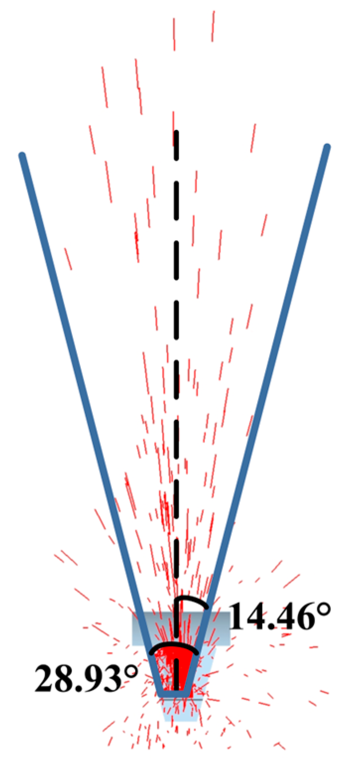
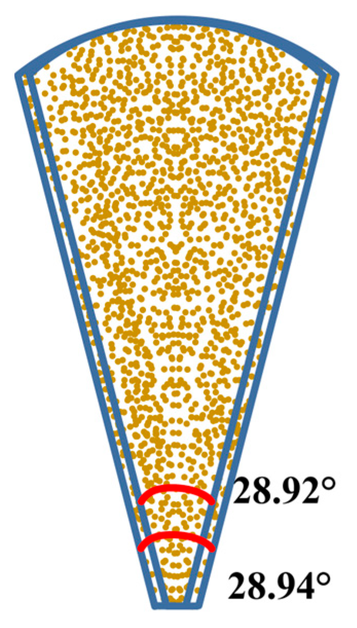
3.2.1. Jet Flow Pattern Analysis

The influence of the blade–disc angle on particle trajectory correction is analyzed from a macroscopic perspective by observing the divergence of the jet flow. Specifically, the scattering angle of the single-sided disc jet in the air is measured and analyzed. Taking the disc on the side closer to the hopper as an example, the morphology of the jet flow produced by blades at angles between 70° and 90° at the same time point (1 s into spreading) is shown in Figure 13.
From Figure 13, it can be observed that, as the blade angle increases, the jet flow gradually diverges. The scattering angle formed by the single-sided disc is defined by the inner edge line on the inner side of the device and the outer edge line on the outer side. The angle between the inner edge line of the scattering angle and the vertical direction ranges from −9.92° to 9.12° (in Figure 13, the angle on the right side of the vertical line is negative, while the left side is positive). The scattering angle decreases progressively from 25.81° to 19.69°. It can be seen from analyzing Figure 13 that the outer edge line of the scattering angle formed by the single-sided disc jet flow diverges outward, but at a slower rate than the inner edge line. The specific variation curve is shown in Figure 13f.
The jet flow section obtained from Figure 13 is symmetrically mirrored around the device’s central axis, resulting in the complete jet flow section for the double-sided disc, as shown in Figure 14.
From Figure 14, it can be seen that when the blade angle is within the range from 70° to 90°, a separation phenomenon occurs in the jet flow of both discs when the blade angle exceeds 80°. The separation angle increases as the blade angle increases. When the blade angle is 90°, the separation angle reaches its maximum value of 18.24°. When the blade angle is less than 80°, an overlap phenomenon occurs in the jet flow of both discs, with the overlap angle increasing as the blade angle decreases. When the blade angle is 70°, the overlap angle reaches its maximum value of 19.84°. The overall scattering angle of the jet flow from both discs increases with the blade angle. When the blade angle is 70°, the scattering angle is at its minimum value of 31.80°, while at 90°, it is at its maximum value of 57.62°. In this context, the overlap angle of the jet flow from both discs is negative, and the separation angle is positive. The curves depicting the scattering angles of the jet flows from the double-sided discs, as well as the overlap and separation angles, are shown in Figure 13f.
Upon further analysis of Figure 14f, it can be observed that when the jet flows of both discs overlap, the overall scattering angle is minimized. By continuing to reduce the blade angle, it is found that when the blade angle is 65°, the angles between the inner and outer edge lines of the jet flow formed by the single-sided disc and the vertical direction are equal, as shown in Figure 15. The jet flow section obtained from Figure 15 is symmetrically mirrored around the device’s central axis, resulting in the complete jet flow section for the double-sided disc, as shown in Figure 16.

3.2.2. Particle Trajectory Analysis on the Blade

The motion of a single particle on the blade was analyzed during the calibration of blade inclination angles ranging from 65° to 85°. The selected particle did not undergo collisions or adhesion with other particles and was influenced solely by the blade. Additionally, the particle exhibited a clear motion trajectory on the blade surface rather than being directly ejected upon contact. The velocity components of the particle along each coordinate axis were recorded. The influence of the blade–disc angle on particle motion correction can be quantitatively assessed at the microscopic level by examining the velocity variations in this single particle. The particle velocity profiles are shown in Figure 17.

3.3. Analysis of Experimental Results

The measured scattering angles and effective throwing distances were statistically analyzed, and the trends are illustrated in Figure 18 and Figure 19. As shown in Figure 18, within the blade inclination range from 65° to 85°, the scattering angle of the jet stream increases monotonically with the blade angle. This trend remains consistent when changing the disc rotational speed, and the disc rotational speed has a relatively small impact on the scattering angle. When the disc rotational speed is 900 rpm and the blade tilt angle is 65°, the minimum scattering angle is 26.41°. When the disc rotational speed is 500 rpm and the blade tilt angle is 85°, the maximum scattering angle reaches 57.87°. This trend is attributed to the gradual divergence of the jet streams formed by the two discs: As the blade inclination increases, the initially overlapping jet streams begin to separate. When the blade angle reaches 85°, the streams become fully separated, forming a distinct separation angle. This pattern is consistent with the trend observed in Figure 14.
Figure 19 shows that the effective throwing distance of the jet stream first increases and then decreases as the blade inclination increases within the range from 65° to 85°. When the blade inclination angle is 80°, the effective range of the jet is the largest. Changing the disc rotation speed maintains this trend, but it has a significant impact on the value of the effective throwing distance. When the rotation speed reaches 900 rpm and the blade inclination angle is 80°, the maximum effective range of the jet can reach 12.0 m. When the rotation speed is 500 rpm and the blade inclination angle is 65°, the minimum effective range of the jet is 6.2 m. This phenomenon is attributed to the fact that as the disc rotation speed increases, the absolute velocity of the particles increases; therefore, the impact on the effective throwing distance is more significant. When the blade inclination angle is 80°, the velocity of the particles in the forward direction is the largest. Therefore, at the same rotation speed, the effective throwing distance is the farthest when the blade inclination angle is 80°. This pattern is consistent with the trend observed in Figure 17.

4. Discussion

4.1. Mathematical Modeling and Numerical Analysis

In constructing the mathematical model and conducting numerical analysis, the MATLAB code adopts the time-stepping iterative structure of the explicit Euler method. It calculates the forces in the three axis directions, using mechanical equations to update the velocity and displacement. At the same time, it uses constraint optimization (lsqnonlin to solve the least-squares problem with boundary constraints) to dynamically determine the angular parameters so as to simulate the motion trajectory of a particle in three-dimensional space. Error analysis of the mathematical model and numerical simulation process revealed that the primary source of error is the force composition phase. Due to the extensive use of exponential and trigonometric functions in the mechanical equations—the values of which are predominantly non-terminating, non-repeating decimals—numerous approximations are introduced during computation. Additionally, a certain degree of error accumulates during the time integration process. Collectively, these factors contribute to an error margin of 5–10%. In subsequent research, the author aims to refine the mathematical model and numerical analysis procedures by increasing the integration accuracy, optimizing the time step size, and improving the non-linear solving techniques, thereby reducing the overall error.
As shown in Figure 12a, at 0.025 s, with an increase in the blade inclination angle, the particle’s velocity along the x″-axis first decreases and then increases. When the blade inclination angle reaches 80°, the particle’s velocity along the x″-axis is minimized, approaching zero. According to Figure 12b, at 0.025 s, as the blade inclination angle increases, the particle’s velocity along the y″-axis first increases and then decreases. When the blade inclination angle is 80°, the particle’s velocity along the y″-axis is maximized at 6.5 m/s. Figure 12c shows that at 0.025 s, with the increase in the blade inclination angle, the particle’s velocity along the z″-axis first increases and then decreases. When the blade inclination angle reaches 80°, the particle’s velocity along the z″-axis is maximized at 18.7 m/s. As shown in Figure 12d, at 0.025 s, with the increase in blade inclination angle, the particle’s overall velocity first increases and then decreases. When the blade inclination angle is 80°, the particle’s overall velocity is maximized at 19.8 m/s. Therefore, it is concluded that the optimal blade inclination angle for both simulation and experimental setups is 80° and that the blade inclination angle range is between 70° and 90°. Two parameters, namely, the Disc Inclination Angle and Angle Between Center-Mounted Blades and Disc, were incorporated, distinguishing this study from previous works [22,23,24]. By introducing these parameters, the model’s versatility is enhanced, leading to a more intricate particle movement trajectory and heightened research complexity.

4.2. Discrete Element Simulation

Based on the variation curves in Figure 14f and the analysis of Figure 15 and Figure 16, it can be concluded that when the blade angle is 65°, the jet flow sections from both discs tend to overlap. At this point, the overall scattering angle of the combined jet flow from the two discs is 28.94°. By incorporating the angle data obtained from Figure 15 and Figure 16 into Figure 13f and Figure 14f, the updated trend curves are presented in Figure 20 and Figure 21.
From the trend curves of single-disc jet flow parameters in Figure 20, it is observed that within the blade angle range from 65° to 90°, the scattering angle of the single-disc jet flow decreases monotonically with the increasing blade angle, reducing from 28.93° to 19.69°. Meanwhile, the angle between the inner edge line of the single-disc jet flow and the vertical direction increases monotonically with the blade angle, rising from −14.46° to 9.12°.
According to the trend curves of double-disc jet flow parameters in Figure 21, the most convergent jet flow occurs when the blade angle is 65°, with a scattering angle of 28.94°, while the most divergent jet flow appears at a blade angle of 90°, with a scattering angle of 57.62°. The difference in scattering angles between these two extremes is 28.68°.
In summary, the blade angle serves as an effective parameter for controlling the divergence and convergence of the jet flow.
After the simulation, the effective throwing distance of the blade spread surface at various angles was measured, and the results are shown in Figure 22.
As shown in Figure 22, with the increase in the blade inclination angle, the effective throwing distance on one side of the spreading disc first increases and then decreases. The maximum effective throwing distance, 10.8 m, occurs at a blade inclination of 80°, while the minimum, 9.1 m, is observed at an inclination of 65°.
As observed in Figure 17, the particle remains in contact with the blade for approximately 0.025 s. After this period, its velocity stabilizes, indicating that it is no longer influenced by the blade. During the interaction, the particle’s velocity along the X- and Z-axes initially increases and then decreases with the increase in blade inclination. The maximum velocities along both axes occur at a blade inclination of 80°, with the X-axis reaching 18.5 m/s and the Z-axis reaching 8.1 m/s.
In contrast, the Y-axis velocity of the particle exhibits a more complex pattern with changing blade inclinations. In the interval of 0–0.005 s, particles on blades of all inclination angles accelerate toward the inner side of the device. Between 0.005 and 0.010 s, particles on the 85° blade begin to decelerate toward the inner side, while those on other blades continue to accelerate inward. From 0.010 to 0.015 s, particles on the 80° blade decelerate inward, while those on the 85° blade accelerate outward; particles on the remaining blades continue to accelerate inward. In the 0.015–0.020 s interval, particles on both the 80° and 85° blades accelerate outward, whereas particles on other blades maintain inward acceleration. During the 0.020–0.025 s period, particles on the 80° blade decelerate outward and eventually reduce their velocity to 0 m/s; particles on the 85° blade continue to accelerate outward but with decreasing acceleration, resulting in velocity stabilization. Particles on the other blades also accelerate inward with diminishing acceleration, leading to velocity stabilization.
This analysis reveals that while changes in blade inclination significantly affect the magnitude of particle velocity along the X- and Z-axes, they do not alter the overall trend of these components. However, blade inclination has a notable impact on both the trend and magnitude of Y-axis velocity. The X and Z components of velocity primarily determine the effective throwing distance of the overall jet stream, while the Y component governs its divergence or convergence. Therefore, it is possible to effectively manipulate particle trajectories to regulate both the scattering angle and effective throwing distance of the jet by adjusting the blade inclination.
As shown in Figure 12 and Figure 17, when the blade inclination is 65°, the particle exhibits the lowest absolute velocity upon leaving the blade. As the inclination increases to 80°, the absolute velocity increases accordingly, reaching a maximum. When the blade inclination exceeds 80°, the absolute velocity begins to decrease, which is consistent with the trend observed in Figure 22 for the effective throwing distance.
This study delves into the dynamics of macroscopic ejection and microscopic particle velocity within discrete element virtual simulations, contrasting with the existing literature [25,26]. It establishes correlations between the changing trends of microscopic particle velocity and macroscopic ejection through mathematical models and prototype experiments.

4.3. Experimental Testing

A comprehensive analysis of Figure 18 and Figure 19 indicates that within the blade inclination range from 65° to 80°, the scattering angle of the jet stream increases with the blade angle, while the effective throwing distance also increases. However, in the range from 80° to 85°, although the scattering angle continues to increase, the effective throwing distance gradually decreases. A comparison between Figure 10 and Figure 18, as well as Figure 19 and Figure 22, shows that the scattering angles and effective throwing distances obtained from the prototype tests deviate from the simulation results by less than 10%, and the overall trends are consistent. This confirms the accuracy of the simulation.
Due to the necessary simplification of the mathematical model and the trade-off of research strategies, at this current stage, the interactions between the same particles are not described. These interactions between particles will be examined in future studies, and the mathematical model will subsequently be supplemented and improved. The current investigation focuses on exploring the impact of the Angle Between Center-Mounted Blades and Disc on particle trajectory due to the limited test cycles. Future research will extend this analysis to include the influence of the blade installation angle on particle trajectory to enhance the comprehensiveness of the mathematical model. The simulation software EDEM 2020 used in this study lacks the capability to incorporate air resistance into macroscopic ejection simulations, suggesting potential enhancement through EDEM-Fluent coupled simulations. Furthermore, future research will necessitate testing in controlled laboratory settings and large-scale agricultural environments to ensure the practical applicability of the findings.

5. Conclusions

This study investigates the impact of the Angle Between Center-Mounted Blades and Disc on particle trajectory through mutual validation of numerical calculations, discrete element simulations, and prototype experiments.
(1)
The spatial coordinate system established with the blade as the reference frame, which rotates with the disc, can describe the complex relative motion of particles on the blade under the dual inclination of the disc and the blade. By analyzing the forces and motion of particles in each quadrant during the particle throwing process on the inclined disc, a mathematical model describing the force acting on the particles by the main throwing components is obtained. This model can describe the resultant force acting on the particles on the blade at any given moment. By further deriving the model equations, it becomes possible to qualitatively and quantitatively calculate the displacement, velocity, and force variation in particles on the blade when parameters such as disc inclination, disc rotational speed, blade mounting angle, and blade inclination are known.
(2)
When the particle mass m = 4 × 10⁻⁴ kg, the disc inclination α = 75°, the sliding friction coefficient between the particle and the steel surface kf = 0.4, and the disc rotational speed ω = 700 rpm, after 0.025 s of motion on the blade, the change in particle velocity for different blade inclinations demonstrates that adjusting the blade inclination can effectively correct the motion trajectory of the particles on the blade.
(3)
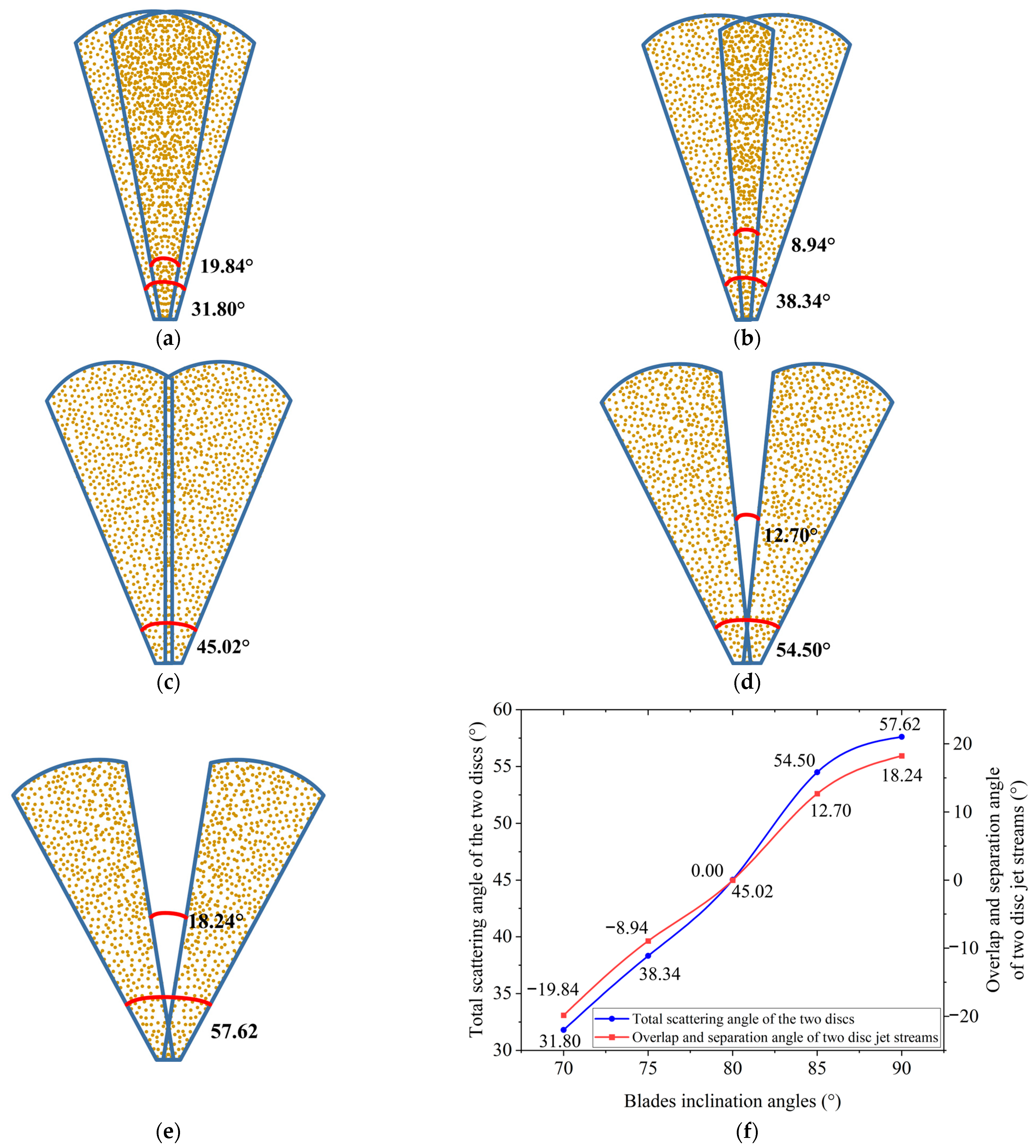
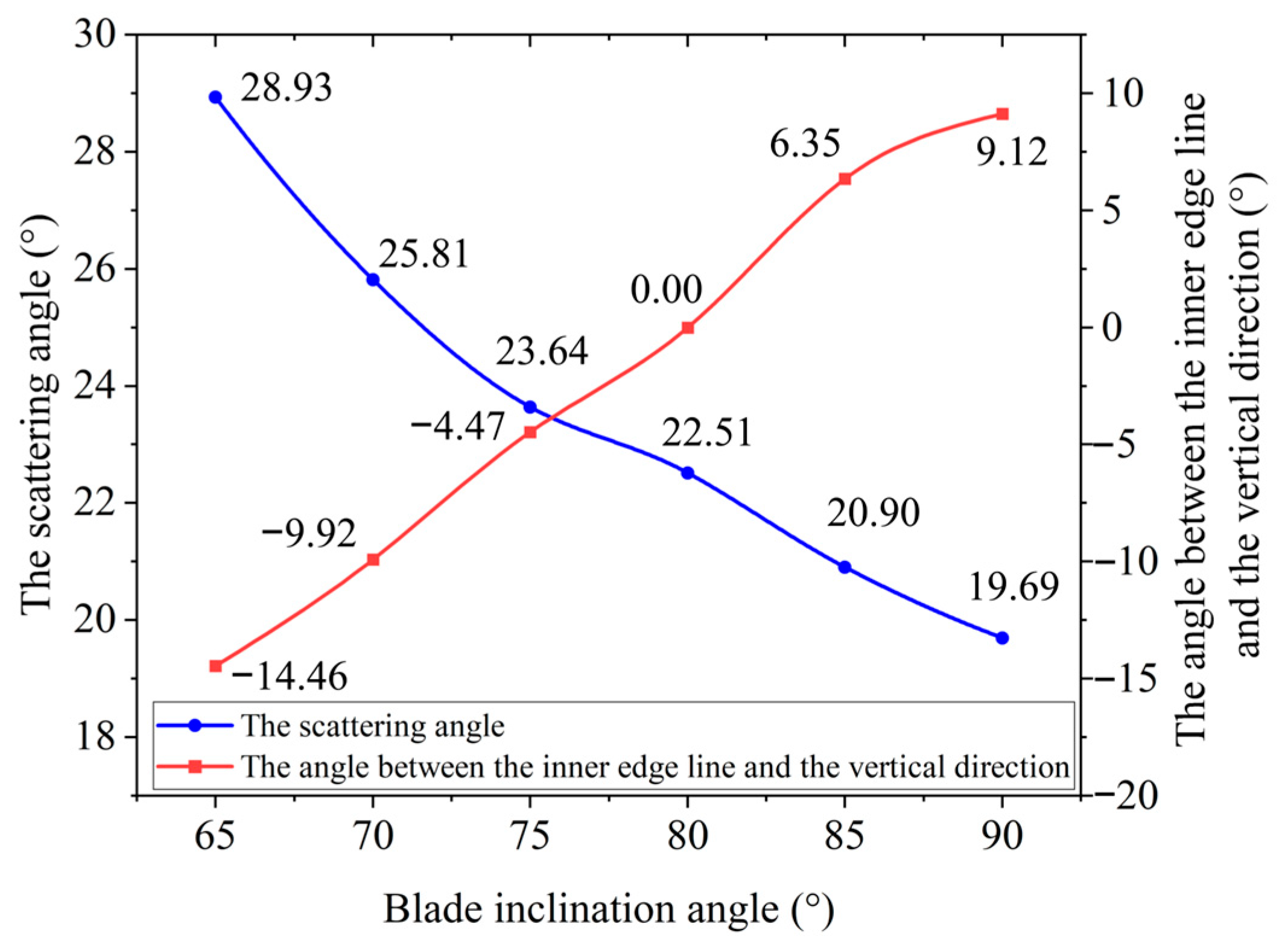
For a side-throwing device with a disc radius of 500 mm, disc inclination of 75°, center-to-center distance between the two discs of 320 mm, disc rotational speed of 700 rpm, and blades mounted concentrically, within the blade inclination range from 65° to 85°, as the blade inclination increases, the scattering angle of the jet stream formed by the single disc gradually decreases, while the scattering angle of the overall jet stream formed by both discs gradually increases. The jet streams from the two discs transition from crossing to separation. When the blade inclination is 65°, the jet streams from both discs nearly overlap, and at an inclination of 80°, the jet streams from both discs approach the critical point of overlap and separation.
(4)
For the same side-throwing device, when the blade inclination range is between 65° and 85°, the device with a 65° blade produces the minimum scattering angle for the overall jet stream formed by both discs, the smallest absolute velocity when the particles leave the blade, and the shortest effective throwing distance on the distribution surface. The device with an 80° blade produces the maximum absolute velocity when the particles leave the blade and the longest effective throwing distance. The device with an 85° blade results in the largest scattering angle for the overall jet stream formed by both discs. Changing the disc rotation speed does not alter the above trends, and it has a non-significant impact on the scattering angle but a significant impact on the effective throwing distance. The mathematical model, virtual simulation, and prototype testing corroborate each other, further clarifying that the blade inclination can influence the overall jet stream morphology by correcting the particle motion path on the blade. This not only lays a foundation for further exploring the control capabilities of the inclined disc side-throwing device in terms of jet stream morphology, but also presents a universal mathematical framework and methodology applicable to centrifugal spreading systems in various engineering fields.

Author Contributions

Conceptualization, Y.X.; methodology, Y.X.; software, Y.X.; validation, H.L. and J.S.; formal analysis, Y.X. and H.L.; investigation, H.L. and L.G.; resources, Y.X.; data curation, Y.X. and J.S.; writing—original draft preparation, Y.X.; writing—review and editing, H.L. and L.G.; visualization, J.S., L.G. and G.Z.; supervision, J.S.; project administration, J.S.; funding acquisition, H.L. and G.Z. All authors have read and agreed to the published version of the manuscript.

Funding

This research was financially supported by the Subproject of Heilongjiang Provincial Key Research and Development Program (No. 2022ZX02C14-1).

Institutional Review Board Statement

Not applicable.

Data Availability Statement

The original contributions presented in this study are included in the article. Further inquiries can be directed to the corresponding author.

Conflicts of Interest

The authors declare no conflicts of interest.

References

  1. Fan, C.S.; He, R.Y.; Shi, Y.Y.; He, L.N. Structure and operation mode of centrifugal side-throwing organic fertilizer spreader for greenhouses. Powder Technol. 2024, 438, 119457. [Google Scholar] [CrossRef]
  2. Li, A.Q.; Jia, F.G.; Chu, Y.H.; Han, Y.L.; Li, H.; Sun, Z.; Ji, S.Y.; Li, Z.Z. Simulation of the movement of rice grains in a centrifugal huller by discrete element method and the influence of blade shape. Biosyst. Eng. 2023, 236, 54–70. [Google Scholar] [CrossRef]
  3. Sharipov, G.M.; Heiß, A.; Eshkabilov, S.L.; Griepentrog, H.W.; Paraforos, D.S. Considering field topography in the model-based assessment of a centrifugal spreader’s variable rate application accuracy. Comput. Electron. Agric. 2023, 213, 108234. [Google Scholar] [CrossRef]
  4. Gerakari, M.; Mitkou, D.; Antoniadis, C.; Giannakoula, A.; Stefanou, S.; Hilioti, Z.; Chatzidimopoulos, M.; Tsiouni, M.; Pavloudi, A.; Xynias, I.N.; et al. Evaluation of Commercial Tomato Hybrids for Climate Resilience and Low-Input Farming: Yield and Nutritional Assessment Across Cultivation Systems. Agronomy 2025, 15, 929. [Google Scholar] [CrossRef]
  5. Zinkevičienė, R.; Jotautienė, E.; Juostas, A.; Comparetti, A.; Vaiciukevičius, E. Simulation of granular organic fertilizer application by centrifugal spreader. Agronomy 2021, 11, 247. [Google Scholar] [CrossRef]
  6. Kömekçi, F.; Kömekçi, C.; Doğu, D.; Aykas, E. Effects of number of vanes, vane angle and disc peripheral speed on the distribution uniformity of twin-disc granular fertilizer broadcaster. Heliyon 2024, 10, 18. [Google Scholar] [CrossRef]
  7. Li, L.; Peng, L.; Zhao, W. Effects of process parameters on the spreading morphology of disc surface and aluminium powder produced by centrifugal atomisation. Powder Metall. 2023, 66, 509–518. [Google Scholar] [CrossRef]
  8. Wen, Y.J.; Zhang, J.C.; Yang, N.; Wang, X.H.; Shi, X.Y.; Wang, J.L. Effects of the long-term application of organic fertilization and straw returning on the components of soil organic carbon and pores. Trans. Chin. Soc. Agric. Eng. (Trans. CSAE) 2024, 40, 74–81, (In Chinese with English Abstract). [Google Scholar] [CrossRef]
  9. Jiao, J.C.; An, X.H.; Xu, C.X.; Li, T.L.; Meng, H.S.; Zhang, J.; Hao, X.J. Effects of organic fertilizer combined with Pseudomonas fluorescein on maize yield and phosphorus activity in reclaimed soil. Trans. Chin. Soc. Agric. Eng. (Trans. CSAE) 2024, 40, 79–87, (In Chinese with English Abstract). [Google Scholar] [CrossRef]
  10. Deng, S.S.; Yan, H.F.; Zhang, C.; Wang, G.Q.; Zhang, J.Y.; Liang, S.W.; Jiang, J.H. Effects of irrigation amounts and nitrogen reduction combined with organic fertilizer pattern on greenhouse cucumber and soil. Trans. Chin. Soc. Agric. Eng. (Trans. CSAE) 2023, 39, 93–102, (In Chinese with English Abstract). [Google Scholar] [CrossRef]
  11. Zhu, X.H.; Li, H.C.; Li, X.D.; Liang, J.H.; Zang, J.J.; Zhao, H.S.; Guo, W.C. Mechanized ring-furrow fertilization of organic fertilizers in orchards. Trans. Chin. Soc. Agric. Eng. (Trans. CSAE) 2023, 39, 60–70, (In Chinese with English Abstract). [Google Scholar] [CrossRef]
  12. Chen, G.B.; Wang, Q.J.; Li, H.W.; He, J.; Lu, C.Y.; Zhang, X.Y. Design and experiment of solid organic fertilizer crushing and striping machines. Trans. Chin. Soc. Agric. Eng. (Trans. CSAE) 2023, 39, 13–24, (In Chinese with English Abstract). [Google Scholar] [CrossRef]
  13. Wang, Y.; Tan, Y.; Zeng, S.; Zeng, H.; Zhao, Z.; Li, L.; Zhang, J.; Liu, W.; Ying, Z. Design and experimental study of the fertilizer applicator with vertical spiral fluted rollers. Int. J. Agric. Biol. Eng. 2023, 16, 80–87. [Google Scholar] [CrossRef]
  14. Bivainis, V.; Jotautienė, E.; Lekavičienė, K.; Mieldažys, R.; Juodišius, G. Theoretical and Experimental Verification of Organic Granular Fertilizer Spreading. Agriculture 2023, 13, 1135. [Google Scholar] [CrossRef]
  15. Guan, Z.H.; Mu, S.L.; Jiang, T.; Li, H.T.; Zhang, M.; Wu, C.Y.; Jin, M. Development of Centrifugal Disc Spreader on Tracked Combine Harvester for Rape Undersowing Rice Based on DEM. Agriculture 2022, 12, 562. [Google Scholar] [CrossRef]
  16. Sharipov, G.M.; Heiß, A.; Eshkabilov, S.L.; Griepentrog, H.W.; Paraforos, D.S. Variable rate application accuracy of a centrifugal disc spreader using ISO 11783 communication data and granule motion modeling. Comput. Electron. Agric. 2021, 182, 106006. [Google Scholar] [CrossRef]
  17. Hwang, S.J.; Nam, J.S. DEM simulation model to optimise shutter hole position of a centrifugal fertiliser distributor for precise application. Biosyst. Eng. 2021, 204, 326–345. [Google Scholar] [CrossRef]
  18. Liu, H.X.; Du, C.L.; Yin, L.W.; Zhang, G.F. Shooting flow shape and control of organic fertilizer sidethrowing on inclined opposite discs. Trans. Chin. Soc. Agric. Mach. 2022, 53, 168–177, (In Chinese with English Abstract). [Google Scholar] [CrossRef]
  19. Liu, H.X.; Zhao, Y.J.; Xie, Y.T.; Zhang, Y.M.; Shang, J.J. Design and experiment of spiral blades auxiliary roller of organic fertilizer side throwing device. Trans. Chin. Soc. Agric. Mach. 2023, 54, 107–119, (In Chinese with English Abstract). [Google Scholar] [CrossRef]
  20. Liu, H.X.; Wang, C.; Wang, J.X.; Fu, L.L. Design and experiment study on portable in-vehicle device of farmyard manure collecting. J. Northeast. Agric. Univ. 2017, 48, 59–71+96, (In Chinese with English Abstract). [Google Scholar] [CrossRef]
  21. Liu, H.X.; Wang, J.X.; Su, H.; An, J.Y. Design on side type discharge organic fertilizer spreader with inclined opposite discs and research on its key components. J. Northeast Agric. Univ. 2018, 49, 83–90+98, (In Chinese with English Abstract). [Google Scholar] [CrossRef]
  22. Cerović, V.B.; Petrović, D.V.; Radojević, R.L.; Barać, S.R.; Vuković, A. On the fertilizer particle motion along the vane of a centrifugal spreader disc assuming pure sliding of the particle. J. Agric. Sci. 2018, 63, 83–97. [Google Scholar] [CrossRef]
  23. Tomantschger, K.; Petrović, D.V.; Cerović, V.B.; Dimitrijević, Ž.A.; Radojević, R.L. Prediction of a fertilizer particle motion along a vane of a centrifugal spreader disc assuming its pure rolling. FME Trans. 2018, 46, 544–551. [Google Scholar] [CrossRef]
  24. Martínez-Rodríguez, A.; Gómez-Águila, M.V.; Soto Escobar, M. Model and Software for the Parameters Calculation in Centrifugal Disk of Fertilizer Spreaders. Rev. Cienc. Técnicas Agropecu. 2021, 30, 82–101. [Google Scholar]
  25. Zhang, G.Z.; Wang, Y.; Liu, H.P.; Ji, C.; Hou, Q.X.; Zhou, Y. Design and experiments of the centrifugal side throwing fertilizer spreader for lotus root fields. Trans. Chin. Soc. Agric. Eng. (Trans. CSAE) 2018, 34, 21–27, (In Chinese with English Abstract). [Google Scholar] [CrossRef]
  26. Liu, C.L.; Zhang, F.Y.; Du, X.; Jiang, M.; Yuan, H.; Liu, Q. Design and experiment of precision fertilizer distribution mechanism with horizontal turbine blades. Trans. Chin. Soc. Agric. Mach. 2020, 51, 165–174, (In Chinese with English Abstract). [Google Scholar] [CrossRef]
  27. Zeng, Z.W.; Ma, X.; Cao, X.L.; Li, Z.H.; Wang, X.C. Critical review of applications of discrete element method in agricultural engineering. Trans. Chin. Soc. Agric. Mach. 2021, 52, 1–20, (In Chinese with English Abstract). [Google Scholar] [CrossRef]
  28. Qi, Z.Y.; Liu, C.L.; Wang, Y.; Zhang, Z.W.; Sun, X.B. Design and Experimentation of Targeted Deep Fertilization Device for Corn Cultivation. Agriculture 2024, 14, 1645. [Google Scholar] [CrossRef]
  29. Huan, X.L.; Li, S.B.; Wang, L.; Wang, D.C.; You, Y. Study on silage mixing device of King Grass stalk particles based on DEM simulation and bench test. Powder Technol. 2024, 437, 119581. [Google Scholar] [CrossRef]
  30. Chen, G.; Wang, Q.; Li, H.; He, J.; Lu, C.; Xu, D.; Sun, M. Experimental research on a propeller blade fertilizer transport device based on a discrete element fertilizer block model. Comput. Electron. Agric. 2023, 208, 107781. [Google Scholar] [CrossRef]
Figure 1. Structure of the side-throwing device. (a) Front view. (b) Axis side view.
Agriculture 15 01392 g001
Figure 2. Working principle of the side-throwing device. (a) Front view. (b) P-P cross-section view.
Agriculture 15 01392 g002
Figure 3. Structural parameters of the main throwing component. (a) Front view. (b) Top view.
Agriculture 15 01392 g003
Figure 4. Reference coordinate system and quadrant division. (a) Front view. (b) Side view. I–IV refer to quadrant numbering.
Agriculture 15 01392 g004
Figure 5. Velocity analysis of organic fertilizer particles. (a) Front view of particle velocity in quadrants I and III. (b) Side view of particle velocity in quadrants I and III. (c) Front view of particle velocity in quadrants II and IV. (d) Side view of particle velocity in quadrants II and IV.
Agriculture 15 01392 g005
Figure 6. Force analysis of organic fertilizer particles. (a) Front view of particle forces in quadrants I and III. (b) Side view of particle forces in quadrants I and III. (c) Front view of particle forces in quadrants II and IV. (d) Side view of particle forces in quadrants II and IV.
Agriculture 15 01392 g006
Figure 7. Movement analysis of organic fertilizer particles. I–IV refer to quadrant numbering. Identical colors represent angles of the same type/category, consistently applied throughout all quadrants.
Agriculture 15 01392 g007
Figure 8. Simulation model of the side-throwing device. (a) Simplified model of the side-throwing device. (b) Ground model.
Agriculture 15 01392 g008
Figure 9. EDEM simulation environment.
Agriculture 15 01392 g009
Figure 10. Structural diagram of the experimental apparatus. (a) Front view of the complete spreader. (b) Front view of the side-throwing device. (c) Axial side view of the side-throwing device.
Agriculture 15 01392 g010
Figure 11. Method of measuring the scattering angle.
Agriculture 15 01392 g011
Figure 12. Motion patterns of particles moving on blades at various inclination angles. (a) The x′′-axis velocity component of particles moving on blades at various inclination angles. (b) The y′′-axis velocity component of particles moving on blades at various inclination angles. (c) The z′′-axis velocity component of particles moving on blades at various inclination angles. (d) The velocity of particles moving on blades at various inclination angles.
Agriculture 15 01392 g012
Figure 13. Ejection flow patterns of materials ejected from blades at various inclination angles on a single disc. (a) A 70° blade ejection flow. (b) A 75° blade ejection flow. (c) An 80° blade ejection flow. (d) An 85° blade ejection flow. (e) A 90° blade ejection flow. (f) Curves of the scattering angle and inner edge line position changes.
Agriculture 15 01392 g013
Figure 14. Ejection flow patterns of materials ejected from blades at various inclination angles on dual discs. (a) A 70° blade ejection flow. (b) A 75° blade ejection flow. (c) An 80° blade ejection flow. (d) An 85° blade ejection flow. (e) A 90° blade ejection flow. (f) Curves of the scattering angle and relative position changes in ejection flows between the two discs.
Agriculture 15 01392 g014
Figure 15. Ejection flow of a single disc with a 65° blade.
Agriculture 15 01392 g015
Figure 16. Ejection flow of dual discs with a 65° blade.
Agriculture 15 01392 g016
Figure 17. Particle velocity on blades at various inclination angles. (a) Particle velocity along the X-axis. (b) Particle velocity along the Y-axis. (c) Particle velocity along the Z-axis.
Agriculture 15 01392 g017
Figure 18. Variation in scattering angles for blades at different inclination angles.
Agriculture 15 01392 g018
Figure 19. Variation in the effective throwing distance of the material ejected by blades at different inclination angles in prototype tests.
Agriculture 15 01392 g019
Figure 20. Updated curves of the scattering angle and inner edge line position changes for the ejection flow of a single disc.
Agriculture 15 01392 g020
Figure 21. Updated curves of the scattering angle and relative position changes in ejection flows between dual discs.
Agriculture 15 01392 g021
Figure 22. Variation in the effective throwing distance of the material ejected by blades at different tilt angles in the virtual simulation.
Agriculture 15 01392 g022
Table 1. Structural parameters and operating parameters of the main throwing components.
ParameterSymbolDimensionValue (Range)
Organic fertilizer particle massmkg4 × 10−4
Friction coefficient between the fertilizer particle and the main throwing componentkf 0.11
Gravitational accelerationgm·s−29.81
Disc diameterRmm500
Disc tilt angleα°75
Angle between the blade and the discτ°65–90
Distance between the centers of two discsLpmm320
Disc rotation speedωrpm700
Machine travel speedVNCCm·s−13.6
Feed rate of the material conveying devicemcskg·s−16
Table 2. Particle size and mass fraction of the discrete element model of organic fertilizer granules.
Actual Particle Size (mm)Simulated Particle Size (mm)Mass Fraction (%)
0.00–0.501.2541.60
0.50–1.003.7526.15
1.00–2.007.5015.15
2.00–5.0012.5014.40
>5.00252.70
Table 3. Basic parameters of EDEM simulation.
ItemParameterValue
FertilizerPoisson’s ratio0.4
Shear modulus (Pa)2 × 10⁶
Density (kg·m−3)800
SteelPoisson’s ratio0.31
Shear modulus (Pa)7 × 10¹⁰
Density (kg·m−3)7900
SoilPoisson’s ratio0.3
Shear modulus (Pa)5 × 10⁷
Density (kg·m−3)2600
Fertilizer–fertilizerCoefficient of restitution0.6
Coefficient of static friction0.65
Coefficient of rolling friction0.1
Surface energy (J·m−2)0.45
Fertilizer–steelCoefficient of restitution0.6
Coefficient of static friction0.7
Coefficient of rolling friction0.11
Surface energy (J·m−2)0.0225
Fertilizer–soilCoefficient of restitution0.4
Coefficient of static friction0.66
Coefficient of rolling friction0.18
Surface energy (J·m−2)0.6
Disclaimer/Publisher’s Note: The statements, opinions and data contained in all publications are solely those of the individual author(s) and contributor(s) and not of MDPI and/or the editor(s). MDPI and/or the editor(s) disclaim responsibility for any injury to people or property resulting from any ideas, methods, instructions or products referred to in the content.

