Study on the Impact of Pipe Installation Height on the Hydraulic Performance of Combined Canal–Pipe Water Conveyance Systems

Abstract

This study investigates the impact of pipe installation height on the hydraulic performance of a combined canal–pipe water conveyance system (CCPS) and provides practical recommendations. A combined experimental and numerical simulation approach was conducted to systematically analyze and evaluate the impact of different pipe installation heights (0, 1, 3, and 5 cm) and flow rates (18.40, 21.21, 24.74, 28.27, 33.58, and 38.88 L/s) on the system’s behavior. The results indicated that the canal water depths obtained from the numerical simulations were in close agreement with the measurements from the experiments. The water depth in the upstream canal remained nearly parallel to the canal bottom. At the junction, the trend of water depth varies under different flow rates. When the flow rate is low, the water depth sharply decreases. Conversely, when the flow rate is higher, the water depth rises significantly. Cross sections farther from the junction exhibit a higher uniformity in flow velocity distribution. As the height of the pipe installation increases, the range of influence of the junction on the flow velocity distribution in the upstream canal decreases. The elevation of the pipe installation height has been instrumental in enhancing the uniformity of flow velocity distribution across the section. However, the local head loss gradually increases as the installation height increases. Turbulent kinetic energy (TKE) and turbulent eddy dissipation rate (TED) are negatively correlated with the distance between the section and the junction point, and the maximum value decreases gradually with increasing values of the pipe installation height. Considering the hydraulic performance and engineering construction investment, the recommended pipe installation height under the conditions of this study is 1 cm.

1. Introduction

Efficient water resource management is crucial for ensuring water, food, and ecological security [1]. However, in many agricultural regions of China, irrigation water use efficiency remains suboptimal [2]. Enhancing the efficiency of water conveyance and distribution systems, upgrading irrigation infrastructure, and promoting sustainable management practices for agricultural water resources are pivotal challenges that must be addressed to ensure long-term water security [3]. 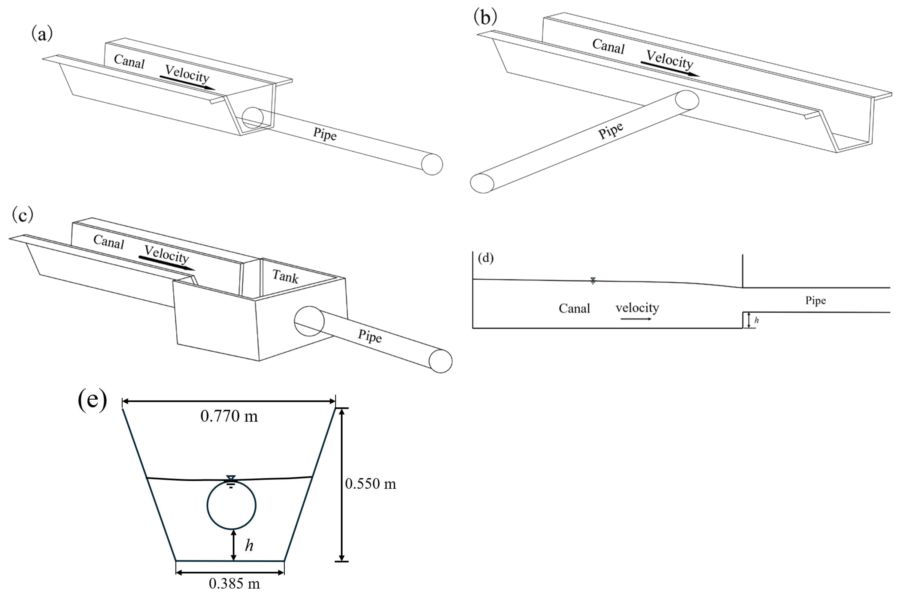Pipe-based water conveyance technology significantly enhances efficiency and optimizes resource utilization, playing a pivotal role in modern agricultural irrigation systems [4]. Recent canal modification projects in several major irrigation districts across China have demonstrated notable improvements in water transport efficiency. Nevertheless, the large-scale deployment of pipe-based water conveyance systems still necessitates substantial financial investment. Considering China’s current economic development level and the state of its irrigation infrastructure, the adoption of a combined canal and pipe water conveyance system (CCPS) has become increasingly imperative. A CCPS uses a canal and pipe to share the water conveyance task, usually with the canal located upstream and the pipe located downstream. According to the connection mode of downstream pipe and upstream canal, a CCPS can be divided into the canal end connection (Figure 1a), the canal sidewall connection (Figure 1b), and the three forms of the canal–tank–pipe connection (Figure 1c). A CCPS effectively integrates the respective advantages of both canal and pipe technologies, significantly reducing infrastructure costs while simultaneously enhancing water resource utilization and conveyance efficiency. To maximize the efficiency of a CCPS, optimizing hydraulic performance at canal–pipe junctions—by mitigating flow disruptions and minimizing energy losses—is crucial. Addressing these technical and economic challenges will be pivotal for facilitating the development and widespread implementation of CCPSs in modern agricultural irrigation systems.

The CCPS encompasses a rich historical development. Japan emerged as a pioneer by implementing CCPSs as early as the 1960s [5]. Following this, in the mid-1980s, the former Soviet Union established formal regulatory frameworks to govern the design and operation of pipe-based irrigation systems, particularly in newly developed agricultural regions. By the late 20th century, the San Joaquin River Valley Irrigation District in California successfully completed the conversion of its branch canals and associated canals into pipe-based systems, showcasing a significant advancement in water conveyance technology [6]. Within the Chinese context, Shi conducted a focused study on the improvements in irrigation water utilization efficiency achieved by replacing traditional canals with pipes at various hierarchical levels. Employing economic benefits as a primary evaluation indicator, his research concluded that canal pipelining below tertiary canals constitutes the optimal model for enhancing irrigation efficiency within the study area [7]. Li et al. [8] conducted an in-depth investigation into the effects of side slopes and diversion angles on local head loss within trapezoidal canals. Their findings revealed a significant negative correlation between local head loss and the relative opening of sectional gates [8]. Gao et al. conducted innovative pipe-based water conveyance experiments within the Yumenkou Irrigation District, establishing a technical model for optimizing pipe arrangements [9]. Gong et al. [10] further demonstrated that implementing a CCPS at the canal terminus in large-scale irrigation districts is both economically viable and technologically feasible for water-saving renovation. Lu’s research highlighted that in hilly canal irrigation districts, replacing terminal canals with pipes led to a nearly 3% reduction in land use [11]. Similarly, Wang reported a significant increase in irrigation water utilization efficiency, with rates rising from 35~60% to approximately 85% following the replacement of terminal canals with pipes [12]. Xie et al. explored the substitution of pipes for terminal canals in the Bayi Irrigation District [13], while Zhang et al. investigated the use of low-pressure pipes for canal replacement in the Yumenkou irrigation district [14,15]. Their findings revealed a 20% improvement in irrigation water utilization efficiency after the canal-to-pipe conversion [14]. Shen et al. analyzed the influence of varying canal water depths on flow velocity distribution within the canal section, pipe diversion ratio, and other parameters when pipes are connected to the canal’s sidewall [16]. Jia et al. [17] extended this research by examining the effects of canal flow velocity distribution and pipe diversion ratio under different pipe depth ratios when the pipe is connected to the sidewall of the canal. Their results indicated that the pipe diversion ratio increased with filling degree under constant canal flow rates [17,18].

Numerical simulation has emerged as a crucial tool for studying the hydraulic performance of structural fluids [19]. By leveraging advanced numerical models, simulations can be conducted under a wide range of working conditions, providing robust support for both research and engineering applications. Ding addressed specific challenges in the water conveyance project of the Pack Ying Reservoir irrigation district, comparing the advantages of pipe-based water conveyance and optimizing the system based on computational results [20]. Lu utilized ANSYS FLUENT (ANSYS Inc, 2013) software to simulate the pattern of lead concentration changes at taps in a copper water supply system; the model incorporated elements such as turbulence dispersion, delivering highly accurate prediction results [21]. Qin et al. explored the gas aggregation law and flow field performance in shale gas-gathering pipes using FLUENT, offering valuable insights into pipe behavior [22]. Xu et al. simulated the process of crude oil displacement water using FLUENT software, and the numerical simulation results were consistent with the experimental results [23]. Wang et al. conducted numerical simulations of a Y-shaped asymmetric confluence canal using FLUENT. Their results demonstrated that the confluence flow behavior can be quantitatively characterized by this model [24]. Muhammad Asif et al. [25] utilized FLUENT software to simulate the flow performance in an asymmetric vegetated composite canal. The simulation results demonstrate that FLUENT can relatively accurately reflect the flow performance and turbulence features of the canal [25]. Sui et al. [26] simulated the flow regimes in a curved bend under different discharge ratios and intersection angles and analyzed the performance of the separation zone. The numerical calculation results are in good agreement with the experimental data [26]. Pritam Kumar et al. simulated the three-dimensional flow of water in a narrow-slit canal using FLUENT, and the simulation results were in general agreement with the experimental observations [27]. In summary, many scholars have carried out a lot of research on the structural flow field using FLUENT, and the numerical calculation results are basically consistent with the experimental results, and the simulation results can reflect the performance of the flow field, which indicates that FLUENT can be used to calculate the flow field distribution law under different working conditions.

In conclusion, extensive research has been conducted on water conveyance through canals and pipe-based irrigation districts, yielding comprehensive findings. However, investigations into the hydraulic performance of CCPSs, particularly those incorporating pipe installation, remain limited, necessitating further exploration. This study aims to provide a detailed analysis of hydraulic performance in CCPSs, elucidating flow field variations at canal–pipe junction points and the distribution performance of the turbulent kinetic energy (TKE) and turbulent eddy dissipation rate (TED). The findings are expected to support the optimal design and safe operation of CCPSs.

2. Materials and Methods

This paper focuses on the connection form that the pipe connects to at the end of the trapezoidal canal (Figure 1a). A combined approach of experimental research and numerical simulations is employed to analyze the impact of pipe installation height on the hydraulic performance of the system. Pipe installation height (H) is defined as the vertical distance from the outer wall of the pipe to the bottom of the canal (Figure 1d).

2.1. Hydraulic Experiment

The experiments were conducted at the National Engineering Research Center for Water-saving Irrigation in Beijing, utilizing a purpose-built experimental platform designed for precise hydraulic performance. The platform, as illustrated in the accompanying schematic, integrates multiple hydraulic components, including a reservoir, a regulated tank, solenoid-controlled valves, flow-stabilizing baffles, a centrifugal pump, a tail pond tank, an electromagnetic flow meter, high-accuracy pressure transducers, and precision water level needles. The pipe installation height is 0.050 m, the canal bottom width is 0.385 m, and the side slope ratio is 0.350 (Figure 1e). The pipe, fabricated from polyvinyl chloride (PVC), was specified with an outer diameter of 160.00 mm and a wall thickness of 4.00 mm. The gradient of both the main canal and the branch pipe is 0.00075. The experimental flow rates were 5.00, 6.25, 9.25, 11.00, and 12.25 L/s, respectively.

Water depth measurements were systematically obtained using calibrated depth gauges (the measuring range is 60 cm and the accuracy is 0.1 mm.) at upstream locations relative to the interface of the CCPS. Downstream hydraulic parameters were monitored using U-tube manometers (Figure 2).

2.2. Numerical Calculations

Numerical calculations were conducted using ANSYS FLUENT (the software is licensed for ANSYS 2020).

2.2.1. Governing Equations

The governing equation commonly used here for incompressible viscous liquids is as follows:

Continuity equation, momentum equation, and turbulence; RNG $k-\epsilon$ model. Other scholars used the RNG $k-\epsilon$ model to simulate the water flow movement [28,29]. In this study, since the water flowed from the canal into the pipe, the cross-sectional area of the flow decreased sharply, causing the flow pattern in the flow field to become disordered. Therefore, this turbulent flow model was selected for calculation. The momentum balance by Navier–Stokes equation considers the Reynolds averaging, i.e., ${\Phi }_i={\overline{\Phi }}_i+{\Phi }_i^{\prime }$, where ${\overline{\Phi }}_i$ and ${\Phi }_i^{\prime }$ are the mean and fluctuating components of flow properties, respectively. Therefore, the instantaneous conservation equations with time-averaging become ensemble average equations. Using Cartesian tensor notation, the continuity and momentum equations can be written as follows:

Continuity equation:

$${\displaystyle \frac{\partial \overline{u}}{\partial x_i}}=0$$

(1)

$${\displaystyle \frac{\partial }{\partial x_j}}(\rho \overline{u_i{u}_j})=-{\displaystyle \frac{\partial \overline{p}}{\partial x_i}}+{\displaystyle \frac{\partial }{\partial x_j}}(\mu {\displaystyle \frac{\partial \overline{u_i}}{\partial x_j}})-{\displaystyle \frac{\partial }{\partial x_j}}(\rho \overline{{u^{\prime }}_i{u^{\prime }}_j})$$

(2)

where p means pressure (pa); $\rho$ is the fluid material density; $\overline{u_i}$ is the time-averaged velocity component (m/s); $\rho \overline{u_i{u}_j}$ is the Reynolds stress; and x_i and x_j are coordinate vectors (i, j = 1, 2, 3).

Solving such a system of equations allows the velocity and pressure to be evaluated at each model section for geometry of varying complexity. Both numerical environments used provide the ability to consider laminar and turbulent flows for compressible fluids using the RANS model. This approach makes it possible to implement RNG $k-\epsilon$ and evaluate the effect of turbulence on the flow parameters after finding the 4t values from the kinetic energy of the vortices, k, and the dispersion rate, E.

$${\displaystyle \frac{\partial (\rho k)}{\partial t}}+{\displaystyle \frac{\partial (\rho k{u}_i)}{\partial x_i}}={\displaystyle \frac{\partial }{\partial x_j}}\left[{\alpha }_k{\mu }_{\mathrm{eff}}{\displaystyle \frac{\partial \epsilon }{\partial x_j}}\right]+G_k+\rho \epsilon$$

(3)

$${\displaystyle \frac{\partial (\rho \epsilon )}{\partial t}}+{\displaystyle \frac{\partial (\rho \epsilon u_i)}{\partial x_i}}={\displaystyle \frac{\partial }{\partial x_i}}\left[{\alpha }_{\epsilon }{\mu }_{\mathrm{eff}}{\displaystyle \frac{\partial \epsilon }{\partial x_j}}\right]+{\displaystyle \frac{C_{1\epsilon }}{k}}{G}_k+C_{2\epsilon }\rho {\displaystyle \frac{{\epsilon }^2}{k}}$$

(4)

where $\mu$ is the hydrodynamic viscosity coefficient (${\mu }_{\mathrm{eff}}=\mu +{\mu }_t$, N·s/m²); ${\mu }_t$ is the fluid vortex viscosity (N·s/m²); G_k is a TKE production term due to the mean velocity gradient (m²/s²); ${\alpha }_k$ and ${\alpha }_{\epsilon }$ are the inverse of the effective Prandtl numbers of k and ε, respectively—${\alpha }_k={\alpha }_{\epsilon }=1.39$; and C_1ε, C_2ε are model constants whose values are determined experimentally—$C_{1\epsilon }$ = 1.42, $C_{2\epsilon }$ = 1.68.

2.2.2. Boundary Conditions

Numerical calculation of the boundary conditions and solution methods are as follows: the upstream canal inlet boundary conditions are set as mass flow inlet, and the corresponding mass flow rate value is given; the outlet boundary conditions are pressure outlet, and the boundary conditions in the upper part of the canal are free boundary with free air access. To consider the influence of air on the flow velocity, the free surface treatment abandons the ‘rigid cover’ assumption commonly used in open canal uniform flow simulation, and the Volume of Fluid (VOF) method is adopted. VOF is a common technique for tracking the interface of two-phase flow in computational fluid dynamics (CFD) simulation. In the VOF method, a function is defined to track the volume fraction of the fluid, which is essential for simulating multiphase flow. This function ranges from 0 to 1, where a value of 0 indicates the absence of liquid in a grid cell and a value of 1 signifies that the grid cell is entirely filled with water. Interface capture is critical during VOF simulations, which can accurately track the change in the free surface of the water flow [30]. The wall boundary condition is a no-slip solid wall condition, where the wall roughness is quantified by setting the average roughness layer height k_s of the wall particles, and the flow velocity distribution in the vicinity of the wall is determined by the scalable wall function.

The momentum and energy equations are solved using the Second Order upwind scheme while the geometric reconstruction method is used to solve the volume fraction equation. The surface tension is converted to volume force through the CSF (Continuum Surface Force) model while the Pressure-Implicit with Splitting of Operators (PISO) algorithm is used to couple pressure and velocity fields [31]. The value of the computational residuals is set to 10⁻⁴. In addition, transient simulations are performed through a variable time-stepping strategy using the courant number.

2.2.3. Meshing

The numerical computational model is constructed based on the experiment, and the numerical model has the same dimensions as the experiment. Unstructured grids were used to perform the mesh dissections across the entire computational threshold (according to Figure 3), and the numerical solutions obtained from different grid sizes were compared with those obtained from the hydraulic experiment (Figure 4).

A grid independence analysis was performed to ensure that the numerical results were not affected by the grid resolution. Local head loss is an important indicator of the rationality of the structure [32,33]. The formula is:

$$h_w=E_1-E_2=({\displaystyle \frac{{\overline{V_1}}^2}{2g}}-{\displaystyle \frac{{\overline{V_2}}^2}{2g}}-{\displaystyle \frac{P_2}{\rho g}})+Z_1-Z_2$$

(5)

where $h_w$ is the local head loss (m). According to Figure 4, E₁ and E₂ are the upstream (B-B’) and downstream (F − F’) energy values (m), respectively. ${\overline{V}}_1$ and $\overline{V_2}$ are the average flow velocities at the upstream and downstream sections (m/s), respectively. Z₁ and Z₂ are the upstream and downstream section location heads. During the calculation process, the water depth and cross-sectional average flow velocity at a position 0.30 m upstream of the canal–pipe junction are selected, while the water depth and pressure at a position 1.50 m downstream of the junction are chosen as the calculation points for pipe energy. Based on the cross-sectional calculation results, the local head losses under different pipe installation heights and flow rates are computed.

The local head loss values of the CCPS were obtained through experiments, and the relative error values between the simulated and measured values were calculated for different grid numbers. The formula is as follows:

$$\delta ={\displaystyle \frac{\left|h_{w\mathrm{s}}-h_{w\mathrm{e}}\right|}{h_{w\mathrm{s}}}}\times 100\%$$

(6)

where h_ws and h_we are numerically simulated and experimentally observed local head loss values, respectively.

The relative error between the simulated and measured values of water depth in the combined canal and pipe conveyance system is calculated in the following equation:

$$\delta ={\displaystyle \frac{1}{n}}{\displaystyle \sum _{i=1}^n\frac{\left|h_{\mathrm{s}i}-h_{\mathrm{r}i}\right|}{h_{\mathrm{r}i}}}$$

(7)

where h_si is the simulated value of water depth in cm; h_ri is the measured value of water depth in cm; and n is the number of measurement points.

2.2.4. Numerical Simulation Scheme

Numerical simulation sets two variables, pipe installation height and flow rate. The pipe installation heights were 0, 1, 3, and 5 cm, for a total of four levels. Six flow rates, 18.40, 21.21, 24.74, 28.27, 33.58, and 38.88 L/s (the water flow velocity was selected between 1.0 and 2.2 m/s.), were determined based on the actual water delivery and the economic flow rate of the pipe.

To investigate the influence of pipe installation heights on the hydraulic performance of the CCPS under varying flow rates, six cross-sections were selected for analysis: P0 (A − A’) at 0.48 m, P1 (B − B’) at 0.32 m, P2 (C − C’) at 0.16 m, and P3 (D − D’) at 0.08 m upstream of the canal–pipe junction, as well as P4 (E − E’) at 0.80 m and P5 (F − F’) at 1.60 m downstream.

2.3. Hydraulic Performance Indicators

2.3.1. Local Head Loss Calculation Method

Localized head loss is a key indicator of the merits of the design of CCPSs, and its calculation equation is shown in (5).

2.3.2. TKE Calculation Method

TKE is a very important characterization index for describing the intensity of fluid turbulence. The calculation method depends on the velocity component fluctuations of the turbulence. In a three-dimensional flow field, the formula for calculating TKE is as follows:

$$\mathrm{TKE}={\displaystyle \frac{1}{2}}(u^{\prime 2}+v^{\prime 2}+w^{\prime 2})$$

(8)

where $u^{\prime 2}$, $u^{\prime 2}$ and $u^{\prime 2}$ represent the fluctuating velocity components of the fluid in the x, y, and z directions, respectively. The fluctuating velocity components $u^{\prime 2}$, $v^{\prime 2}$, and $w^{\prime 2}$ refer to the deviations of the fluid velocity from its average value, calculated by Equations (9)–(11):

$$u^{\prime }=u-〈u〉$$

(9)

$$v^{\prime }=v-〈v〉$$

(10)

$$w^{\prime }=w-〈w〉$$

(11)

where $〈u〉$, $〈v〉$, $〈w〉$ represent the time-averaged flow velocities of the fluid in the x, y, and z directions, respectively.

2.3.3. TED Calculation Method

TED is a physical quantity that describes the rate at which TKE is converted into heat or dissipated, reflecting the attenuation process of the total velocity fluctuations in turbulence. Its calculation method is as follows (12):

$$\epsilon =v{\displaystyle \frac{\partial u_i^{\prime }}{\partial x_j}}{\displaystyle \frac{\partial u_i^{\prime }}{\partial x_j}}$$

(12)

where $v$ is the kinematic viscosity of the fluid and $u_i^{\prime }$, i, and j are the velocity components in the i and j direction in the spatial coordinates.

2.3.4. The Uniformity of the Flow Velocity Distribution Calculation Method

The uniformity of the flow velocity distribution is determined according to (13):

$$V_u=\left[1-{\displaystyle \frac{1}{\overline{u_a}}}\sqrt{{\displaystyle \frac{\sum {\left(u_i-{\overline{u}}_a\right)}^2}{m}}}\right]$$

(13)

where V_u is the uniformity of flow velocity distribution; u_a is the cross-section mean flow rate; u_i is the flow rate at the ith measurement point; and m is the number of flow measurement points in the cross section.

3. Results

In this study, hydraulic parameters such as water depth, local head loss, cross-sectional flow velocity distribution, TKE, and TED distribution were analyzed.

3.1. Model Verification

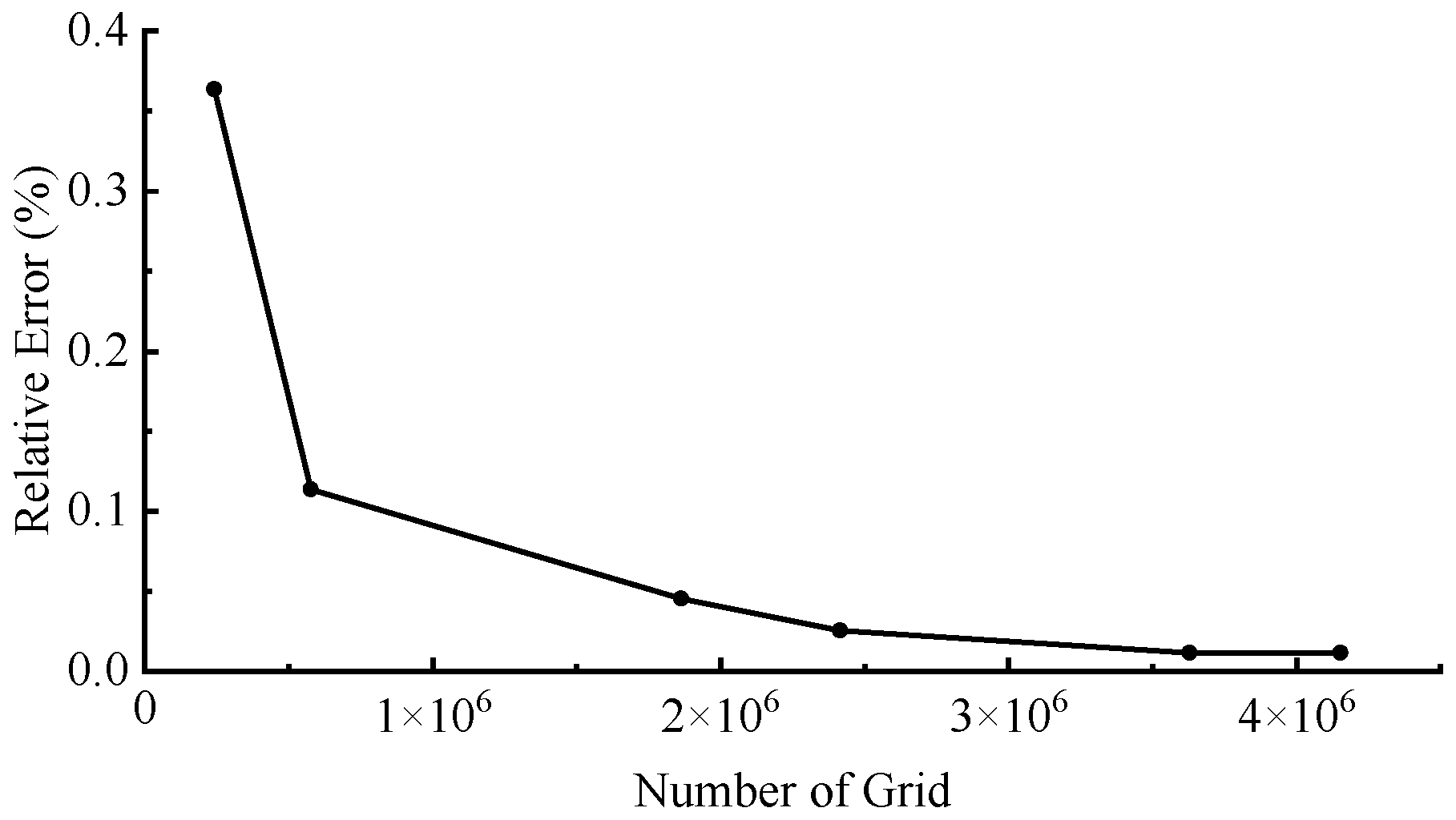
Figure 5 shows the relative error of local head loss under different grid numbers. The relative error of local head loss gradually decreases as the number of grids increases. When the grid count reaches 3.63 million, the relative error approaches the actual value. As the grid number further increases, the rate of error reduction diminishes (Figure 4), demonstrating that the local head loss is directly influenced by the grid configuration. This trend confirms that the current grid scale and numerical model are suitable for CCPS calculations. Balancing computational accuracy and efficiency, the optimal grid number is determined to be 3.63 million.

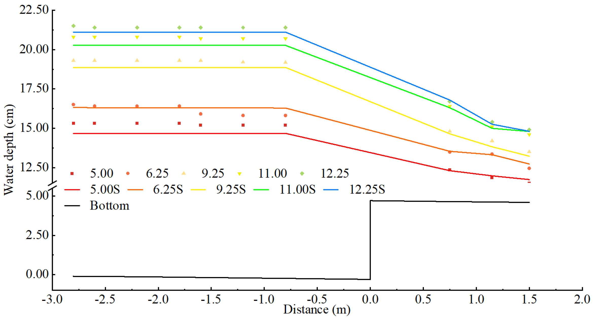
Figure 6 shows the water depth changes with respect to experiment and simulation along the distance. The water depths in both the canal and the pipe, as predicted by the numerical simulations, closely match the experimental data across all flow rates. Upstream of the canal and pipe junction, the canal water depth remains nearly parallel to the canal bottom. As the flow approaches the junction, the canal water depth steepens as it enters the pipe. For flow rates of 5.00 L/s and 6.35 L/s, both the canal’s inflow and the water depth in the pipe decrease slowly. However, at higher rates of 9.25 L/s, 11.00 L/s, and 12.25 L/s, the rate of water depth drops in both the canal and pipe increase noticeably. In this way, the reliability of the numerical model is validated. The average error value between the simulated and measured values of water depth was calculated according to Equation (7). According to the flow rate, the average value of the relative error of water depth at each flow rate was 3.03%, 1.61%, 2.08%, 19.4%, and 1.12%. The experimental data agree well with the calculated results, showing consistent trends in water depth, which confirms that the numerical results are reasonable and reliable.

3.2. Water Depth

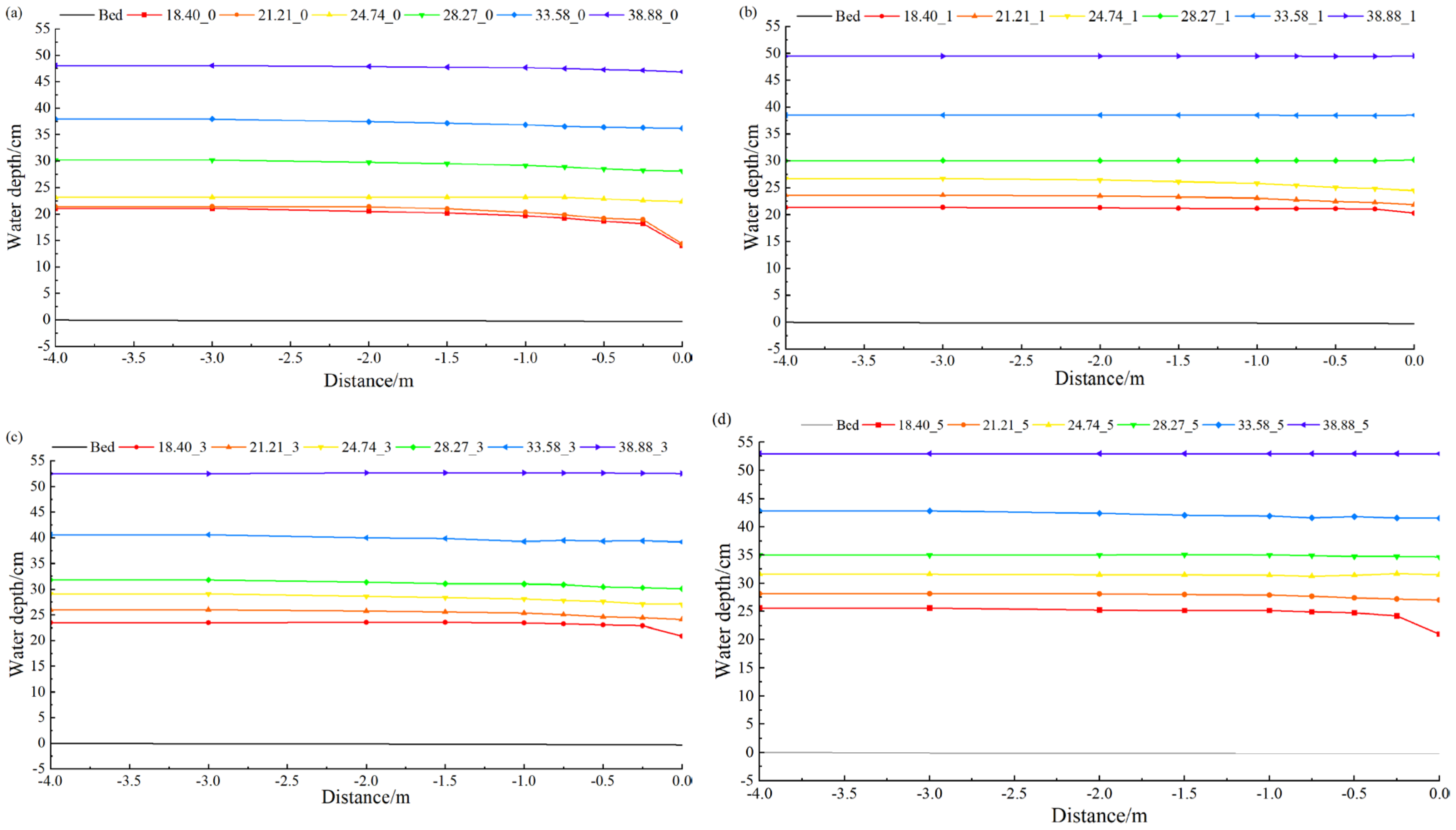
Figure 7 shows the simulated canal water depth variations along the canal under different pipe installation heights and flow rates. The water depth in the canal increases gradually with the height of the pipe installation and the flow rate. Away from the junction between the canal and the pipe, the canal water depth gradually increases with the installation height and flow rate of the pipe, and the canal water surface line is basically parallel to the bottom of the canal. When the flow rate is lower than 21.21 L/s, the water depth of the canal varies little at the four pipe installation heights. However, when the flow rate exceeds 21.21 L/s, the water depth of the canal varies more significantly at the four pipe installation heights. Close to the junction of the canal and the pipe, the water depth in the canal increases gradually with the installation height and flow rate of the pipe. However, the trend of the free surface of the canal varies under different installation heights and flow rates. When the pipe installation height is constant and the flow rate is small, the canal water depth at the junction decreases steeply. As the flow rate increases, the drop rate of water depth at the junction decreases. When the flow rate gradually increases, the water depth at the junction is congested. When the flow rate is lower than 28.27 L/s, the coupling effect of pipe installation height and flow rate causes the canal water depth to appear to be higher at adjacent flow rates for larger flow rates and smaller pipe installation heights than for smaller flow rates and larger pipe installation heights.

In the area where the canal and pipe are combined and connected, the cross section of water flow in the canal is large, but it becomes smaller after the water enters the pipe, leading to a steep decrease in the cross section at the canal–pipe junction, which causes an increase in the canal water depth. As the installation height of the pipe gradually increases, the canal water depth also rises to facilitate water flow into the pipe. This occurs because the lower part of the pipe increasingly impedes the water flow, resulting in a gradual increase in the canal water depth. At lower flow rates, the water surface profile drops steeply at the point where the pipe meets the canal, and the water flows freely into the pipe. However, as the pipe installation height increases, for the same flow rate, canal water depth rise leads to a decrease in the average velocity through the canal, which requires additional potential energy, thus causing the water surface profile to gradually increase.

3.3. Local Head Loss

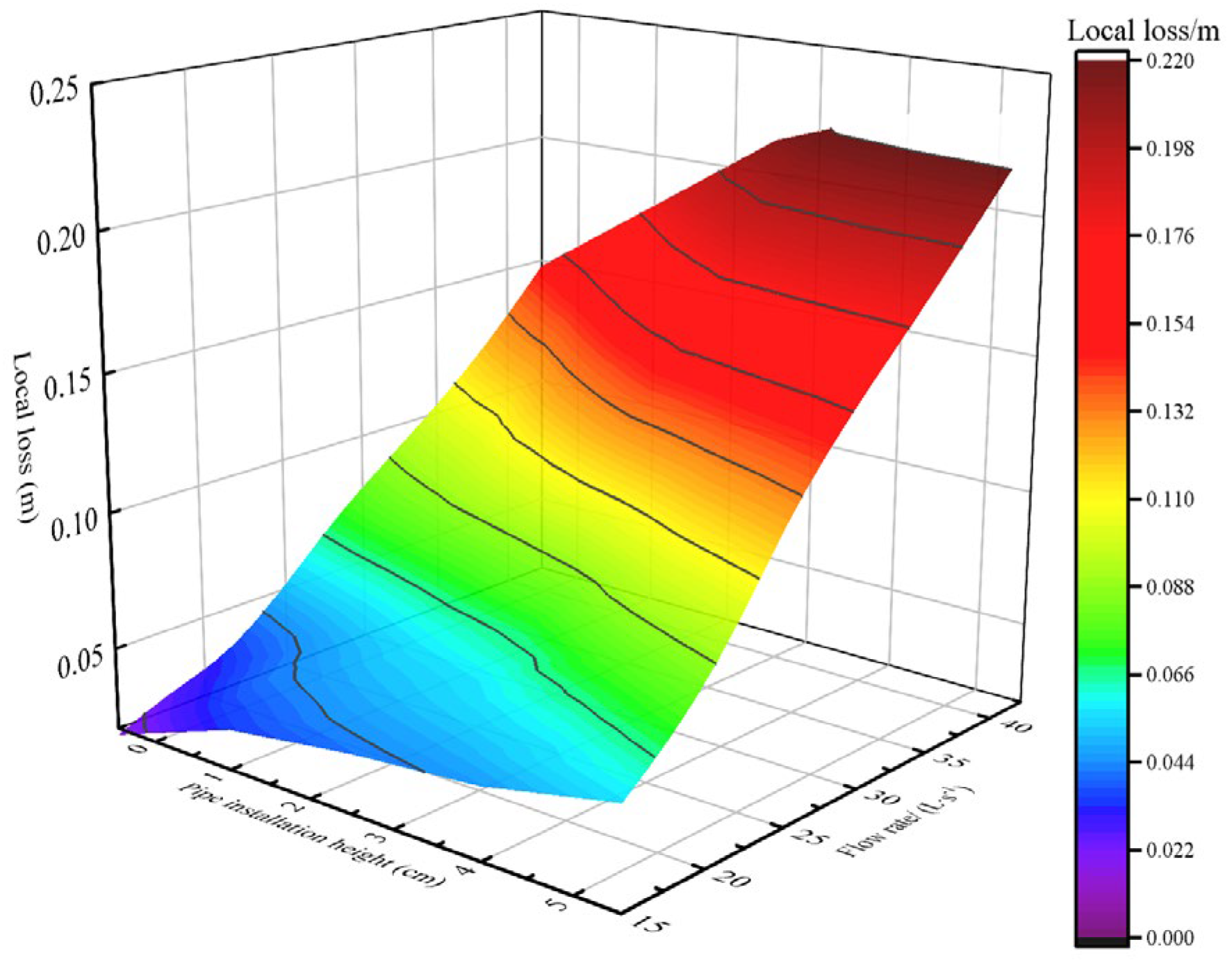
Figure 8 shows the contour of local head loss under varying pipe installation heights and flow rates. Overall, the local head loss increases gradually with pipe installation height and flow rate. For a given flow rate, the local head loss increases gradually with higher pipe installation heights. The local head loss at each pipe installation height shows a quadratic parabolic distribution with the increase in flow rate, with R² between 0.982 and 0.991 (

Table 1. Expression for variation in water depth with flow rate at different pipe installation heights.

Pipe Installation Height/cm	Expression	R2
0	$H=0.0419\times Q^2-0.9532\times Q+20.981$	0.9976
1	$H=0.0487\times Q^2-1.3870\times Q+29.9080$	0.9990
3	$H=0.0634\times Q^2-2.2121\times Q+42.514$	0.9988
5	$H=0.0307\times Q^2-0.4073\times Q+21.8630$	0.9938

). The increase in local head loss at different pipe installation heights in different flow ranges is not the same. When the flow rate is between 18.40 and 24.74 L/s, the local head loss at the installation heights of 0 cm, 1 cm, and 3 cm is relatively small, and it is significantly different from that at 5 cm. As the flow rate continues to increase, the local head loss at 3 cm gradually becomes larger than that at 0 cm and 1 cm. However, the difference in local head loss between 3 cm and 5 cm gradually decreases. This is because when the flow rate is small, the canal water depth and flow velocity at installation heights of 0, 1, and 3 cm vary little, and the local head loss is close. However, at 5 cm, due to the large water depth, when the water flows to the connection point, due to the obstruction effect of the interface, a large energy loss occurs. As the flow rate increases, the water depth difference at 3 and 5 cm gradually decreases. Currently, the difference in local head loss at the two installation heights gradually declines (

Table 2. Expression for variation in local head loss with flow rate at different pipe installation heights.

Height/cm	Expression	R2
0	$h_{\mathrm{w}}=8E-05\times Q^2+0.0117\times Q-0.1227$	0.989
1	$h_{\mathrm{w}}=0.0002\times Q^2-0.0041\times Q+0.0623$	0.991
3	$h_{\mathrm{w}}=0.0001\times Q^2+0.0014\times Q-0.0167$	0.982
5	$h_{\mathrm{w}}=0.0071\times Q-0.0598$	0.991
0/1/3/5	$h_{\mathrm{w}}=6.2054E-05\times Q^2-0.0005\times H^2+0.0005\times Q\times H+0.0018\times Q+0.0019\times H-0.0265$	0.978

h_w is the local head loss, Q is the flow rate in L/s, and H is the pipe installation height in cm.

).

The increase in pipe installation height requires a higher water depth due to the sharp reduction in junction area, which restricts water exchange between the canal and pipe, thereby gradually reducing the interfacial flow rate. Compared to pipes installed at lower heights, those placed higher need greater water depths to maintain flow, leading to progressively higher head losses. As the overall flow rate increases, the rising velocity in the overflow section amplifies local head losses since these losses are intrinsically tied to flow velocity. However, at low flow rates, minimal variations occur in both canal water depth and flow distribution across different installation heights, resulting in negligible differences in local head loss.

3.4. Velocity Distribution

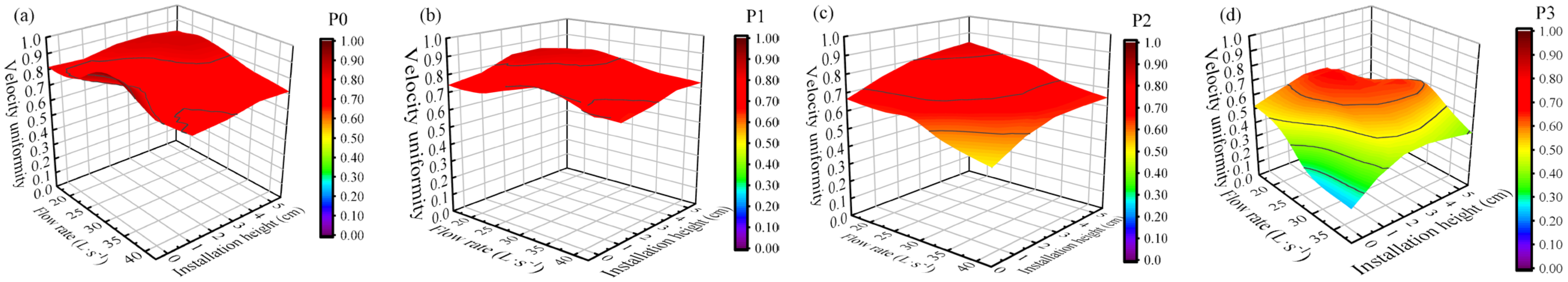
Figure 9 shows the contours of velocity uniformity distribution across different canal cross-sections under varying pipe installation heights and flow rates. P0, P1, P2, and P3 are typical sections of the canal (Figure 6). As the distance between the observed cross-section and the junction point increases, the uniformity of the flow velocity distribution in the cross-section gradually increases. Under different flow rates, the difference in the uniformity of flow velocity at sections P1, P2, and P3 is large, the difference in the uniformity of flow velocity distribution at sections P0 and P1 is small, and the trend is basically the same under each flow rate. Taking 18.40 L/s as an example, the flow velocity uniformity increased by 20% (0 cm) to 90% (5 cm) in section P2 compared to P3, 1.22% (5 cm) to 10.61% (0 cm) in section P1 compared to section P2, and 1.23% (5 cm) to 6.85% (0 cm) in section P0 compared to section P1. The results show that when the installation height is low, the disturbance range is wider due to the greater influence of the CCPS on the flow velocity distribution in the upstream canal, and the disturbance of the canal flow by the CCPS is effectively reduced by increasing the installation height of the pipe. Moreover, the difference between the uniformity of flow velocity distribution in cross-section P1 and section P0 is small, and this section can be regarded as the furthest section affected by the CCPS. P3 is the section nearest to the junction point of the canal pipe, and the trend of different pipe installation heights varies with the increase in flow rate. When the installation height of the pipe is 0, 1, and 3 cm, the uniformity of cross-sectional flow velocity distribution shows a gradual decrease with the increase in flow rate, and the uniformity of cross-sectional flow velocity under each flow rate increases gradually with the increase in the installation height of the pipe. Unlike the other three pipe installation heights (P3), when the pipe installation height is 5 cm, the uniformity of cross-sectional flow velocity distribution changes with the increase in flow rate in a ‘∧’ type. Under the same flow rate, the uniformity of cross-sectional flow velocity distribution and the installation height of the pipe show a ‘∧’ type trend. When the flow rate is 18.40~24.74 L/s, the difference in cross-sectional flow velocity distribution uniformity is small under four pipe installation heights. When the flow rate is 28.27~38.88 L/s, the difference in cross-sectional flow rate distribution uniformity is small when the installation height of the pipe is 0 cm, and with the increase in flow rate and installation height of the pipe, the difference in cross-sectional flow rate uniformity gradually increases.

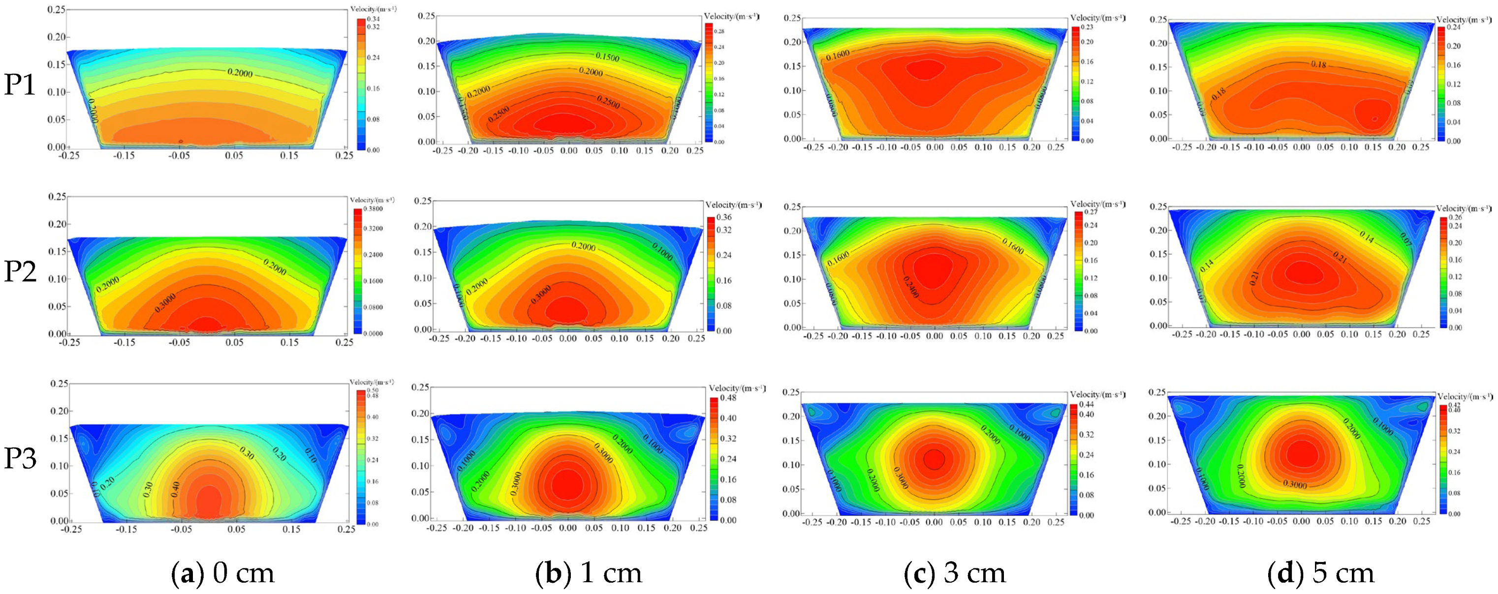
Figure 10 shows the distribution of flow velocity across the canal cross-section at different positions and pipe installation heights. The cross-sectional flow velocity distribution remains consistent across different flow rates. This section takes a flow rate of 18.40 L/s as an example to analyze the influence of pipe installation height on the cross-sectional flow velocity distribution. In the same canal section, as the pipe installation height increases, the distribution area of higher flow velocity values gradually shifts upward, and the maximum flow velocity value gradually decreases. At the same installation height, as the distance between the section and the connection point decreases, the distribution area of higher flow velocity values gradually narrows, the maximum flow velocity value gradually increases, and the variation in the cross-sectional flow velocity distribution becomes more pronounced.

The increase in pipe installation height leads to an increase in canal water depth and a decrease in cross-sectional average flow velocity. When the pipe installation height increases, the mainstream area of the canal water flow gradually moves upward, essentially appearing directly in front of the pipe. Compared with a low pipe installation height, the increase in pipe installation height has a rectification effect on the canal water flow. In the three sections upstream of the connection point, the difference in the flow velocity distribution across the three sections due to the pipe installation height structure is minimal.

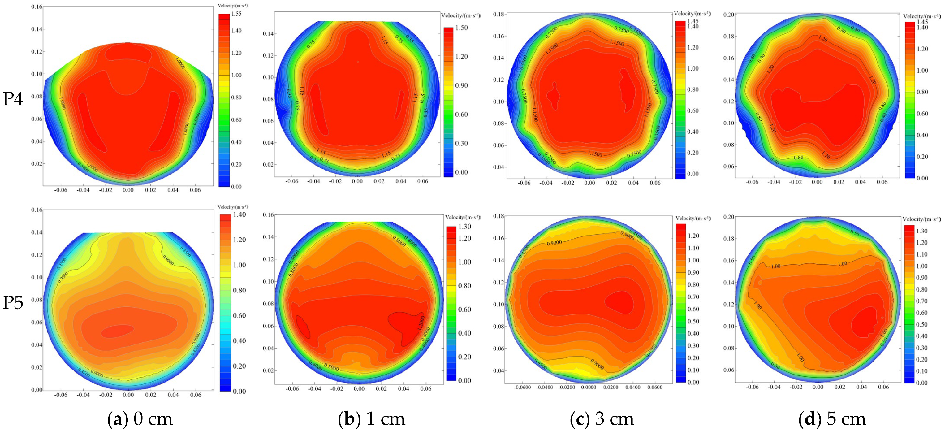
Figure 11 shows the velocity distribution across pipe cross-sections at various positions under different installation heights. As the pipe installation height increases, the flow transitions from open canal flow to full pipe flow. In section P4, the maximum velocity within the pipe cross-section gradually decreases with increasing pipe installation height, though the maximum velocities remain consistent for installation heights of 3 cm and 5 cm. In section P5, higher flow velocities are predominantly found in the lower region of the cross-section, and the maximum cross-sectional flow velocity tends to decrease as the pipe installation height increases.

The installation height of the pipe significantly influences the state of water flow within it. At the same flow rate, elevating the pipe installation height increases the water depth inside the pipe. This occurs because raising the pipe reduces the average flow velocity across the canal cross-section, consequently increasing the water depth within the pipe. Additionally, the increase in canal water depth and the reduction in average flow velocity result in a smoother water flow into the pipe, leading to a more uniform flow distribution across the pipe cross-section.

3.5. TKE

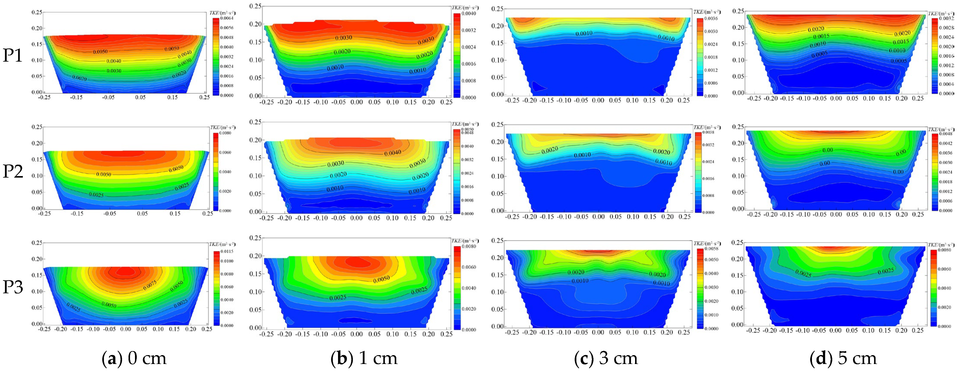
Figure 12 shows the contour of TKE distribution at different canal cross-sections under different pipe installation heights. This section takes a flow rate of 18.40 L/s as an example to analyze the influence of pipe installation height on the cross-sectional TKE distribution. The larger values (the larger value is 80% of the maximum value of the indicator at the corresponding section; this is consistent throughout the text) of TKE TKE are distributed in the lower region of the free liquid surface, and the closer to the canal wall and the bottom of the canal, the smaller the value of TKE. At the same pipe installation height, the maximum value of TKE in the cross-section gradually increases as the distance from the connection point with the canal pipe decreases, and the TKE is more unevenly distributed in the cross-section. At position P1, the maximum value of TKE decreases with the increase in the pipe installation height, and with the decrease in the distance from the connection point with the canal pipe, the maximum value of TKE shows an increase and then a decrease with the pipe installation height. The cross-section TKE is minimized when the pipe installation height is 3 cm, and the maximum value of TKE increases by 42% when the pipe installation height is 5 cm compared to 3 cm. At the P3 position, with the gradual increase in the pipe installation height, the TKE maximum value region gradually moves upward. When the pipe installation height is 0 and 1 cm, the TKE maximum value is distributed in the lower region of the free liquid surface. When the pipe installation height is increased to 3 and 5 cm, the TKE maximum value is distributed in the region of the free liquid surface and the distribution region of the larger value of TKE decreases and concentrates in the position of the free surface.

After the installation height of the pipe increases, the water depth of the canal gradually increases, the average flow velocity in the canal decreases, the water flow fluctuation in the canal is small, and the TKE of the cross-section gradually decreases. As the distance between the section location and the connection point of the canal pipe decreases, the sectional flow velocity distribution changes abruptly due to the reduction in the overflow section, resulting in the concentration of the TKE section region and its gradually increasing.

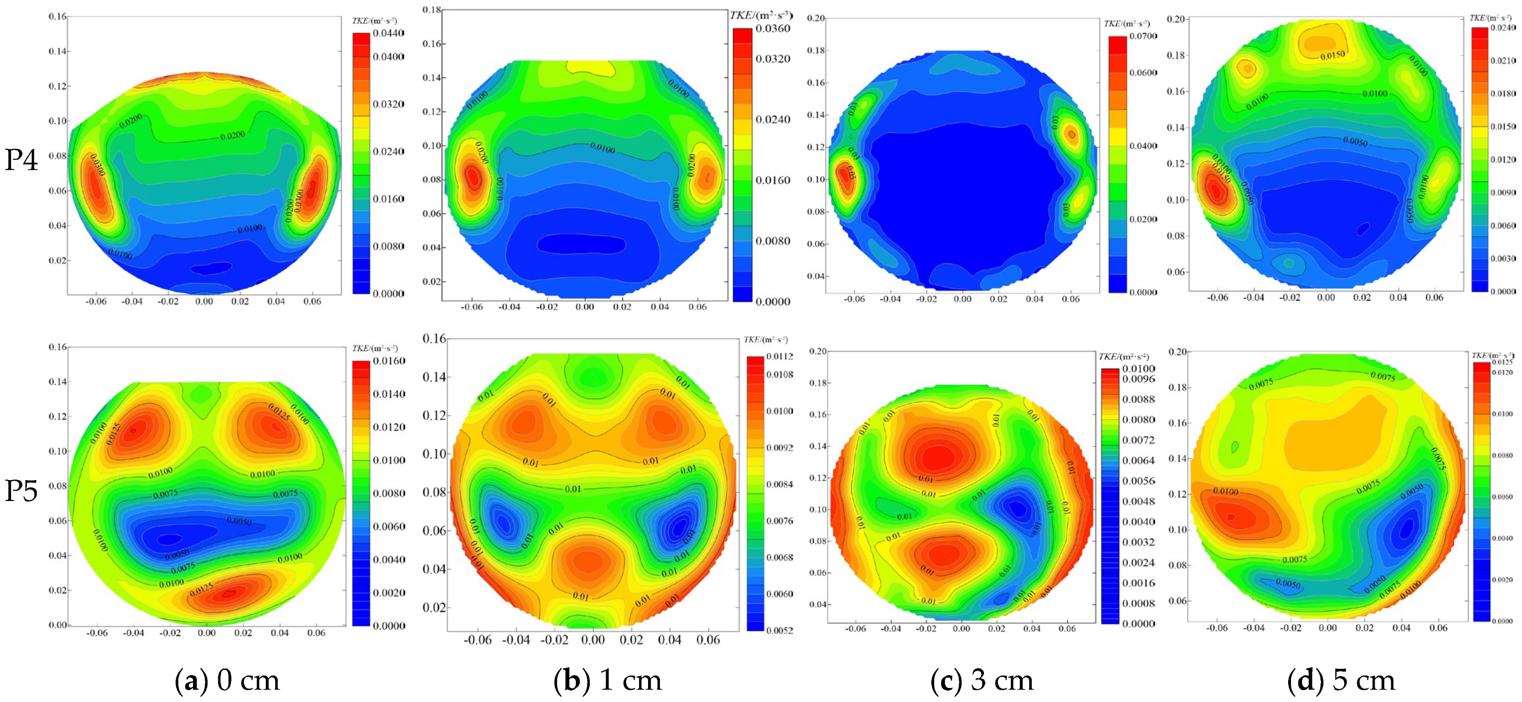
Figure 13 shows the contour of TKE distribution at different pipe cross-sections under different pipe installation heights. At position P4, TKE distribution exhibits similar trends for pipe installation heights of 0 cm, 1 cm, and 5 cm, with higher TKE values primarily concentrated in the lower and upper regions of the pipe wall, while the maximum cross-sectional TKE gradually decreases as the installation height increases. However, a distinct pattern emerges at the 3 cm installation height, where elevated TKE values are distributed along the inner wall of the pipe. Moving to position P5, the cross-sectional TKE demonstrates a non-linear relationship with the installation height, initially decreasing and subsequently increasing as the height rises. This behavior is closely linked to a transition in flow regime: as the installation height increases, the liquid level within the pipe gradually rises and eventually fills the pipe completely, shifting the flow from an open-canal to a full-pipe condition. The intensified TKE observed along both sides of the inner pipe wall is attributed to the reduction in the overflow cross-section, which causes significant flow rate fluctuations along the inner wall as water enters the pipe, thereby elevating TKE values. Notably, at the 3 cm installation height, this effect is particularly pronounced, with higher TKE locally along the lateral walls of the pipe. This phenomenon likely results from the combined effects of reduced overflow in the cross-section and increased flow instability, which amplify turbulence generation in these regions.

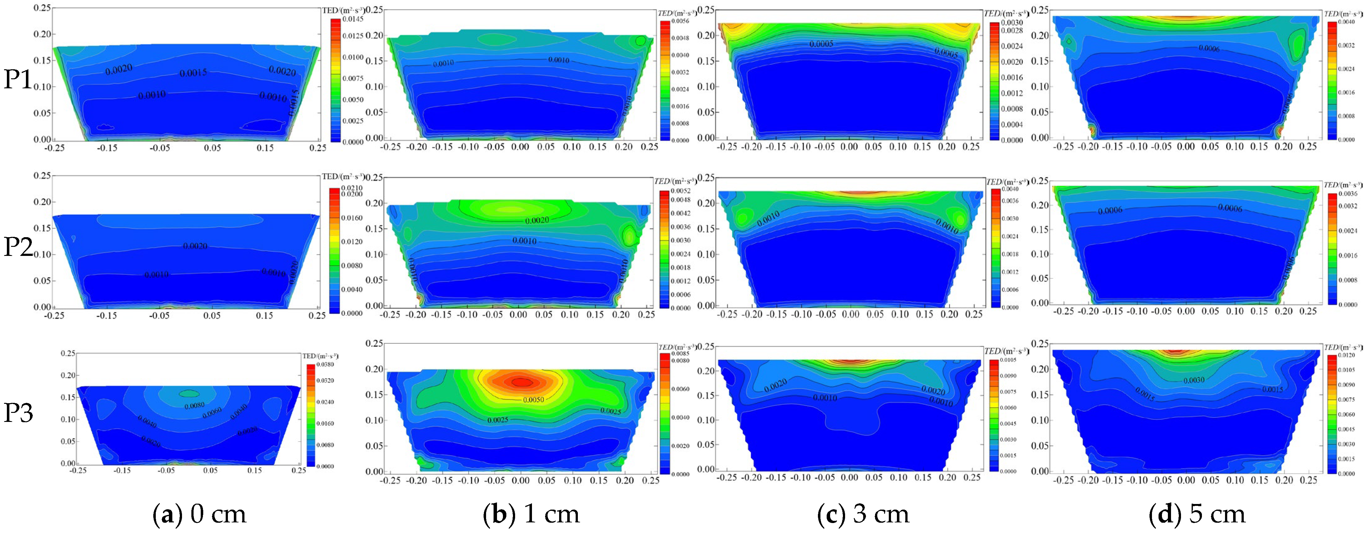
3.6. Turbulent Eddy Dissipation

Figure 14 shows the contour of turbulent eddy dissipation rate distribution at different canal cross-sections under different pipe installation heights. The trend of turbulent eddy dissipation rate distribution in the canal section varies under different pipe installation heights. Increased pipe installation height reduces the maximum turbulent eddy dissipation rate in the cross-section. At a pipe installation height of 0 cm, the larger values of turbulence eddy dissipation rate were distributed at the edge wall and bottom of the canal at P1, and the largest turbulence eddy dissipation rate was at the bottom of the lower part of the pipe. At position P2, the larger values of the turbulent dissipation rate are distributed at the bottom of the pipe, and at position P3, the larger values of the turbulent eddy dissipation rate are found at the bottom of the pipe and at the upper surface region of the pipe. When the installation height of the pipe is 1, 3, and 5 cm, the larger values of the turbulent eddy dissipation rate are distributed in the free surface region at the three positions, and as the installation height of the pipe increases, the distribution region of the larger values of the turbulent dissipation rate decreases gradually and is concentrated in the free liquid surface region at the upper part of the pipe opening.

When the pipe installation height is 0 cm, the canal water depth is relatively shallow, resulting in a higher cross-sectional flow velocity. Under these conditions, the turbulent dissipation rate is predominantly concentrated in the bottom region of the canal. As the installation height of the pipe increases, the fluctuation of the canal water flow at the free liquid surface becomes more pronounced, particularly near the pipe inlet. At lower pipe installation heights, the canal water depth remains limited, leading to a non-full pipe flow regime. Consequently, the turbulence dissipation rate is significantly elevated in the region immediately upstream of the pipe inlet. With further increases in the pipe installation height, the canal water depth rises, transitioning the flow into a full pipe regime. This shift is accompanied by a gradual reduction in the spatial distribution of the turbulent dissipation rate, with the dissipation becoming more localized in specific areas.

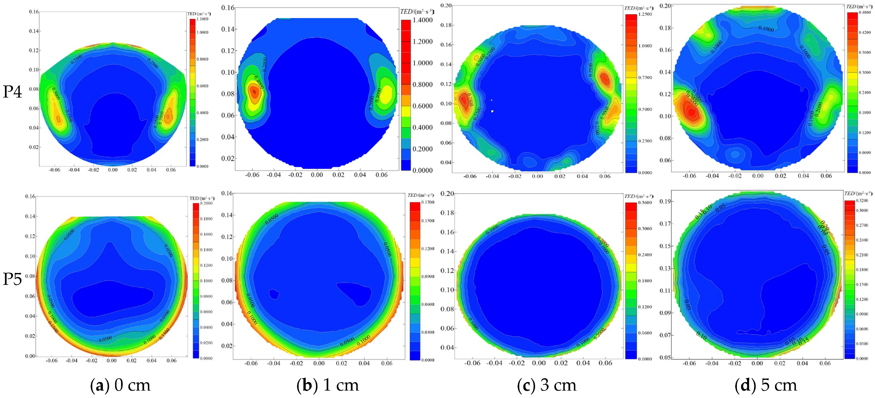
Figure 15 shows the contour of the turbulent dissipation eddy rate at the pipe cross-section under varying pipe installation heights. In section P4, the higher values of the turbulent dissipation rate are primarily local along the inner wall of the pipe, particularly on both sides of the section. The maximum turbulent dissipation rate at this section exhibits a gradual decline as the pipe installation height increases. In section P5, the turbulent dissipation rate is predominantly distributed along the pipe wall, with the larger values concentrated in the middle and lower regions of the wall. Across the four tested pipe installation heights, the turbulent dissipation rate reaches its minimum at 1 cm and peaks at 5 cm. Notably, at the P5 position, the turbulent dissipation rate is significantly lower compared to the P4 position for all installation heights. However, it demonstrates a trend of initially decreasing and then increasing as the pipe installation height rises, with the lowest value observed at 1 cm and the highest at 3 cm.

4. Discussion

The impacts of different flow rates and pipe installation heights on canal water depth, local head loss, and uniformity of cross-sectional flow velocity, as well as TKE and turbulent dissipation eddy rate distribution, were previously described. The above indicators affect the project scale, investment, distribution of hydraulic properties, etc., and the trend of each indicator varies with the height of pipes installed.

Canal water depth is a key element that affects canal size, project investment, and operation and maintenance, and canal water depth is positively correlated with project investment. Canal water depth shows a gradual increase with the increase in pipe installation height and flow rate, but there are obvious differences in the performance trend under different combinations of flow rate and pipe installation height. The free surface is higher in the small flow and high installation height case than in the large flow and small installation height case. Observing the canal water depth at 2 m upstream of the junction point, the canal water depth and flow rate under four pipe installation heights showed a second polynomial distribution, with R² between 0.994 and 0.997. Differences in canal water depth between installation heights of 0, 1, and 3 cm diminished as flow rate increased. The variation in water depth caused by the change in pipe installation height is larger than that caused by the change in flow rate.; e.g., channel water depths were higher at a flow rate of 18.40 L/s and an installation height of 1 cm than at a flow rate of 21.21 L/s and a pipe installation height of 0 cm. Canal water depth affects the height of the canal, which further affects the project scale and investment cost. Therefore, under the same flow, the smaller the channel water depth, the better the project scheme.

Local head loss is an important parameter to measure the design advantages and disadvantages of CCPSs. As mentioned earlier, local head loss increases gradually with the increase in pipe installation height and flow rate. Local head loss significantly impacts water transmission efficiency and should be thoroughly evaluated during pipe system design—particularly regarding installation height optimization. Proper consideration of this relationship ensures hydraulic performance while minimizing energy losses [34]. Although the localized head loss increases with flow rate and pipe installation height, the trend of local head loss varies at different pipe installation heights and flow rates. At smaller flow rates (18.40~28.27 L/s), the trends are basically the same for pipe installation heights of 0, 1, and 3 cm. However, when the flow rate exceeds 28.27 L/s, the trend of pipe installation heights of 0 and 1 cm is the same, while the trend of 3 and 5 cm is basically the same. Although the trend varies at different installation heights, the local head loss at each flow rate increases gradually with the installation height. When the pipe installation height is the same, with the increase in the pipe installation height, the local head loss between neighboring flows increases. Local head loss is a key parameter for engineering investment and energy saving, and reducing local head loss can reduce engineering operation and maintenance costs and energy consumption.

Pipe installation height affects the distribution of canal flow velocity and its uniformity, and changing the pipe installation height is a key method of reducing canal flow disturbance and increasing uniformity. As the height of the pipe installation increases, the smaller the effect on the distribution of canal flow velocities due to the sharp decrease in the crossflow section of the CCPS. As the installation height of the pipe increases, the difference in the uniformity of flow velocity distribution among the three sections of P0, P1, and P2 is smaller, indicating that the CCPS has less influence on the distribution of flow velocity in the canal. The uniformity of flow velocity distribution in the P3 section is improved compared to 0 cm for pipe installation heights of 1, 3, and 5 cm, but the uniformity of flow velocity distribution in the lower sections of 1, 3, and 5 cm is basically the same. Therefore, increasing the installation height of the pipeline can reduce the upstream canal flow field disturbance, making the canal cross-sectional flow velocity distribution more uniform.

The maximum value of channel TKE gradually decreases with the increase in the installation height of the pipe, and the distribution range gradually moves to the free liquid surface from the bottom of the channel. However, when the installation height of the pipe is 5 cm, the maximum TKE value of the cross-section is higher than that of 3 cm, which may be due to the further increase in the installation height of the pipe, resulting in a more centralized mainstream area of the channel after the water flows into the pipe. In this case, the uniformity of flow velocity in the cross-section is worse, resulting in an increase in the maximum value of the cross-section. The TKE of the pipe section at position P4 is mainly distributed on both sides of the pipe; this is because, when the water flows into the pipe from the channel, factors such as the effect of the pipe’s opening affect the distribution of TKE. For section P5 TKE, increasing the installation height of the pipeline effectively reduces the maximum turbulent energy value of the section, and with the increase in the installation height of the pipeline, the maximum value of the section TKE gradually decreases; thus, the value of the TKE of a pipeline installation height of 3 cm is reduced by 37.50% compared with that of 1 cm. Turbulent energy is too large for the channel and pipeline water flow will cause a large disturbance, which not only consumes system energy but also causes water flow on the channel and pipeline wall of the strong contact. Therefore, in the design process, the smaller the value of turbulent energy of the section, the better.

Compared with an installation height that is not zero, when the installation height of the pipe is zero, the larger value of the turbulent dissipation rate is distributed in the lower part of the pipe in the side wall of the canal and the connection of the pipe. After increasing the installation height of the pipe, the larger value of the turbulent dissipation rate is gradually moved away from the wall of the canal to the free liquid surface of the water flow, which reduces the impact on the wall of the canal. The turbulence dissipation rate at section P3 initially decreases and then increases with the increasing installation height of the pipe. At section P5, the turbulence dissipation rate decreases and then increases with the installation height; it is smallest at 1 cm, which is nearly 1/2 of the maximum value. The turbulence dissipation rate is mainly distributed in the pipe wall area.

In summary, canal water depth and local head loss gradually increase with the increase in pipe installation height, and the uniformity of cross-section fringe distribution gradually increases with the increase in pipe installation height. With the increase in pipe installation height, the water flow fluctuation caused by the combination of canal and pipe propagates less upstream, but the excessive pipe installation height leads to a decrease in the uniformity of flow velocity distribution in the upstream canal section. Appropriate increases in pipe installation height can effectively reduce the values of the turbulent kinetic energy and turbulent dissipation rate in the cross-section, so that the turbulent kinetic energy and turbulent dissipation rate appear at the free liquid surface and reduce the scouring of the canal, but a pipe installation height that is too high will lead to an increase in the values of the turbulence kinetic energy and turbulent dissipation rate. In summary, canal water depth is the key element that affects project scale and investment, with an increase in local head loss leading to large energy consumption and an increase in operation and maintenance costs. The uniformity of cross-sectional flow velocity distribution is too low, and both the turbulent kinetic energy and turbulent dissipation rate are too high, leading to a poor canal flow pattern that is not conducive to the operation of the canal. As demonstrated in the previous section, the optimum values of these indicators correspond to different pipe installation heights; thus, when optimizing the design of a CCPS project, it is necessary to consider the construction investment, operation and maintenance cost, and operation safety. Therefore, for the research conditions of this paper, when the pipe installation height is 1 cm, the integrated effect is the best.

5. Conclusions

This study systematically investigates the hydraulic performance of canal–pipe junctions through integrated experimental and numerical methods, revealing three fundamental relationships governing flow mechanisms at varied pipe installation heights:

(1) Canal water depth demonstrates a proportional relationship with both pipe installation height and flow rate, exhibiting notable coupling interaction between these parameters. Local head loss manifests a positive correlation with pipe installation height and discharge rate.

(2) The uniformity of flow velocity distribution in sections P1, P2, and P3 gradually increases as the pipe installation height increases.

(3) The values of TKE and TED at the canal cross-section first decrease and then increase with the increase in pipe installation height, and the larger values of the turbulent dissipation rate are gradually transferred from the canal wall to the free liquid surface with the increase in pipe installation height.

Through a comprehensive assessment that balances hydraulic performance and engineering investment, within the current flow rate range and pipe diameter, the optimal pipe installation height is determined to be 1 cm. This elevation effectively harmonizes technical efficiency with cost-effectiveness, ensuring both practical feasibility and operational excellence.