Abstract
Reliable soil moisture projections are critical for optimizing crop productivity and water savings in irrigation in arid and semi-arid regions. However, capturing their spatial and temporal variability is difficult when using individual observations, modeling, or satellite-based methods. Here, we present an integrated framework that combines satellite-derived soil moisture estimates, ground-based observations, the HYDRUS-1D vadose zone model, and the ensemble Kalman filter (EnKF) data assimilation method to improve soil moisture simulations over saline-affected farmland in the Hetao irrigation district. Vegetation effects were first removed using the water cloud model; after correction, a cubic regression using the vertical transmit/vertical receive (VV) signal retrieved surface moisture with an R2 value of 0.7964 and a root mean square error (RMSE) of 0.021 cm3·cm−3. HYDRUS-1D, calibrated against multi-depth field data (0–80 cm), reproduced soil moisture profiles at 17 sites with RMSEs of 0.017–0.056 cm3·cm−3. The EnKF assimilation of satellite and ground observations further reduced the errors to 0.008–0.017 cm3·cm−3, with the greatest improvement in the 0–20 cm layer; the accuracy declined slightly with depth but remained superior to either data source alone. Our study improves soil moisture simulation accuracy and closes the knowledge gaps in multi-source data integration. This framework supports sustainable land management and irrigation policy in vulnerable farming regions.
1. Introduction
Water scarcity has become a critical constraint on agricultural development [1], making the sustainable utilization of water resources essential for promoting stable economic growth and social stability. Soil moisture is a fundamental component of the terrestrial surface system and a key variable in atmospheric, hydrological, and land surface process studies [2,3]. Soil moisture plays a vital role across meteorological, hydrological, and agricultural disciplines at both global and regional scales [4]. In agriculture, in particular, soil moisture availability directly influences crop growth and development, an influence that becomes even more pronounced in arid and semi-arid regions, where accurate soil moisture estimation underpins yield forecasting, water-saving irrigation strategies, drought monitoring, and salinity control [5].
Currently, soil moisture is estimated primarily through field observations, numerical simulations, and remote sensing retrievals. While highly accurate, traditional field measurements only provide localized data at specific points, making them inefficient for capturing large-scale soil moisture patterns. Additionally, such measurements often demand significant human, material, and financial resources [6]. Land surface and hydrological models simulate continuous spatial and temporal variations in soil moisture, but their accuracy often suffers due to structural simplifications and the use of fixed or assumed parameters. These models typically treat some variables as constants, which contradicts the inherent spatiotemporal variability of soil moisture, introducing structural errors [7,8]. Further inaccuracies arise from input variables such as meteorological conditions, soil characteristics, leaf area index, and land cover type, all of which contribute to model error accumulation over time and degrade simulation performance [9,10].
In contrast, remote sensing has emerged as a powerful tool for large-scale soil moisture estimation in recent years. It provides periodic, global, and multi-temporal coverage, offering wide-area monitoring with high efficiency and low cost [11,12]. Compared with traditional in situ observations, remote sensing enables rapid, scalable, and continuous monitoring of soil moisture across space and time, becoming a core technology for regional assessments [13,14]. Currently, remote sensing monitoring of soil moisture has four primary classifications according to different sensor configurations and electromagnetic frequency bands: visible–near-infrared remote sensing, thermal infrared remote sensing, active microwave remote sensing, and passive microwave remote sensing. Visible and near-infrared optical methods estimate soil moisture using reflectance spectra of soil and vegetation. Bowers et al. demonstrated that reflectance is highly sensitive to changes in moisture and organic matter content through laboratory studies [15], while Guo et al. determined a strong linear correlation between MODIS Band 7 and mid-infrared surface humidity [16]. Verstraeten et al. [17] effectively applied the normalized difference vegetation index (NDVI) and combined it with surface temperature to develop inversion models. Research has demonstrated that vegetation indexes can serve as indirect indicators of soil moisture conditions. Thermal infrared techniques estimate soil moisture using thermal inertia or temperature–drought indices. Price and Zhang [18,19] developed a thermal capacity model that demonstrated feasibility in unvegetated areas. Microwave remote sensing—being largely unaffected by clouds and capable of penetrating vegetation—allows for more direct retrieval. Active radar techniques, such as water cloud models, can accurately estimate surface soil moisture in arid regions after correcting for vegetation scattering [20], while the Microbial-Mineral Carbon Stabilization (MIMICS) model has shown reliable performance in crop-covered areas such as wheat fields [21]. However, each method remains constrained by factors such as vegetation coverage, surface roughness, and limited depth resolution. These challenges are particularly severe in saline irrigated regions, where high evaporation and strong surface reflectance exacerbate retrieval errors. Addressing these limitations is a key motivation for integrating multi-source remote sensing with numerical modeling through data assimilation.
Numerical simulation offers a complementary approach by generating continuous time series of soil moisture data. Since the development of the SWATRE model in the 1980s by Belmans [22], a suite of land surface models—including SiB2, Noah, CLM, and BEPS—has been developed to simulate soil moisture and energy cycles by incorporating meteorological, radiation, and vegetation parameters across different spatial and temporal scales [23,24,25,26,27,28]. Among them, SiB2 and Noah focus on energy and water fluxes, CLM emphasizes the coupling of multiple biophysical processes, and BEPS integrates hydrological, photosynthetic, and carbon cycle modules. Despite their strengths, these models require extensive inputs and parameterization and are still susceptible to cumulative errors stemming from structural simplifications and empirically derived settings. In contrast, HYDRUS-1D presents a more efficient alternative for simulating one-dimensional water, heat, and solute transport. Requiring only basic inputs such as soil texture, bulk density, and meteorological data, it has been successfully applied in studies of water–salt dynamics in the North China Plain and moisture profiles in the Weibei Plateau [29,30]. Nevertheless, comprehensive and simplified hydrological models remain subject to inherent constraints stemming from region-specific parameterization requirements and cumulative error propagation mechanisms, thereby necessitating methodological advancements in predictive accuracy through systematic data assimilation techniques and scenario-dependent calibration approaches.
Data assimilation (DA) provides a robust solution by dynamically integrating remote sensing data and ground observations into model frameworks to correct state variables in real-time, thereby reducing cumulative simulation errors and improving predictive performance [31,32,33,34,35,36]. Sequential assimilation methods are particularly well suited for soil moisture applications. While classical Kalman filters are limited to linear systems and particle filters are computationally demanding, the ensemble Kalman filter (EnKF) balances nonlinearity and efficiency by using stochastic ensembles to approximate error covariance. As a result, EnKF has become widely adopted in recent years [37,38,39,40]. Studies incorporating EnKF into models such as SiB2, BEPS, and HYDRUS-1D have shown reductions in surface and root-zone moisture errors by 30–60% [9,41,42,43]. However, a comprehensive framework integrating Sentinel-1 active microwave data, field observations, and HYDRUS-1D via EnKF has yet to be developed for saline farmlands in the Hetao irrigation district. This region poses significant challenges for robust data assimilation, necessitating meticulous selection of observation operators, optimal ensemble configuration, and accurate error parameterization under challenging environmental conditions characterized by dense vegetation cover, heterogeneous surface roughness, and elevated soil salinity levels.
The Hetao irrigation district in Inner Mongolia, located in the middle–upper reaches of the Yellow River, is one of China’s three largest irrigation zones and a key national grain and oil production base. However, this region suffers from limited rainfall and intense evaporation, resulting in water shortages that exacerbate soil salinization. Since soil salinity dynamics are closely linked to the moisture content in the tillage layer [44], accurate soil moisture monitoring is essential for managing salinity and maintaining agricultural productivity. Although remote sensing and modeling studies have made progress in this area, several critical gaps remain. Therefore, the objectives of this study are threefold: (1) to mitigate the effects of vegetation and surface roughness on active microwave remote sensing by applying a water cloud model for more accurate surface moisture retrieval; (2) to optimize HYDRUS-1D soil moisture transport parameters specifically for saline soils in order to reduce systematic over- or underestimation; and (3) to develop an EnKF-based data assimilation framework that integrates Sentinel-1 backscatter data, in situ observations, and HYDRUS-1D simulations for profile (0–80 cm) soil moisture estimation under Hetao’s high-evaporation, high-salinity conditions. Addressing these gaps will provide a solid foundation for improving precision irrigation scheduling and enhancing salinity management in large-scale irrigated agricultural systems.
2. Data and Methods
2.1. Study Areas
This study was conducted in a moderately saline farmland improvement demonstration zone, covering approximately 13.3 km2 (about 20,000 mu), located in Wuyuan County, Bayan Nur City, in the Inner Mongolia Autonomous Region of China (hereafter referred to as “the study area”). Geographically, Wuyuan County lies within the Hetao irrigation district (Figure 1).
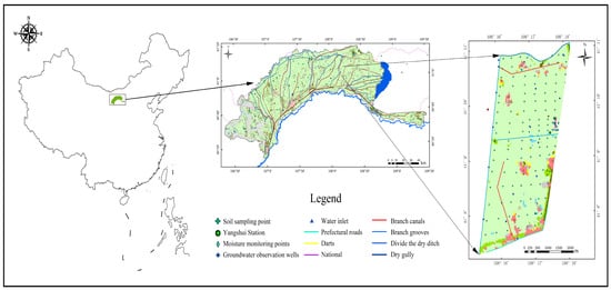
Figure 1.
General geographical features of the study area within the Hetao Irrigation District of China.
Wuyuan County experiences low annual rainfall, which limits natural surface runoff. Consequently, agricultural water demand is predominantly met by the Yellow River, which flows for 59.5 km across the county. The water supply from the Yellow River accounts for approximately 85% of the total water supply, and the water used for irrigation in farmlands constitutes about 80% of the total water consumption. The Yellow River displays pronounced seasonal variability, with discharge ranging from as low as 300–400 m3/s in winter to peaks of 1200–1900 m3/s during the summer flood season. To manage irrigation, two major canals—the Xicheng Canal and the Xiaocheng Canal—are used to distribute water throughout the study area. These canals irrigate approximately 13,750 mu and 6250 mu of farmland, respectively, with annual water withdrawals of 8.1936 million m3 and 3.365 million m3. Groundwater also plays a vital role in the region’s water supply. Groundwater irrigation accounts for approximately 20% to 30% of the total agricultural water usage in the region. Recharge primarily occurs through infiltration from irrigation, precipitation, canal seepage, and lateral seepage from the Yellow River. Groundwater depth typically ranges from 0.5 to 3.2 m, and the aquifer thickness varies between 30 and 160 m, providing a relatively abundant and stable water source for agricultural use.
2.2. Data Collection
2.2.1. Field Observation Data
To ensure representative soil sampling, 90 sampling sites were established across the 20,000 mu experimental area following the principles of randomness, coverage of dominant soil–crop types, logistical accessibility, and long-term monitoring feasibility. Sampling dates were 23 April, 20 May, 29 June, 18 July, 5 August, and 5 September 2021. At each site, soil samples were collected from four depth intervals: 0–20 cm, 20–40 cm, 40–60 cm, and 60–80 cm. GPS coordinates were recorded for all locations. In addition, a fixed monitoring station equipped with a WX-Q2 soil multi-parameter system (Shandong Wanxiang Environmental Technology Co., Ltd., Weifang City, Shandong Province, China) continuously recorded volumetric soil water content. Supplementary sampling campaigns were conducted on 30 June, 23 July, and 21 August 2022 to further capture temporal soil moisture dynamics. Groundwater levels were monitored at 16 sites using HOBO automatic water level loggers (HOBO U20-001-01, Onset Computer Corporation, Cape Cod, MA, USA).
Gravimetric soil moisture content was measured using the oven-drying method (105 °C for 48 h). Air-dried samples were sieved (<0.25 mm) and mixed with distilled water (1:5 ratio) to prepare soil solutions for measuring electrical conductivity (EC), total dissolved solids (TDSs), and salinity. Bulk density was determined using the core method. Particle size distribution was analyzed using a laser particle size analyzer (HELOS-RODOS/M, New Patex Corporation, Hannover City, Lower Saxony, Germany), and soil water retention characteristics were measured using a pressure membrane apparatus and fitted with the van Genuchten model.
2.2.2. Climate Data
Meteorological data served as both input for the HYDRUS-1D model (US Salinity Laboratory, Riverside, CA, USA) and driving data for the data assimilation framework. Daily values of solar radiation, wind speed, precipitation, relative humidity, and maximum and minimum temperatures were collected for April–October 2021 (163 days) and June–August 2022 (63 days) from the Chinese Meteorological Data Sharing Service (http://www.nmic.cn/), accessed on 15 January 2023.
2.2.3. Remote Sensing Data
This study utilized Sentinel-1 and Landsat satellite imagery to support soil moisture inversion and model assimilation. Sentinel-1, part of the European Space Agency’s Copernicus Programme (GMES), comprises two satellites designed for high revisit frequency and extensive spatial coverage. Equipped with C-band Synthetic Aperture Radar (SAR), Sentinel-1 provides all-weather, day-and-night imaging from polar orbits, serving diverse monitoring applications across terrestrial and marine environments. Sentinel-1 data features various polarization modes, including single polarizations (HH: horizontal transmit and horizontal receive; VV: vertical transmit and vertical receive; HV: horizontal transmit and vertical receive; VH: vertical transmit and horizontal receive) and dual-polarization configurations (HH and HV, VV and VH). Additionally, Sentinel-1 operates in four distinct acquisition modes—Stripmap (SM), Interferometric Wide swath (IW), Extra-Wide swath (EW), and Wave mode (WV)—each characterized by unique resolution and swath width capabilities (Table 1). For this study, six Sentinel-1A IW-mode dual-polarization images were selected for optimal surface visibility, acquired on 25 April, 19 May, 1 July, 6 July, 6 August, and 4 September 2021. All radar data were sourced from the ASF DAAC (https://search.asf.alaska.edu), accessed on 15 January 2023.

Table 1.
Root mean square error (RMSE, cm3·cm−3) of simulated soil moisture at four depths (0–20 cm, 20–40 cm, 40–60 cm, 60–80 cm) for each calibration site during the 2021 model calibration period. “Fixed station” refers to the automated soil moisture monitoring site equipped with a WX-Q2 sensor, used for continuous observation and model validation.
The Landsat satellite series, a collaborative program between NASA and the U.S. Geological Survey (USGS), has provided continuous Earth observation data since 1972. With nine satellites launched to date, Landsat data have become essential tools for environmental monitoring, natural resource management, disaster assessment (such as drought), and agricultural applications. This research utilized optical imagery from Landsat 7 (ETM+) and Landsat 8 (OLI/TIRS), captured on 18 April, 20 May, 29 June, 7 July, 16 August, and 17 September 2021. Data were retrieved from the Geospatial Data Cloud (https://www.gscloud.cn) and USGS EarthExplorer (https://earthexplorer.usgs.gov), accessed on 15 January 2023.
Specifically, Sentinel-1A radar data in Level-1 Single Look Complex (SLC) format were utilized, acquired using Interferometric Wide Swath (IW) mode with dual polarization (VV and VH). Radar imagery was preprocessed using the SARscape module within ENVI 5.3 software, involving radiometric calibration to derive accurate backscattering coefficients necessary for soil moisture analysis. Landsat optical remote sensing data were processed in ENVI 5.3 to calculate the normalized difference vegetation index (NDVI), enabling effective vegetation condition estimation for the study area.
Due to inherent remote sensing limitations, soil moisture retrieval was restricted to the surface layer. Consequently, this analysis focused on estimating soil moisture in the 0–20 cm depth range. Following preprocessing, the water cloud model was employed to minimize the effects of vegetation on radar backscatter, thereby improving the accuracy of derived backscattering coefficients. These refined coefficients were subsequently used to construct a soil moisture retrieval model, validated against field-measured soil moisture data.
2.3. Remote Sensing-Based Soil Moisture Retrieval
This study employed radar remote sensing to estimate soil moisture by analyzing backscatter signals captured by the Sentinel-1 Synthetic Aperture Radar (SAR) system. As an active microwave sensor, Sentinel-1 transmits electromagnetic waves toward the Earth’s surface and records the backscattered signals. The strength of this backscatter is influenced by multiple surface properties, most notably soil moisture, surface roughness, and vegetation cover. Because soil dielectric properties are primarily controlled by moisture content, variations in radar backscatter can be used to retrieve soil moisture values.
Radar system parameters such as wavelength, polarization mode, and incidence angle are fundamental in determining the sensitivity of the backscatter to soil conditions. C-band SAR data from Sentinel-1’s Interferometric Wide (IW) mode—offering dual-polarization (VV and VH) and 250 km swath coverage—were selected due to their proven reliability in agricultural applications. To minimize vegetation interference, a water cloud model was used to decouple vegetation effects from soil signals, with the NDVI (derived from Landsat 7/8 imagery) serving as a proxy for vegetation parameters. Generally, the integration of Sentinel-1 radar backscatter and optical vegetation indices allows for more accurate retrieval of surface soil moisture across the moderately saline farmlands of the Hetao irrigation district.
2.4. Water Cloud Model
The water cloud model was proposed by Attema and Ulaby in 1978 [45] and is a widely used semi-empirical model that effectively mitigates the influence of vegetation on soil moisture retrieval from microwave backscatter. By integrating physical mechanisms with statistical relationships, this model improves the accuracy of soil moisture inversion in vegetated areas. The model conceptualizes the vegetative canopy and the underlying soil as two homogeneous, spatially uncorrelated layers. It simplifies the complex processes of microwave absorption and multiple scattering within the canopy by considering only single scattering events. When radar signals interact with the surface, a portion of the microwave energy is directly scattered by the vegetation, while the remaining signal penetrates the canopy, reflects off the soil surface, and then passes back through the vegetation layer before being captured by the radar sensor. During this two-way transmission through the canopy, the radar signal undergoes attenuation due to both scattering and absorption by the vegetation.
The model is mathematically expressed as follows:
where is the two-way transmissivity through the vegetation layer, θ is the radar incidence angle, A and B are empirical parameters determined based on vegetation type, and mV denotes the vegetation water content (kg/m2).
2.5. HYDRUS-1D Model
HYDRUS-1D is a process-based numerical model designed to simulate water, solute, and heat transport in variably saturated porous media [46]. It includes several modules such as water flow, solute transport, root water uptake, and heat transfer. In this study, we primarily utilized the water flow module to simulate one-dimensional vertical soil water dynamics. The model supports a variety of boundary conditions, including constant or variable pressure heads, atmospheric boundaries with ponding and runoff, and specified fluxes [47]. Lower boundary options include free drainage, deep drainage, constant pressure head, and specified flux. Soil hydraulic parameters can be estimated using the Rosetta module, a neural-network-based pedotransfer function that utilizes inputs such as soil texture and bulk density. HYDRUS-1D also includes modules for modeling root water uptake and salinity stress for different plant types.
In this study, the water flow module was used to solve the Richards equation with a source/sink term, simulating water movement through multi-layered, variably saturated soil profiles. Its ability to handle time-varying boundary conditions, flexible input–output interfaces, and integrated parameter optimization functions makes it particularly suitable for modeling unsaturated soil water movement. This module solves the one-dimensional Richards equation augmented by a root-water-uptake sink term, while neglecting air-phase flow and thermal gradients:
where θ represents the volumetric soil water content (cm3·cm−3); t is time (min); z is the vertical spatial coordinate (positive upward); h denotes the pressure head (cm); S is the sink term, representing the volume of water absorbed by plant roots per unit time and per unit volume of soil (cm3·(cm3·d)−1); and K is the unsaturated hydraulic conductivity (cm·d−1). In this study, an atmospheric upper boundary that switches between rainfall, evaporation, infiltration, or ponding and a variable lower boundary for the pressure head driven by the measured groundwater table were chosen. The initial water content profiles were those measured in the field on 26 April 2021.
The hydraulic conductivity is defined by
where Kr is the saturated hydraulic conductivity, and Ks is the relative conductivity. The soil water retention and hydraulic conductivity functions follow the van Genuchten–Mualem model:
The expressions for the parameters in the formula are as follows:
where θs represents the saturated water content (cm3·cm−3), and θr is the residual water content (cm3·cm−3). The values of and are determined from the extrapolated ends of the pressure head–moisture content curve. Generally, ≤ , ≤ . n is the pore distribution index.
The model’s flexible input and output structure allowed us to export simulated pressure heads and water contents in 1 cm increments and to import updated state vectors during ensemble Kalman filter assimilation, making HYDRUS-1D an efficient backbone for the coupled remote sensing data assimilation framework.
By converting the formula, the original Van Genuchten form can be obtained:
(1) Initial and boundary conditions
The initial conditions of the model are the soil moisture content at the start of the simulation period. In this study, the soil moisture contents measured on the initial simulation date of this experiment were adopted.
The HYDRUS-1D model offers three types of boundary conditions for selection, namely, the boundary condition under the condition in which the pressure head is known (the Dirichlet type), the boundary condition under the condition in which the flow rate is known (the Neumann type), and the boundary condition under the condition in which the slope gradient is known.
The known conditions regarding the pressure head are as follows:
The flow rate is known:
The slope gradient is known:
In these formulas, , , and are the pressure head values, and are functions of . is the vector component of the boundary , and points outward.
When selecting the boundary conditions, two main aspects need to be considered: 1. External conditions restrict the soil surface (the soil–atmosphere interface), and the instantaneous moisture condition at the soil surface can determine the actual water flux at this location. 2. The boundary conditions of the soil surface and water flux and the pressure head boundary all change over time; all boundary conditions should be selected based on the actual conditions. To improve the consistency between the numerical solution of the equation and the actual value, the restriction conditions for the soil surface boundary are as follows:
In this formula, represents the water head of the surface pressure in the soil, cm; E represents the potential evaporation rate under the prevailing atmospheric conditions; represents the minimum pressure head under the current soil conditions; and represents the maximum pressure head allowed under the current soil conditions. This value is usually zero. The HYDRUS-1D model assumes that any surface water can be immediately drained.
(2) Characteristic soil hydraulic equation
The van Genuchten model is adopted in the characteristic soil hydraulic equation, and the formula is as follows:
In this formula, is the effective saturation, cm3·cm−3; is the saturated conductivity, cm3·cm−3; is the residual water content, cm3·cm−3; α, m, and n are empirical shape parameters; is the saturated conductivity, cm·d−1; and l is the pore connectivity parameter.
(3) Root water absorption
In this study, the Feddes water stress function is used to describe the root water absorption process. The specific expression is as follows:
In this formula, is the water absorption intensity function, h−1; is the water stress parameter function, dimensionless; is the standardized root water absorption distribution density function, cm−1; and is the crop potential transpiration rate, cm/h.
2.6. Estimation Framework
This study proposes an integrated framework for soil moisture estimation in the Hetao irrigation district, combining remote sensing inversion, process-based modeling, and data assimilation. First, Sentinel-1A and Landsat series satellite images are utilized to derive radar backscatter coefficients by applying the water cloud model (WCM), which minimizes the influence of vegetation on radar signals. Based on the corrected backscatter, an empirical soil moisture retrieval model is constructed and evaluated against field-measured soil moisture data to select the optimal inversion approach for generating spatially distributed soil moisture maps. Second, the HYDRUS-1D model is employed to simulate soil moisture dynamics in agricultural soils. Field-measured soil moisture is used to initialize the model, while daily meteorological inputs—solar radiation, wind speed, precipitation, relative humidity, and maximum and minimum temperatures—serve as boundary conditions. Soil hydraulic parameters are calibrated through laboratory experiments and sensitivity analysis to ensure model accuracy. Third, an ensemble Kalman filter (EnKF) data assimilation scheme is implemented by integrating both remote sensing-derived and in situ soil moisture observations into the HYDRUS-1D model. The assimilation results are compared with non-assimilated simulations to assess improvements in soil moisture estimation accuracy. This framework aims to enhance the reliability of soil moisture monitoring and provide theoretical support for salinization management in irrigated areas of the Hetao Plain. The overall estimation framework is illustrated in Figure 2.
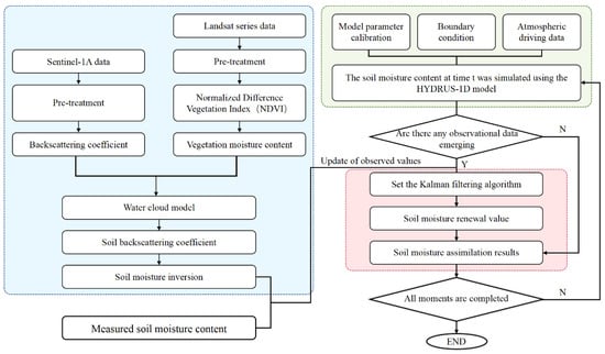
Figure 2.
Framework for soil moisture estimation integrating remote sensing data into the HYDRUS-1D model using the ensemble Kalman filter (EnKF) approach.
3. Results and Discussion
3.1. Performance of the Soil Moisture Retrieval Model
We tested the correlation between surface soil water content and radar backscattering coefficients before and after vegetation correction for both polarizations. In both VV and VH modes, applying the water cloud model markedly improved the correlation, confirming that vegetation effects were effectively suppressed. For VV, the coefficient increased from 0.739 to 0.861 (+0.122); for VH, it rose from 0.649 to 0.770 (+0.121). These results demonstrate that the water cloud model enhances the accuracy of soil moisture retrieval by mitigating crop interference.
In this study, 60 sampling points were used to calibrate four candidate models—linear, quadratic, cubic, and exponential—while the remaining 30 points served for validation (Figure 3). Among the four models, all demonstrated a relatively strong correlation between the VV-polarized backscatter coefficient and soil moisture, with R2 values ranging from 0.7291 to 0.7520. The exponential model performed the worst (R2 = 0.7291), while the cubic model had the highest accuracy (R2 = 0.7520). Thus, the cubic model was selected as the optimal VV-based soil moisture retrieval model. The best-fit equation is y = 0.0006x3 + 0.0184x2 + 0.2061x + 1.0279.
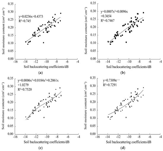
Figure 3.
Comparison of regression models for VV-polarized backscatter versus surface soil moisture content. Soil moisture content (x-axis) is shown in cm3·cm−3; backscattering coefficients (y-axis) are shown in dB. Model equations and fit statistics are displayed in each subplot. (a) Linear model, (b) Quadratic curve model, (c) Trigonometric curve model, and (d) Exponential model.
To assess model accuracy, we used the cubic model for VV polarization to estimate soil moisture at 30 validation sites and compared the results with observed values (Figure 4). Model performance was evaluated using R2, root mean square error (RMSE), and mean relative error (MRE). The VV-based cubic model achieved an RMSE of 0.0213 cm3·cm−3, MRE of 5.54%, and R2 of 0.7964, indicating a high level of accuracy and robustness.
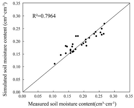
Figure 4.
Validation scatterplot comparing measured and simulated soil moisture content using the VV-polarized cubic regression model. The x-axis shows measured soil moisture (cm3·cm−3), and the y-axis shows simulated values (cm3·cm−3). The coefficient of determination (R2 = 0.7964) indicates strong model agreement.
To evaluate the performance of VH-polarized backscatter data, soil moisture retrieval models were also developed using the same 60 training and 30 validation sample points. Regression models tested included linear, quadratic, cubic, and exponential models. While the cubic model again provided the best fit, the overall performance under VH polarization was notably weaker compared with that under VV polarization, with R2 values ranging from 0.5929 to 0.6342 (Figure S1).
The best-fitting cubic model for VH polarization was y = −0.0004x3 − 0.0237x2 − 0.4264x − 2.1743. Validation yielded an RMSE of 0.0647 cm3·cm−3, MRE of 28.85%, and R2 of 0.59 (Figure S2). These results suggest that VH polarization is less suitable for accurate soil moisture estimation in this region. As such, the VV-polarized cubic model was ultimately selected for this study due to its superior accuracy and reliability.
Using the optimal VV-polarized cubic model, we estimated soil moisture for the study area based on Sentinel-1A imagery collected on 5 August 2021. Soil moisture values were interpolated using kriging in ArcGIS 10.8 (Environmental Systems Research Institute, Inc., Redlands, CA, USA), producing surface soil moisture maps for April through September (Figure 5). Figure 5 reveals that soil moisture was highest in June, July, and August, consistent with the crop growing season and irrigation practices. Rainfall during these months was also higher compared with April and May. A clear spatial trend was observed, with lower moisture in the northern region and higher moisture in the south, highlighting the value of spatial estimates for guiding targeted irrigation.
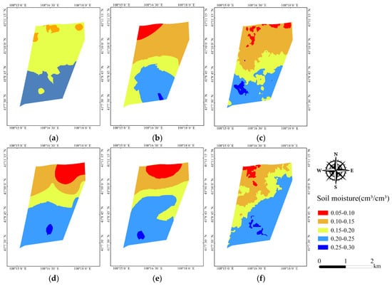
Figure 5.
Estimated surface soil moisture distribution across the study area for the growing season of 2021: (a) April, (b) May, (c) June, (d) July, (e) August, and (f) September. Soil moisture values are expressed in cm3·cm−3. Note: The color scales vary between maps. Areas with higher soil moisture are shown in blue and lower values in red.
3.2. Soil Moisture Simulation Based on the HYDRUS-1D Model
Process-based modeling is essential for soil moisture data assimilation, providing a scientifically robust approach grounded in physically based equations, empirically derived parameters, and experimental validation. In this study, the HYDRUS-1D model was used to simulate soil water dynamics within the Hetao irrigation district. The model utilized meteorological and field-measured soil moisture data, with simulations conducted at a fixed observation station and 16 groundwater monitoring wells. The objective was to capture the vertical distribution and temporal evolution of soil moisture from April to October 2021, providing a reference framework for soil moisture prediction and irrigation management. The vertical soil profile was defined to a depth of 80 cm and divided into four layers (0–20 cm, 20–40 cm, 40–60 cm, and 60–80 cm) based on soil texture and field measurements. Each layer was discretized at 1 cm intervals, creating 81 nodes and 80 computational elements. Monitoring depths were set at 10, 30, 50, and 70 cm. The model simulated a period of 163 days, with an initial time step of 0.001 days and dynamic adjustment ranging from 0.001 to 5 days based on convergence behavior.
The simulation began on 26 April 2021. Initial soil moisture values were based on field measurements taken on that date. Atmospheric boundary conditions were applied at the soil surface, and a variable pressure head boundary was set at the bottom. Daily precipitation, maximum and minimum air temperatures, and other meteorological variables were used as atmospheric drivers.
The HYDRUS-1D model was calibrated using soil moisture data from 2021 and validated using data from 2022. Calibration focused on estimating soil hydraulic parameters using Rosetta’s neural network predictions as initial guesses. The parameters were iteratively adjusted to minimize discrepancies between simulated and observed moisture values. The calibration results (Table 1) showed RMSE values ranging from 0.017 to 0.056 cm3·cm−3, indicating a good match between simulations and observations.
Validation against 2022 data (Table 2) showed similar accuracy, with RMSE values ranging from 0.019 to 0.054 cm3·cm−3, confirming the model’s reliability.

Table 2.
Root mean square error (RMSE, cm3 cm−3) for soil moisture simulation during HYDRUS-1D model validation across 17 sites (2022). RMSE is reported for four depth intervals: 0–20 cm, 20–40 cm, 40–60 cm, and 60–80 cm. Validation includes 16 observation wells (sites #1–#16) and 1 fixed station equipped with continuous sensors.
The calibrated HYDRUS-1D model was applied to simulate soil moisture dynamics at 17 sampling sites (16 wells and 1 fixed station) from April to October 2021. The model produced time-series outputs of soil moisture at four depths (0–20 cm, 20–40 cm, 40–60 cm, and 60–80 cm). The results for sites 1–3 are shown in Figure 6, while the simulation outputs for sites 4–16 and the long-term monitoring site are presented in Figures S3 and S4. Overall, the simulated values were in good agreement with observations, accurately capturing the vertical distribution and temporal variation in soil moisture across the study area.
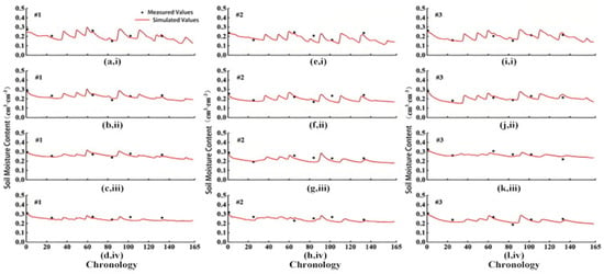
Figure 6.
Comparison of simulated and observed soil moisture content at four depths—(i) 0–20 cm, (ii) 20–40 cm, (iii) 40–60 cm, and (iv) 60–80 cm—for sites 1 to 3 using the calibrated HYDRUS-1D model. Each column of subplots corresponds to one site: (a–d) site 1, (e–h) site 2, and (i–l) site 3. Measured soil moisture is shown as black dots, and simulated values are plotted as red lines. Axes are uniform across subplots for comparability.
As shown in Figure 6 and the Supplementary Materials, Figures S3–S5, the HYDRUS-1D simulations demonstrated a high degree of consistency with measured soil moisture values across different soil depths. Quantitative analysis revealed that the model effectively captured the temporal variations in soil water content throughout the vertical profile, confirming its reliability for hydrological simulations in the study area. Vertical profile analysis revealed a significant increasing trend in soil moisture content with depth, characteristic of the region’s vadose zone dynamics. Surface soil layers (0–20 cm) exhibited pronounced moisture fluctuations, primarily influenced by episodic irrigation events, precipitation patterns (seasonal average 300 mm), and evapotranspiration processes. In contrast, deeper soil horizons (60–100 cm) displayed moisture dynamics predominantly governed by groundwater table fluctuations, showing minimal responsiveness to surface hydrological inputs with variation coefficients below 15%. Temporally, all monitoring points demonstrated marked fluctuation frequency during July-August, corresponding to both peak crop growth stages and intensive irrigation schedules. This period coincided with 63% of annual agricultural water inputs and 45% of precipitation events, creating dynamic soil–plant–atmosphere continuum interactions. The observed moisture variability decreased significantly below 60 cm depth, maintaining relative stability throughout the monitoring period.
Notably, soil moisture varied spatially across sites. According to the simulation results of the model, there are certain differences in the soil moisture levels at the 17 sampling points. For example, well 12 had the highest average surface moisture (0.319 cm3·cm−3). The simulated soil moisture values at well No. 4 demonstrate distinct vertical stratification characteristics, with the surface layer (0–20 cm depth) exhibiting an average moisture content of 0.178 cm3·cm−3, while the deep soil layer (60–80 cm depth) maintains a higher average moisture level of 0.230 cm3·cm−3. This monitoring point exhibits the lowest soil moisture content among all 17 sampling locations, a phenomenon primarily stemming from spatial heterogeneity in environmental parameters including crop species composition, pedological characteristics, and phreatic water table elevation. Furthermore, field investigations revealed significant variations in irrigation schedules and water application rates across different agricultural plots, which constitute additional contributing factors to the observed spatial discrepancies in soil moisture distribution.
The depth-specific simulation results throughout the study period demonstrate that the hydrological model successfully captures the soil moisture dynamics within the research area. These numerical simulations establish a scientific foundation for monitoring agricultural soil moisture variations in the region, while demonstrating satisfactory predictive accuracy that positions the model as a valuable tool for soil water content forecasting in precision agriculture management.
3.3. Soil Moisture Data Assimilation Using the Ensemble Kalman Filter
Although the HYDRUS-1D model demonstrated reliable performance in reproducing long-term soil moisture variation, cumulative errors developed with extended simulation periods. To address this limitation, this section introduces a data assimilation approach that integrates observation data into the simulation framework using the ensemble Kalman filter (EnKF), aiming to improve the accuracy of soil moisture estimation.
Figure 7 shows the assimilation results when incorporating remote sensing and in situ observations. The EnKF assimilation significantly reduced the simulation errors compared with both the raw HYDRUS-1D forecasts and remote sensing estimates. As shown in Figure 8, the RMSE of the assimilated forecasts and analyses using remote sensing were 0.017 and 0.015 cm3·cm−3, respectively, improving upon HYDRUS-1D forecasts by 0.003–0.005 cm3·cm−3. When assimilating in situ observations, the RMSE further dropped to 0.015 and 0.008 cm3·cm−3, indicating higher accuracy. Therefore, in situ assimilation was deemed the optimal strategy and was applied to deeper layers.
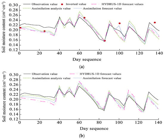
Figure 7.
Surface soil moisture assimilation results using (a) remote sensing and (b) in situ observations. Each panel compares HYDRUS-1D forecasts, assimilation forecasts, and assimilation analyses against observed values (thick black lines). Model outputs are shown using dashed lines of varying thickness.
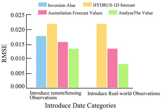
Figure 8.
Root mean square error (RMSE) of surface soil moisture under two assimilation scenarios: (left) remote sensing observations and (right) in situ observations. Bars represent inversion values, HYDRUS-1D forecasts, assimilation forecasts, and assimilation analysis values.
Following the optimized surface assimilation, the EnKF was extended to the 20–40, 40–60, and 60–80 cm layers using the same framework. Assimilation results (Figure 9) showed that model performance improved at all depths. The 20–40 cm layer exhibited moderate fluctuations due to irrigation and rainfall, while deeper layers were relatively stable. Though the assimilation effect diminished with depth, especially below 40 cm, accuracy still improved over the HYDRUS-1D baseline. The results depict the soil moisture assimilation for the 20–80 cm depth layers after incorporating in situ observations into the EnKF algorithm. Figure 9a presents the assimilation results for the 20–40 cm layer. Although soil moisture fluctuations remained evident, indicating sensitivity to external factors such as rainfall and irrigation, the magnitude of variation is less pronounced compared with the surface layer (0–20 cm). The HYDRUS-1D forecast values for this layer generally underestimated soil moisture compared with observations. After assimilation, the analysis values closely align with the observed data, and the assimilation forecasts are slightly more accurate than the HYDRUS-1D predictions, demonstrating an overall improvement in simulation accuracy. Figure 9b,c show the assimilation results for the 40–60 cm and 60–80 cm layers, respectively. Soil moisture at these deeper layers exhibits greater stability with smaller fluctuations, suggesting a reduced response to external influences such as precipitation and irrigation. As seen in the figures, HYDRUS-1D forecasts at these depths also tend to underestimate moisture levels. While data assimilation improves simulation accuracy for both layers, the enhancement is less significant compared with the upper layers (0–20 cm and 20–40 cm).
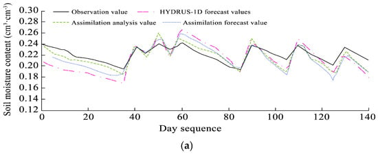
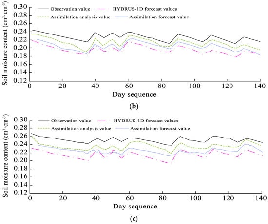
Figure 9.
Soil moisture assimilation results at depth intervals of (a) 20–40 cm, (b) 40–60 cm, and (c) 60–80 cm. Each panel shows HYDRUS-1D forecasts, assimilation forecasts, and assimilation analysis values compared with observed data.
An error analysis was performed on the assimilated soil moisture results (0–80 cm depth) using in situ observations (Table S1). Before assimilation, the HYDRUS-1D model alone showed the largest errors, especially in the 60–80 cm layer, where RE, RMSE, and MAE reached 0.145, 0.037 cm3·cm−3, and 0.037 cm3·cm−3, respectively. After applying the ensemble Kalman filter (EnKF), errors at all depths were significantly reduced, showing a clear improvement in simulation accuracy. Compared with the original HYDRUS-1D forecasts, assimilation forecast values were closer to the observed data. For example, in the 0–20 cm layer, RE, RMSE, and MAE dropped to 0.023, 0.015 cm3·cm−3, and 0.013 cm3·cm−3. The best results were obtained from the assimilation analysis values, which further reduced the errors to 0.016, 0.008 cm3·cm−3, and 0.006 cm3·cm−3. Accuracy generally decreased with depth, but the assimilation still outperformed the original model across all layers. Figure 10 and Figure 11 illustrate the error ranges of soil moisture for four indicators: pre-assimilation error (SP), post-assimilation error (Sa), analysis value (SΔ), and post-assimilation forecast value (SΔa). The difference between HYDRUS-1D forecasts and observations ranged from –0.046 to 0.025 cm3·cm−3 (Figure 10), while assimilation forecasts had smaller differences (–0.036 to 0.019 cm3·cm−3). Figure 11 shows that analysis values were even closer to observations, indicating improved simulation accuracy. Overall, the EnKF-based assimilation method significantly enhanced the reliability of soil moisture estimates and can provide stronger support for farmland water management.
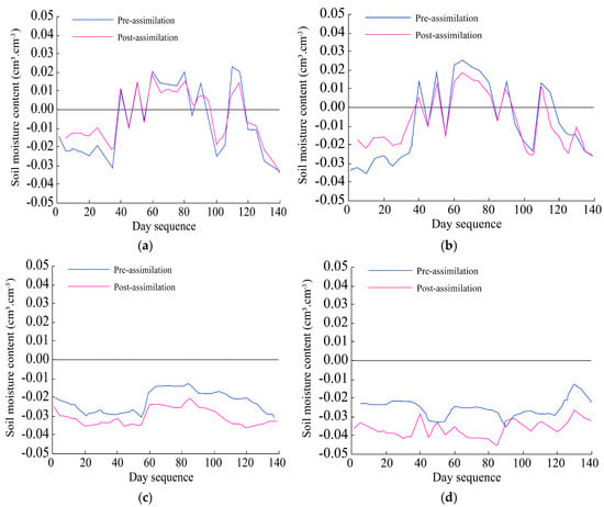
Figure 10.
Differences between model forecasts and observations across dates at four soil depths: (a) 0–20 cm, (b) 20–40 cm, (c) 40–60 cm, and (d) 60–80 cm. Each graph compares pre-assimilation and post-assimilation results across the observation period.
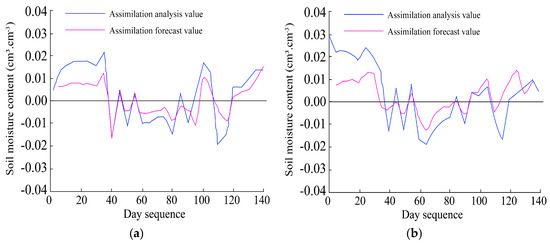
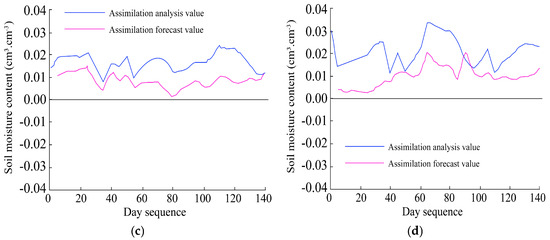
Figure 11.
Differences between soil moisture analysis values and forecast values across dates at four soil depths. Each panel compares assimilation analysis and forecast outputs over the observation period. (a) 0–20 cm, (b) 20–40 cm, (c) 40–60 cm, and (d) 60–80 cm.
4. Discussion
4.1. Comparison with Previous Studies
Soil moisture is a pivotal state variable within terrestrial ecosystems, serving critical functions in both atmospheric regulation and environmental processes. This hydrological parameter exerts a substantial regulatory influence on weather patterns and climatic systems while simultaneously fulfilling essential roles in pedosphere conservation, agricultural productivity, and biogeochemical cycling. Consequently, precise monitoring of soil moisture dynamics bears profound scientific implications and practical value for ecological preservation and the advancement of global sustainability objectives.
Current methodologies for estimating soil moisture encompass three primary approaches: in situ measurements, land surface modeling systems, and remote sensing techniques. Traditional field observations, despite providing direct measurements, exhibit inherent limitations in spatiotemporal coverage due to the parameter’s pronounced spatial heterogeneity and temporal variability. These conventional techniques prove inadequate for comprehensive large-scale monitoring while requiring substantial labor and financial resources. Satellite-based retrieval methods employing radiative transfer models and surface energy balance principles can estimate soil moisture, yet such remote sensing data only capture transient surface conditions during satellite overpasses, resulting in temporal discontinuities and inherent physical inconsistencies, particularly regarding water and energy balance discrepancies.
Land surface process models and hydrological simulation frameworks offer a continuous temporal representation of soil moisture dynamics through numerically solving coupled water and energy equations. However, model structural deficiencies, parameterization uncertainties, and inaccuracies in forcing variables frequently lead to substantial simulation errors. This methodological trilemma underscores the critical need for innovative approaches that synergize observational data with physical models while maintaining thermodynamic consistency. The current scientific challenge, therefore, necessitates the development of an optimized methodology for soil moisture estimation capable of reconciling observational accuracy with physically consistent temporal continuity.
An et al. [48] developed a machine learning (ML) framework that fills the temporal gaps in the soil moisture (SM) gathered by the Soil Moisture Active and Passive (SMAP) mission during 1–3-day satellite revisit intervals by generating real-time SM estimates at 36 km resolution in the Hengduan Mountain region (HDMR). The long short-term memory (LSTM) network model was identified as the top performer. It was also found that sparse vegetation regions show a higher accuracy of inversion compared to dense vegetation regions. Shahriari et al. [49] proposed a seasonal approach to estimating surface soil moisture at 10 m resolution using a combination of Synthetic Aperture Radar (SAR) and optical imagery coupled with two machine learning algorithms: Support Vector Regression (SVR) and Random Forest (RF). This approach offers promising enhancements in soil moisture monitoring, with a 0.002 m3/m3 reduction in RMSE and a 0.03 increase in correlation, potentially advancing our understanding and management of this critical environmental variable across various applications. However, the potential uncertainty introduced by the time lag between Sentinel-1 and Sentinel-2 acquisitions due to dynamic changes in vegetation water content should be acknowledged as a limitation. Qian et al. [50] used dual-polarization C-band radar data as the core to construct a multi-layer and SM profile estimation framework. Validation was carried out in two new SM observation networks: the Qinghai Lake basin (QLB-NET) and the Heihe River basin (WATERNET). The results showed that the multi-output and -input stacking strategy regression (SSR) model demonstrated excellent spatiotemporal extensibility and interannual transferability in multi-layer and profile SM estimation. However, this framework is constrained by the multi-source auxiliary data (optical vegetation descriptors, soil properties, and terrain factors). The above-mentioned methods continue to be restricted by elements such as plant cover, terrain unevenness, and low depth resolution. These problems prove especially acute in saltwater-irrigated areas, where intense evaporation and pronounced surface reflectivity amplify measurement inaccuracies. These deficiencies can be addressed by using data assimilation techniques to integrate multi-sensor Earth observation data with computational simulations.
Data assimilation technology was originally developed and extensively applied in atmospheric and oceanic sciences. In recent decades, this methodology has been progressively extended to hydrological research domains, particularly in soil moisture modeling. The fundamental strength of this approach resides in its capacity to systematically integrate multi-source observational data characterized by heterogeneous temporal–spatial resolutions and measurement accuracies, while simultaneously incorporating numerical model simulations. More significantly, the framework enables quantitative assessment of error uncertainties through rigorous comparison with model forecast uncertainties in state variables, thereby facilitating continuous calibration of soil moisture predictions and progressive enhancement of model simulation accuracy. Contemporary research demonstrates that numerous scholars have successfully implemented various data assimilation algorithms in hydrological modeling applications. Notable implementations include Kalman filter (KF), Simulated Annealing algorithms, and ensemble Kalman filter (EnKF) methodologies. These hybrid modeling frameworks that couple advanced assimilation techniques with hydrological models have shown substantial improvements in soil moisture simulation accuracy, as evidenced by multiple validation studies across different spatial scales and climatic conditions.
Vahidi et al. [51] conducted depth-specific soil moisture estimation in vegetated corn fields using a canopy-informed model via fusion of RGB–thermal drone data and machine learning. Their results reveal that thermal variables, particularly LST, exhibit significant correlations with soil moisture at shallower depths, especially in non-irrigated plots where moisture variability tends to be greater. The GBM model performed exceptionally well, achieving a coefficient of determination (R2) of 0.79 and a root mean square error (RMSE) of 1.86 % at a depth of 10 cm, showcasing its precision in moisture prediction. However, LST’s effectiveness in predicting soil moisture decreased, underscoring the dynamic interaction between plant growth stages and moisture estimation accuracy. Panzeri et al. [52] proposed a method coupling a modified ensemble Kalman filter (EnKF) algorithm with stochastic moment equations (MEs) governing space–time variations in (theoretical ensemble) mean and covariance values of groundwater flow state variables (hydraulic heads and fluxes). Whereas traditional EnKF entails Monte Carlo (MC) simulations and suffers from inbreeding, their approach avoids both issues. Chenting Jiang et al. [53] proposed the EnKF-fsolve model, which merges the fsolve function with the ensemble Kalman filter (EnKF) to simultaneously simulate sequenced soil moisture and predict hydraulic parameters of the van Genuchten–Mualem (VGM) model at multiple soil depths. This model demonstrated superior convergence, computational efficiency, and simulation accuracy. The outstanding performance of the EnKF-fsolve model was attributed to the dynamic optimization procedure and parallel computational operations of the EnKF, as well as its consideration of model and observational uncertainties in highly nonlinear soil water systems. When compared to previous research findings, the ensemble Kalman filter (EnKF) algorithm demonstrates significant advantages when integrated with hydrological models for data assimilation applications. This combined approach not only provides optimal estimation but also quantifies specific confidence intervals, rendering it particularly suitable for soil moisture estimation studies. However, current research exhibits a critical knowledge gap regarding parameterized data assimilation schemes that combine the EnKF algorithm with diverse hydrological models. Specifically, no comprehensive investigation has been conducted on this methodological integration for soil moisture estimation in saline–alkali farmland ecosystems within China’s Hetao Irrigation Area.
This investigation showed that the simulation precision of the HYDRUS-1D model was significantly enhanced for layered soil moisture through the integration of observational data with the ensemble Kalman filtering algorithm. This study further examined the impacts of ensemble dimensionality and the observational error magnitude on the accuracy of soil moisture estimations. The results demonstrated that moderately increasing the ensemble size effectively diminishes the root mean square error (RMSE) of soil water simulations, whereas excessively large ensembles led to negligible improvements in accuracy while compromising the computational efficiency. Additionally, the observational error exerted a substantial influence on the accuracy of soil moisture estimations, with reduced error values correlating directly to a lower simulation RMSE. Current research predominantly validates data assimilation techniques by comparing model simulations, assimilated analyses, and measured values. This study uniquely investigates whether temporal assimilation processes enhance the forecasting accuracy. After incorporating assimilation-predicted values into comparative analyses, the findings reveal that these forecasts exhibit closer alignment with observed values than standalone HYDRUS-1D predictions, thereby confirming that current-time assimilation is able to optimize model forecasts.
4.2. Limitations and Future Framework
Although our study achieved meaningful progress in soil moisture retrieval and simulation, several limitations remain. First, due to the lack of field measurements for surface vegetation parameters, the water cloud model relied on empirical A and B coefficients from previous studies, which may have reduced inversion accuracy. Future work should involve field-based measurements of plant height, leaf area index, and vegetation water content to refine these parameters and improve model performance. Second, the HYDRUS-1D model used fixed soil hydraulic parameters throughout the simulation, which may not reflect real-time changes in soil properties. Incorporating time-varying or adaptive parameterizations in future research could enhance the accuracy of soil moisture simulations. Third, the current retrieval relied on medium-resolution remote sensing data (e.g., Sentinel-1A, Landsat). The integration of higher-resolution optical and active microwave data (e.g., GF-2, QuickBird, GF-3, ALOS-2) is recommended to improve spatial accuracy and potentially reduce dependence on in situ observations in data assimilation. Lastly, the current data assimilation was limited to point-scale applications; future studies should enhance sampling density and extend assimilation to spatial scales to support broader soil moisture monitoring and farmland management in the Hetao irrigation district.
5. Conclusions
This study proposed a multi-source soil moisture estimation framework that integrates Sentinel-1 remote sensing data, the HYDRUS-1D vadose zone model, and ensemble Kalman filtering (EnKF) data assimilation.
- (1)
- Vegetation effects were corrected using the water cloud model, and a cubic regression model based on VV polarization achieved the best performance for soil moisture retrieval (R2 = 0.7964, RMSE = 0.0213 cm3·cm−3).
- (2)
- The HYDRUS-1D model was calibrated and validated using multi-depth field observations. The results confirmed the model’s ability to capture vertical soil moisture dynamics with RMSEs ranging from 0.017 to 0.056 cm3·cm−3 across soil layers, indicating good agreement with observed values.
- (3)
- Third, EnKF-based data assimilation was applied using both remote sensing and in situ soil moisture data. Assimilation significantly improved simulation accuracy, particularly at a depth of 0–20 cm. Among the two data sources, assimilation with in situ measurements yielded higher accuracy and was thus used for deeper soil layers. The assimilation analysis values consistently outperformed both the raw model predictions and forecast ensemble means, highlighting the strength of the EnKF approach.
Generally, this study enhances the accuracy of soil moisture estimation in irrigated agricultural regions, offering valuable guidance for precision water management and long-term soil monitoring in the Hetao irrigation district.
Supplementary Materials
The following supporting information can be downloaded at https://www.mdpi.com/article/10.3390/agriculture15121320/s1 Figure S1: Validation scatterplot comparing measured and simulated soil moisture (VV polarization); Figure S2: Validation scatterplot comparing measured and simulated soil moisture (VH polarization); Figure S3: Same as Figure 6 but for sites 4–9; Figure S4: Same as Figure 6 but for sites 10–15; Figure S5: Same as Figure 6 but for sites 16 and fixed station; Table S1: Error statistics (RE, RMSE, MAE) for HYDRUS-1D forecast, assimilation forecast, and analysis values at different soil depths.
Author Contributions
All authors contributed to the conception and design of the study. Y.S.: Conceptualization, data analysis, and manuscript drafting and revision. Q.L. (Quanming Liu): Conceptualization and manuscript review and critical revision for important intellectual content. C.W.: Conceptualization, experimental design, sample collection, and chemical analysis. Q.L. (Qi Liu): Conceptualization, experimental design, sample collection, and chemical analysis. Z.Q.: Manuscript review and critical revision for important intellectual content. All authors have read and agreed to the published version of the manuscript.
Funding
This research was jointly supported by the National Key Research and Development Program of China (No. 2021YFC3201205 and No. 2021YFD1900605), the project for Construction of Leading Talents and Innovative Teams in Science and Technology in Inner Mongolia Autonomous Region (BR22-13-12) and Natural Science Foundation Project of Inner Mongolia Autonomous Region (2025MS05114).
Institutional Review Board Statement
This study did not involve humans or animals.
Data Availability Statement
Publicly available datasets (Sentinel-1, Landsat, meteorological data) were used in this study and can be accessed at https://search.asf.alaska.edu, https://earthexplorer.usgs.gov, and https://sci.cma.cn/, accessed on 15 January 2023. Field observation data are available from the corresponding author upon reasonable request.
Acknowledgments
We would like to thank the editors and the anonymous reviewers for their work, helpful suggestions, and comments.
Conflicts of Interest
The authors declare that they have no conflicts of interest.
References
- Yin, M.; Jiang, Y.; Ling, Y.; Ma, Y.; Qi, G.; Kang, Y.; Wang, Y.; Lu, Q.; Shang, Y.; Fan, X.; et al. Optimizing lucerne productivity and resource efficiency in China’s yellow river irrigated region: Synergistic effects of ridge-film mulching and controlled-release nitrogen fertilization. Agriculture 2025, 15, 845. [Google Scholar] [CrossRef]
- Rodell, M.; Famiglietti, J.S. Detectability of variations in continental water storage from satellite observations of the time dependent gravity field. Water Resour. Res. 1999, 35, 2705–2723. [Google Scholar] [CrossRef]
- Seneviratne, S.I.; Corti, T.; Davin, E.L.; Hirschi, M.; Jaeger, E.B.; Lehner, I.; Orlowsky, B.; Teuling, A.J. Investigating soil moisture–climate interactions in a changing climate: A review. Earth Sci. Rev. 2010, 99, 125–161. [Google Scholar] [CrossRef]
- Yao, Y.; Yan, J.; Li, G.; Ma, W.; Yao, X.; Song, M.; Li, Q.; Li, J. A GNSS-IRsoil moisture inversion method considering multi-factor influences under different vegetation covers. Agriculture 2025, 15, 837. [Google Scholar] [CrossRef]
- Farrell, M.; Leizica, E.; Gili, A.; Noellemeyer, E. Identification of management zones with different potential moisture availability for sustainable intensification of dryland agriculture. Precis. Agric. 2023, 24, 1116–1131. [Google Scholar] [CrossRef]
- Ju, W.; Gao, P.; Wang, J.; Zhou, Y.; Zhang, X. Combining an ecological model with remote sensing and GIS techniques to monitor soil water content of croplands with a monsoon climate. Agric. Water Manag. 2010, 97, 1221–1231. [Google Scholar] [CrossRef]
- Feddes, R.A.; Menenti, M.; Kabat, P.; Bastiaanssen, W.G.M. Is large-scale inverse modelling of unsaturated flow with areal average evaporation and surface soil moisture as estimated from remote sensing feasible? J. Hydrol. 1993, 143, 125–152. [Google Scholar] [CrossRef]
- Yu, F.; Li, H.T.; Zhang, C.M.; Wen, X.F.; Gu, H.Y.; Han, Y.S.; Lu, X.J. Data assimilation on soil moisture content based on multi-source remote sensing and hydrologic model. J. Infrared Millim. Waves 2014, 33, 602–607. [Google Scholar]
- Liu, Z.; Zhou, Y.L.; Ju, W.M.; Gao, P. Simulation of cropland soil moisture based on an ensemble Kalman filter. Chin. J. Appl. Ecol. 2011, 22, 2943–2953. [Google Scholar] [CrossRef]
- Zhang, G. Data Assimilation of Soil Moisture in Farmland in Low Hill Red Soil Region Based On SiB2 and Kalman Filter. Master’s Thesis, Nanjing University of Information Science and Technology, Nanjing, China, 2018. [Google Scholar]
- Muzylev, E.L. Utilization of remote sensing data in the simulation of the water and heat regime of land areas: A review of publications. Water Resour. Res. 2023, 50, 709–731. [Google Scholar] [CrossRef]
- Petropoulos, G.P.; Ireland, G.; Barrett, B. Surface soil moisture retrievals from remote sensing: Current status, products & future trends. Phys. Chem. Earth 2015, 83–84, 36–56. [Google Scholar] [CrossRef]
- Cheng, T.; Hong, S.; Huang, B.; Qiu, J.; Zhao, B.; Tan, C. Passive microwave remote sensing soil moisture data in agricultural drought monitoring: Application in northeastern China. Water 2021, 13, 2777. [Google Scholar] [CrossRef]
- Xu, P.; Zhang, C. Research progress on remote sensing inversion of soil moisture. For. Resour. Manag. 2015, 151–156, 160. [Google Scholar] [CrossRef]
- Bowers, S.A.; Hanks, R.J. Reflection of radiant energy from soil. Soil Sci. 1971, 100, 130–138. [Google Scholar] [CrossRef]
- Guo, G.; Zhao, B. Monitoring soil moisture using MODIS data. Soil 2004, 219–221. [Google Scholar] [CrossRef]
- Verstraeten, W.W.; Veroustraete, F.; van der Sande, C.J.; Grootaers, I.; Feyen, J. Soil moisture retrieval using thermal inertia, determined with visible and thermal spaceborne data, validated for European forests. Remote Sens. Environ. 2006, 101, 299–314. [Google Scholar] [CrossRef]
- Price, J.C. On the analysis of thermal infrared imagery: The limited utility of apparent thermal inertia. Remote Sens. Environ. 1985, 18, 59–73. [Google Scholar] [CrossRef]
- Zhang, R. Thermal capacity model of soil moisture content and its application. Chin. Sci. Bull. 1991, 36, 924–927. [Google Scholar] [CrossRef][Green Version]
- Baioni, E.; Fiantanese, G.; Porta, G.M. Data-driven assessment of climate change and vegetative cover dynamics in traditional oases. J. Hydrol. Reg. Stud. 2025, 59, 102266. [Google Scholar] [CrossRef]
- Cai, Q.; Li, E.; Tao, L.; Jiang, R. Farmland soil moisture retrieval using PROSAIL and water cloud model. Trans. Chin. Soc. Agric. Eng. 2018, 34, 117–123. [Google Scholar] [CrossRef]
- Belmans, C.; Wesseling, J.G.; Feddes, R.A. Simulation model of the water balance of a cropped soil: SWATRE. J. Hydrol. 1983, 63, 271–286. [Google Scholar] [CrossRef]
- Chen, F.; Dudhia, J. Coupling an advanced land surface–hydrology model with the Penn State–NCAR MM5 modeling system. Part I: Model implementation and sensitivity. Mon. Weather Rev. 2001, 129, 569–585. [Google Scholar] [CrossRef]
- Guo, Q.L.; Li, J.L. Dynamic simulation of soil moisture in rain-fed winter wheat farmland based on BEPS model. J. Irrig. Drain. 2017, 36, 1–7. [Google Scholar] [CrossRef]
- JIANG, B.; TIAN, J.; SU, H. Estimation of monthly evapotranspiration and soil moisture in the Central Asia. Prog. Geogr. 2020, 39, 433–442. [Google Scholar] [CrossRef]
- Ju, W.; Chen, J.M.; Black, T.A.; Barr, A.G.; Liu, J.; Chen, B. Modelling multi-year coupled carbon and water fluxes in a boreal aspen forest. Agric. For. Meteorol. 2006, 140, 136–151. [Google Scholar] [CrossRef]
- Liu, J. A process-based boreal ecosystem productivity simulator using remote sensing inputs. Remote Sens. Environ. 1997, 62, 158–175. [Google Scholar] [CrossRef]
- Zhao, Z.B.; Jin, R.; Tian, W.; Kang, J.; Su, Y. Applicability research of indices in soil moisture downscaling based on SiB2 simulation. Remote Sens. Tech. Appl. 2017, 32, 195–205. [Google Scholar] [CrossRef]
- Li, B.B.; Wang, Y.Q.; Li, Z. Applicability of HYDRUS-1D model in simulating the soil moisture in deep profiles on the Weibei rainfed highland, China. Chin. J. Appl. Ecol. 2019, 30, 398–404. [Google Scholar] [CrossRef]
- Li, Q.; Li, F.; Zhang, Q.; Qiao, Y.; Du, K.; Zhu, N.; Yang, G.; Li, J.; He, X. Water and salt transport simulation in the wheat growing area of the North China Plain based on HYDRUS model. Chin. J. Eco-Agric. 2021, 29, 1085–1094. [Google Scholar] [CrossRef]
- Bosilovich, M.G.; Radakovich, J.D.; da Silva, A.; Todling, R.; Verter, F. Skin temperature analysis and bias correction in a coupled land-atmosphere data assimilation system. Water Resour. Res. 2007, 85, 205–228. [Google Scholar] [CrossRef]
- Huang, J.; Song, J.; Huang, H.; Zhuo, W.; Niu, Q.; Wu, S.; Ma, H.; Liang, S. Progress and perspectives in data assimilation algorithms for remote sensing and crop growth model. Sci. Remote Sens. 2024, 10, 100146. [Google Scholar] [CrossRef]
- Ma, J.; Qin, S. Recent advances and development of data assimilation algorithms. Adv. Earth Sci. 2012, 27, 747–757. [Google Scholar]
- Margulis, S.A.; McLaughlin, D.; Entekhabi, D.; Dunne, S. Land data assimilation and estimation of soil moisture using measurements from the Southern Great Plains 1997 Field Experiment. Water Resour. Res. 2002, 38, 35-1–35-18. [Google Scholar] [CrossRef]
- McLaughlin, D. An integrated approach to hydrologic data assimilation: Interpolation, smoothing, and filtering. Adv. Water Resour. 2002, 25, 1275–1286. [Google Scholar] [CrossRef]
- Pipunic, R.; Walker, J.; Western, A. Assimilation of remotely sensed data for improved latent and sensible heat flux prediction: A comparative synthetic study. Remote Sens. Environ. 2008, 112, 1295–1305. [Google Scholar] [CrossRef]
- Evensen, G. Data Assimilation: The Ensemble Kalman Filter; Springer: Berlin/Heidelberg, Germany, 2009. [Google Scholar]
- Li, X.; Toshio, K.; Cheng, G. An algorithm for land data assimilation by using simulated annealing method. Adv. Earth Sci. 2003, 18, 632–636. [Google Scholar]
- Nagarajan, K.; Judge, J.; Graham, W.D.; Monsivais-Huertero, A. Particle Filter-based assimilation algorithms for improved estimation of root-zone soil moisture under dynamic vegetation conditions. Adv. Water Resour. 2011, 34, 433–447. [Google Scholar] [CrossRef]
- Walker, J.P.; Willgoose, G.R.; Kalma, J.D. One-dimensional soil moisture profile retrieval by assimilation of near-surface observations: A comparison of retrieval algorithms. Adv. Water Resour. 2001, 24, 631–650. [Google Scholar] [CrossRef]
- Ding, J.; Chen, W.; Wang, L. Improving monitoring precision of soil moisture by assimilation of HYDRUS model and remote sensing-based data by ensemble Kalman filter. Trans. Chin. Soc. Agric. Eng. 2017, 33, 166–172. [Google Scholar] [CrossRef]
- HUANG, C.; LI, X. Sensitivity analysis on land data assimilation scheme of soil moisture. Adv. Water Sci. 2006, 17, 457–465. [Google Scholar] [CrossRef]
- Wang, W.; Liu, Y.W.; Kou, X.H.; Lu, H.S. EnKF and HYDRUS-1 D based data assimilation experiments for improving soil moisture profile prediction. J. Hydraul. Eng. 2012, 43, 1302–1311. [Google Scholar] [CrossRef]
- Gupta, S.K.; Singh, S.K.; Kanga, S.; Kumar, P.; Meraj, G.; Sahariah, D.; Debnath, J.; Chand, K.; Sajan, B.; Singh, S. Unearthing India’s soil moisture anomalies: Impact on agriculture and water resource strategies. Theor. Appl. Climatol. 2024, 155, 7575–7590. [Google Scholar] [CrossRef]
- Attema, E.P.W.; Ulaby, F.T. Vegetation modeled as a water cloud. Radio Sci. 1978, 13, 357–364. [Google Scholar] [CrossRef]
- Juhászné, A.C.; Sarkadi, N.; Czigány, S.; Geresdi, I. Contribution of surface evaporation to winter fog formation: Numerical simulation of water transport in silty soils of SW Hungary using the Hydrus-1D model. J. Hydrol. Reg. Stud. 2025, 59, 102397. [Google Scholar] [CrossRef]
- Li, Y.; Yu, Q.; Ning, H.; Gao, Y.; Sun, J. Simulation of soil water, heat, and salt adsorptive transport under film mulched drip irrigation in an arid saline-alkali area using HYDRUS-2D. Agric. Water Manag. 2023, 290, 108585. [Google Scholar] [CrossRef]
- An, H.; Ouyang, C.; Chen, X. Real-time estimation of SMAP soil moisture in mountainous areas and its impact on rainfall-runoff simulation. J. Hydrol. 2025, 660, 133487. [Google Scholar] [CrossRef]
- Shahriari, M.A.; Aghighi, H.; Azadbakht, M.; Ashourloo, D.; Matkan, A.A.; Brakhasi, F.; Walker, J.P. Soil moisture estimation using combined SAR and optical imagery: Application of seasonal machine learning algorithms. Adv. Space Res. 2025, 75, 6207–6221. [Google Scholar] [CrossRef]
- Qian, J.; Yang, J.; Sun, W.; Zhao, L.; Shi, L.; Shi, H.; Liao, L.; Dang, C.; Dou, Q. Evaluation and improvement of spatiotemporal estimation and transferability of multi-layer and profile soil moisture in the Qinghai Lake and Heihe River basins using multi-strategy constraints. Geoderma 2025, 455, 117222. [Google Scholar] [CrossRef]
- Vahidi, M.; Shafian, S.; Frame, W.H. Depth-specific soil moisture estimation in vegetated corn fields using a canopy-informed model: A fusion of RGB-thermal drone data and machine learning. Agric. Water Manag. 2025, 307, 109213. [Google Scholar] [CrossRef]
- Panzeri, M.; Riva, M.; Guadagnini, A.; Neuman, S.P. EnKF coupled with groundwater flow moment equations applied to Lauswiesen aquifer, Germany. J. Hydrol. 2015, 521, 205–216. [Google Scholar] [CrossRef]
- Jiang, C.; Hardie, M.; West, D.; Bai, Q.; Page, D. A hybrid EnKF-fsolve model for simultaneous dynamic soil moisture simulation and hydraulic parameters prediction. J. Hydrol. 2025, 660, 133242. [Google Scholar] [CrossRef]
Disclaimer/Publisher’s Note: The statements, opinions and data contained in all publications are solely those of the individual author(s) and contributor(s) and not of MDPI and/or the editor(s). MDPI and/or the editor(s) disclaim responsibility for any injury to people or property resulting from any ideas, methods, instructions or products referred to in the content. |
© 2025 by the authors. Licensee MDPI, Basel, Switzerland. This article is an open access article distributed under the terms and conditions of the Creative Commons Attribution (CC BY) license (https://creativecommons.org/licenses/by/4.0/).