Study of Volatility Spillover from Crude Oil Futures to Grain Futures Across Multiple Cycles Based on the EEMD-BEKK-GARCH Model

Abstract

Against the backdrop of increasing financialization of grain markets, the cross-cycle and cross-market contagion among commodities has been intensifying. To investigate the risk spillover among commodities across different cycles, this study selected UK WTI crude oil and soybean, corn, and wheat futures prices from the Chicago Board of Trade as research subjects. Using ensemble empirical mode decomposition (EEMD), the original sequences were decomposed into sub-sequences of different frequencies. Based on these frequency characteristics, long-term, medium-term, and short-term fluctuations were constructed. The BEKK-GARCH model was then applied to explore the volatility spillover across markets under different cycles. The results indicate that in terms of pricing mechanisms, crude oil futures dominate the price fluctuations of grain futures. In terms of risk spillover across different cycles, there is a bidirectional risk spillover effect between crude oil and grain futures in short-term and medium-term fluctuations, while in long-term fluctuations, there is only a unidirectional transmission from crude oil futures to grain futures. Based on the research findings, this paper proposes relevant policy recommendations, aiming to provide government regulatory authorities and futures investors with policy guidance and a theoretical foundation across different cycles.

1. Introduction

With the development of the global economy, the international futures market has expanded rapidly. According to the Futures Industry Association (FIA), the global trading volume of futures and options reached a record 137.5 billion contracts in 2023, an increase of 53.445 billion contracts compared to 2022, reflecting a year-on-year growth of 64%. The commodity market showed a general upward trend, with double-digit increases in transaction volumes across the board. Energy and agricultural commodity futures saw transaction growth of over 30% (data from https://www.cfachina.org/industrydynamics/mediaviewoffuturesmarket/202402/t20240207_67416.html (accessed on 19 December 2024)). However, the increasing risk interconnection between financial markets will lead to large capital inflows or outflows, reducing the stability of the financial system. When hit by negative information, the expectations of returns and risk aversion among financial market participants will amplify financial risks [1,2], leading to increased cross-market risk contagion across various financial markets [3,4]. Commodity price fluctuations are no longer solely determined by supply and demand; price risks caused by cross-cycle and cross-market shocks are becoming increasingly severe [5,6,7,8]. As crucial investment and risk-hedging instruments, crude oil and grain futures price volatility will significantly impact investment trends and international import risks [9,10]. Moreover, as crucial strategic commodities, large price fluctuations in crude oil and grain can lead to global hunger and economic and social instability [11,12]. Therefore, understanding and managing the risk transmission mechanisms between crude oil futures and biofuel-producing grain futures can help stabilize market sentiment, reduce international investor sentiment fluctuations, and in turn mitigate the negative impact on the real economy. Thus, it is crucial to deeply understand the price determination mechanisms and asymmetric transmission effects between global crude oil and grain futures across different cycles.

The price impact of crude oil futures on grain futures has attracted significant scholarly attention. The first approach predominantly includes cointegration, error correction models, and VAR models, which primarily aim to test the causality of market price changes [13,14]. The second approach is the information spillover effect model, which examines the impact of the direction of information flow within each market and posits that markets with stronger information spillover have a guiding influence on prices [15]. Given the challenges of accurately measuring pricing effectiveness or determining the market’s share of contribution to the pricing system, some scholars have proposed information share (IS) and permanent transitory (PT). The permanent transitory (PT) model is a time-series analysis method aimed at distinguishing between the permanent component and the transitory component of a market variable. The permanent component represents long-term, structural changes. In contrast, the transitory component is driven by short-term shocks, such as seasonal factors or unexpected events, which typically revert over time. These models are used to assess the influence of each market on prices, thereby determining each market’s pricing power [16]. In the context of multi-scale decomposition, Fourier transform (FT), wavelet transform (WT), and the mixed data sampling regression model (MIDAS) are commonly employed in the analysis of risk transmission in financial markets [17,18,19,20]. These methods are used to analyze the characteristics of high-frequency and low-frequency transmission between markets by capturing different frequency components. However, wavelet decomposition is sensitive to the selection of model parameters, making the decomposition results more subjective, and there has been limited investigation into the volatility spillover effects across different scales.

Existing literature on the pricing power of futures prices reveals three main areas for further improvement. First, most studies focus on a single time scale, lacking multi-scale analysis. However, crude oil and grain futures are commodities with inherent heterogeneity, and their price fluctuations are influenced by macroeconomic factors, geopolitics, supply and demand, financial speculation, and other variables at different scales [21,22,23]. Consequently, their risk evolution may exhibit multi-scale characteristics, making it essential to analyze price evolution from a multi-dimensional perspective. Secondly, multi-scale decomposition algorithms often exhibit greater subjectivity, and the decomposition sequences may fail to capture key features of the original time series, leading to incomplete analysis. Furthermore, some algorithms may result in a lower degree of reduction, causing the analysis to deviate from the original sequence. Third, there is insufficient research on serial volatility spillovers after multi-scale decomposition, which fails to systematically elucidate the multi-scale volatility spillovers of price-influencing factors. There are differences in the information transmission effect of commodities at different time scales and heterogeneity in the information transmission ability at each scale. However, the impact of the pricing power of crude oil futures on grain futures has not been studied on different time scales, thus making it difficult to provide policymakers with precise guidance for making short-, medium-, and long-term investment decisions or regulatory policies.

The main contributions of this paper are as follows. First, the information share model is employed to analyze the long-term dominant relationship and information share size of crude oil and three grain futures under long-term cointegration, thereby expanding the application scenarios of the information share model and enhancing the robustness of the pricing results. Second, the EEMD method is applied to decompose and reconstruct each time series into high-frequency, low-frequency, and trend terms, which addresses the deficiencies in time series decomposition in existing studies, accurately captures the characteristics of time series at different scales, and helps construct a volatility characterization system across different cycles. Third, the BEKK-GARCH model [24,25,26] is employed to empirically analyze the size and direction of the risk spillover effect between crude oil futures and grain futures across different frequency domains, thereby enriching the study of volatility spillover in different scales of energy and agricultural product futures markets and providing methodological insights for analyzing volatility spillover effects across cycles using frequency domain techniques.

The structure of the paper is as follows: Section 2 provides an overview of the research methodology, Section 3 introduces the methodological principles, Section 4 describes the raw data and the process of decomposition and reorganization, Section 5 presents the empirical results, and Section 6 concludes with the conclusions and recommendations.

2. Multi-Scale Characterization of Crude Oil and Grain Futures

At a time when the financialization of global commodities is increasing, the causes of food crises are primarily not due to imbalances in supply and demand fundamentals but rather the result of a combination of non-traditional factors, including the financialization of food, food energy integration, and international speculation. The food market is highly interconnected with both the financial and energy markets, particularly in the context of the rapid development of food futures and other derivative markets. As a result, international food prices have become increasingly sensitive to changes in financial variables such as money supply, interest rates, and other commodities. At the same time, the crude oil futures market is the largest commodity futures derivative market in the world, and crude oil futures are classified as highly financialized, allowing them to more accurately capture fluctuations in international risks. As crude oil is a key anchor for the US dollar, it also better responds to fluctuations in global monetary policy. Moreover, chemical products derived from crude oil as basic raw materials are used across all aspects of agricultural production, meaning fluctuations in crude oil futures are linked to fluctuations in grain futures prices. This creates a linkage effect between fluctuations in crude oil futures and grain futures prices.

In the study of the impact of crude oil and international grain futures, the financial market’s impact exhibits various characteristics, including industry asymmetry, transience, and persistence [27,28]. Existing research indicates that the dynamic impact of different events on the financial market differs significantly, with crude oil futures affecting grain futures price changes through three main channels. First, from a macro-level perspective, the degree of macroeconomic development influences the demand for crude oil, which in turn increases demand for oil and investment, ultimately driving up crude oil futures prices. Cabrera and Schulz [29] noted that crude oil is extensively used in agricultural production and transportation. As a result, rising crude oil prices inevitably increase production costs, leading to higher agricultural futures prices. On the other hand, the increasing degree of food energy integration has heightened the likelihood of cross-market contagion, as the boundaries between food and energy markets continue to blur. Previous analysis indicates that the macro-level impact of crude oil futures on grain futures is a gradual transmission process, primarily reflected in the long-term trend, with a greater impact on grain futures prices at the low-frequency scale.

From a geopolitical perspective, crude oil and food are critical strategic resources and focal points of international competition. Geopolitical factors and the political behavior of various stakeholders significantly influence both crude oil and food markets. The geopolitical dynamics between oil-producing and oil-consuming countries, as well as between food-importing and food-consuming nations, also play a crucial role in determining the price direction of both commodities. Crude oil and food are predominantly transported by sea, and the distribution of ports and the efficiency of global trade routes are influenced by the political dynamics of the countries in which they are located or by neighboring states, which in turn significantly affect the volatility of international food prices. At the same time, it is important to recognize that shipping involves inherent delays, resulting in a lag in the fluctuations of international crude oil and food futures prices. Brandt and Gao [30] found that geopolitical changes lead to medium-term fluctuations in international crude oil and food futures prices, with minimal long-term effects. Emergencies increase risks in the global supply chain, which in turn raise international futures prices. As a key indicator of commodities, crude oil futures are particularly sensitive to financial risk, and price changes in crude oil futures often precede fluctuations in other commodities. Therefore, in terms of geopolitical changes, the impact of crude oil futures prices on food futures prices is more pronounced in the medium term.

Analyzed from the investor’s point of view, speculative trading has also become an important component of price volatility in the futures market under conditions of increasing financialization of food attributes. Existing studies employing various GARCH models have found that volatility spillovers and asymmetric effects of asset prices across financial markets remain significant [31,32,33,34]. Meanwhile, with the inclusion of agricultural futures in investment portfolios, the probability and frequency of risk transmission between crude oil and agricultural futures markets have gradually increased [35]. Additionally, crude oil and grain futures contracts are influenced by investors’ expectations of commodities, which in turn affect commodity prices. Analyzed from the perspective of capital risk aversion, when major information shocks hit the capital market, risk aversion prompts investors to adjust their asset portfolios, which in turn leads to changes in capital flows and investment returns across markets, deepening the risk interdependence between individual financial markets. In terms of the time dimension, market price linkages driven by the financial attributes of crude oil and food are more prominent in the short term [36]. Speculators are generally more active at high frequencies, which in turn influences decision-making at these scales. These irrational behaviors lead to short-term volatility transmission in the crude oil and grain futures markets, generating market noise and thereby affecting pricing.

In summary, the analysis of crude oil futures in relation to macroeconomic factors, geopolitics, and investor psychology reveals that the crude oil futures market holds pricing advantages and exhibits volatility spillovers over grain futures across the long, medium, and short term. Considering the heterogeneity of the influencing factors, the pricing and volatility spillovers between crude oil futures and grain futures at different scales also exhibit potential multi-scale characteristics.

3. Methods

The information share (IS) model not only overcomes the bias inherent in the PT model when markets are highly correlated but also gives greater weight to new information, making it more adaptable for testing market pricing power [37,38,39,40]. To capture the time-varying characteristics of commodities, some scholars have applied a rolling window estimation method to extend the static IS model dynamically, allowing for the estimation of the time-varying information share of WTI [21]. Overall, related studies demonstrate that the IS model exhibits strong adaptability and robustness in both static and dynamic pricing power measures.

For analyzing futures linkage across different cycles, the empirical mode decomposition (EMD) method is an adaptive signal decomposition technique that decomposes the original sequence into a series of intrinsic mode functions (IMFs), each with distinct frequency-domain characteristics [41,42,43], to investigate fluctuation patterns at varying frequencies. Compared to Fourier decomposition and other algorithms, this method offers the advantages of simplicity and better preservation of local features and the original information in the data. Additionally, the EMD method aids in exploring the distinctive characteristics of the research object across different time scales or cycle lengths [44,45,46,47]. In this study, the EEMD method is employed to add uniformly distributed white noise to the signal, effectively suppressing modal aliasing and improving the accuracy of signal decomposition [48,49]. The sum of the decomposed components can more accurately restore the original signal. By combining EEMD with the BEKK-GARCH model, the decomposed time series features of EEMD can be fully utilized to measure the spillover impact across different volatility scales, providing a more systematic and comprehensive analysis of the volatility spillover mechanism among commodities.

3.1. Information Share Model

This paper is based on the information share model. During a given time period, the equilibrium price of the same futures contract across different markets exists uniquely but is unobservable. The price can be described by a common factor from the stochastic processes of different markets, with the variance of the common factor’s information being influenced by the information share of each market’s price. This is referred to as the information share of the market. A higher information share indicates that a market’s changes have a greater impact on another market, signifying stronger dominance [50,51]. This model was used to analyze the extent of price discovery in the grain futures market by the crude oil futures market under long-term equilibrium conditions. There are two main methods for testing cointegration: the E-G method [52], which is based on regression residuals, and the Johansen test [53], which is based on cointegrating vectors from a vector autoregression (VAR) model. This model allows for the analysis of the influence of information flow direction on the market under long-term cointegration conditions, providing a more accurate assessment of pricing mechanisms and price information. However, before conducting the model analysis, it is essential to ensure that the cointegration relationship among the time series to be tested is valid. Specifically, let ${\mathrm{y}}_{\mathrm{t}}$ and ${\mathrm{y}}_{2\mathrm{t}}$ represent the time series of crude oil futures and grain futures, respectively, both integrated of order one. Denote ${\mathrm{Y}}_{\mathrm{t}}=({\mathrm{y}}_{\mathrm{t}},{\mathrm{y}}_{2\mathrm{t}})$ and establish the following model:

$$∆{\mathrm{Y}}_{\mathrm{t}}=\mathsf{\alpha }{\mathsf{\beta }}^{\prime }{\mathrm{Y}}_{\mathrm{t}-1}+{\sum }_{\mathrm{j}=1}^{\mathrm{k}}{\mathsf{\Phi }}_{\mathrm{j}}∆{\mathrm{Y}}_{\mathrm{t}-\mathrm{j}}+e_{\mathrm{t}}$$

(1)

Here, $\mathsf{\alpha }$ is the vector of error correction coefficients, and ${\mathrm{e}}_{\mathrm{t}}$ is the error vector. In Equation (1), aside from the error term, the first part ($\mathsf{\alpha }{\mathsf{\beta }}^{\prime }{\mathrm{Y}}_{\mathrm{t}-1}$) represents the long-term equilibrium relationship of the price series, while the second part reflects the short-term dynamic relationship. Based on this, to precisely calculate the contribution of each time series to price discovery, i.e., the information share, Hasbrouck (1995) [50] transformed Equation (1) into a vector moving average (VMA) model:

$$Y_t={\mathrm{Y}}_0+{\psi }_1\sum _{i=1}^t{e}_i+{\psi }^{\ast }(\mathrm{L})e_{\mathrm{t}}$$

(2)

Among them, ${\psi }_1\sum _{i=1}^t{e}_i$ represents the impact of long-term shocks, while $\psi \left(1\right)e_i$ denotes the long-term impact of innovations on prices. Given the cointegration relationship between the price series of crude oil futures and grain futures, it follows that $\psi \left(1\right)={\beta }_{\perp }{\mathsf{\alpha }}_{\perp }^{\prime }$, where ${\beta }_{\perp }$ is the vector orthogonal to $\beta$, and ${\mathsf{\alpha }}_{\perp }^{\prime }$ is the vector orthogonal to ${\alpha }^{\prime }$. As a result, Equation (1) is transformed into the following:

$$Y_t=Y_0+{\beta }_{\perp }{\mathsf{\alpha }}_{\perp }^{\prime }\sum _{i=1}^t{e}_i+{\psi }^{\ast }(\mathrm{L})e_{\mathrm{t}}$$

(3)

Here, $\psi \left(1\right)$ is the impact matrix, and $\psi ={\psi }_1+{\psi }_2+{\psi }_3+{\psi }_4+\cdots +{\psi }_n$. When the covariance matrix is a diagonal matrix, the information share of market $j$ is defined as ${IS}_j=({\psi }_j^2{\mathit{\Omega }}_{jj})/(\psi \mathit{\Omega }{\psi }^T)$. If the covariance matrix is not a diagonal matrix, the information share of market j is defined as ${IS}_j={({\left[\psi F\right]}_j)}^2/(\psi \mathit{\Omega }{\psi }^T)$, where $F$ is the lower triangular matrix obtained from the Cholesky decomposition of $\mathit{\Omega }$, and ${\left[\psi F\right]}_j$ represents the j-th row vector of $\psi F$.

3.2. EEMD Method

Addressing the issue of mode mixing in EMD, Lin G. et al. [54] introduced small-amplitude white noise to the original sequence, resulting in the EEMD algorithm. The model principle is as follows:

(1) In the original sequence $\mathrm{X}\left(\mathrm{t}\right)$, the white noise ${\mathrm{n}}_{\mathrm{i}}\left(\mathrm{t}\right)$ follows a normal distribution with a mean of zero, expressed as follows:

$${\mathrm{X}}_{\mathrm{i}}\left(\mathrm{t}\right)=\mathrm{x}\left(\mathrm{t}\right)+{\mathrm{n}}_{\mathrm{i}}\left(\mathrm{t}\right)$$

(4)

Thus, the new sequence ${\mathrm{X}}_{\mathrm{i}}\left(\mathrm{t}\right)$ is generated after adding the white noise for the $\mathrm{i}$-th time.

(2) Each noisy signal ${\mathrm{X}}_i\left(\mathrm{t}\right)$ is sequentially decomposed using the EMD (empirical mode decomposition) algorithm into a set of intrinsic mode functions (IMFs) and a residual.

$${\mathrm{X}}_i\left(\mathrm{t}\right)=\sum _{j=1}^k{\mathrm{C}}_{ij}\left(\mathrm{t}\right)+{\mathrm{r}}_i\left(\mathrm{t}\right)$$

(5)

Here, ${\mathrm{C}}_{ij}\left(\mathrm{t}\right)$ represents the $j$-th IMF of the $i$-th noisy signal, and ${\mathrm{r}}_i\left(\mathrm{t}\right)$ denotes the residual of the $i$-th signal.

Steps of EMD:

The IMF must satisfy the following two conditions:

First, over the entire signal interval, the number of zero-crossings and the number of extrema must be equal or differ by at most one.

Second, the mode function must be locally symmetric about the time axis, meaning that at any point in the function, the mean of the upper envelope defined by local maxima and the lower envelope defined by local minima is zero.

① Identify all local maxima and minima of the sequential signal $x\left(\mathrm{t}\right)$ and use cubic spline interpolation to fit the upper envelope $e_{max}\left(\mathrm{t}\right)$ based on the maxima and the lower envelope $e_{min}\left(\mathrm{t}\right)$ based on the minima.

② Calculate the mean value of the upper and lower envelopes of the sequence $m\left(\mathrm{t}\right)$:

$$m\left(\mathrm{t}\right)=(e_{max}\left(\mathrm{t}\right)+e_{min}\left(\mathrm{t}\right))/2$$

(6)

③ Subtract $m\left(\mathrm{t}\right)$ from $x\left(\mathrm{t}\right)$ to obtain the difference $d\left(\mathrm{t}\right)$:

$$d\left(\mathrm{t}\right)=x\left(\mathrm{t}\right)-m\left(\mathrm{t}\right)$$

(7)

④ If $d\left(\mathrm{t}\right)$ satisfies the two conditions of an IMF, it is considered the $i$-th IMF, denoted as $c_i\left(\mathrm{t}\right)$. At the same time, the residual $r\left(\mathrm{t}\right)=x\left(\mathrm{t}\right)-d\left(\mathrm{t}\right)$ is defined as the new $x\left(\mathrm{t}\right)$. If $d\left(\mathrm{t}\right)$ does not satisfy the IMF conditions, it is treated as the new $x\left(\mathrm{t}\right)$. Repeat the above steps until the IMF conditions are met.

(3) Calculate the mean value of the IMF. For the $j$-th IMF, ${\mathrm{C}}_{i,j}\left(\mathrm{t}\right)$ takes the average over N groups to obtain the denoised $j$-th IMF:

$${\mathrm{C}}_j\left(\mathrm{t}\right)={\displaystyle \frac{1}{\mathrm{N}}}\sum _{j=1}^N{\mathrm{C}}_{i,j}\left(\mathrm{t}\right)$$

(8)

This approach yields more stable IMF components compared to a single EMD process, reducing the impact of mode mixing.

(4) Finally, its final decomposition sequence can be obtained, viz:

$$\mathrm{x}\left(\mathrm{t}\right)=\sum _{j=1}^k{\mathrm{C}}_j\left(\mathrm{t}\right)+\mathrm{r}\left(\mathrm{t}\right)$$

(9)

where ${\mathrm{C}}_{\mathrm{j}}\left(\mathrm{t}\right)$ is the component of each frequency band of the initial sequence arranged according to the high frequency to the low frequency, and $\mathrm{r}\left(\mathrm{t}\right)$ is the remaining residual term.

3.3. BEKK-GAECH Model

It is rare for financial asset returns to follow a normal distribution, and they often exhibit characteristics such as fat tails, leptokurtosis, and volatility clustering [55,56]. Although GARCH models can capture these time-varying features, they are generally designed for single time series. To analyze spillover effects between multiple time series, Engle and Kroner [57] introduced the BEKK-GARCH model, which uses the information from the conditional variance–covariance matrix of multivariate residuals to determine correlations and spillover effects between different financial assets. Based on this, let ${\mathrm{Y}}_{\mathrm{t}}$ represent the price vector of crude oil and grain futures markets. The model can be expressed as follows:

$$\nabla {\mathrm{Y}}_{\mathrm{t}}=\mathsf{\alpha }\mathsf{\beta }{\mathrm{Y}}_{\mathrm{t}-1}+\sum _{\mathrm{i}=1}^{\mathrm{k}}{\mathsf{\Gamma }}_{\mathrm{i}}{\nabla \mathrm{Y}}_{\mathrm{t}-1}+{\mathsf{\epsilon }}_{\mathrm{t}}$$

(10)

$${\mathrm{Y}}_{\mathrm{t}}=\mathsf{\phi }{\mathrm{Y}}_{\mathrm{t}-1}{+\mathsf{\epsilon }}_{\mathrm{t}}{\mathsf{\epsilon }}_{\mathrm{t}}~\mathrm{N}(0,{\mathrm{H}}_{\mathrm{t}})$$

(11)

where ${\mathrm{H}}_{\mathrm{t}}$ is the conditional variance–covariance matrix of the residual ${\mathsf{\epsilon }}_{\mathrm{t}}$, which can be expanded as follows:

$${\mathrm{H}}_{\mathrm{t}}=\mathrm{C}{\mathrm{C}}^{\prime }+\mathrm{A}\left({\mathsf{\epsilon }}_{\mathrm{t}-1}{\mathsf{\epsilon }}_{\mathrm{t}-1}^{\prime }\right){\mathrm{A}}^{\prime }+\mathrm{B}{\mathrm{H}}_{\mathrm{t}-1}{\mathrm{B}}^{\prime }$$

(12)

In the formula, $\mathrm{A}={\left({\mathrm{a}}_{\mathrm{i}\mathrm{j}}\right)}_2$ is the coefficient matrix of the ARCH term, $\mathrm{B}={\left({\mathrm{b}}_{\mathrm{i}\mathrm{j}}\right)}_2$ is the coefficient matrix of the GARCH term, and $\mathrm{C}={\left({\mathrm{C}}_{\mathrm{i}\mathrm{j}}\right)}_2$ is the lower triangular matrix; matrix ${\mathrm{H}}_{\mathrm{t}}$ in Equation (3) can be expressed as follows:

$$\mathrm{A}=\left(\begin{array}{c}\begin{array}{cc}{\mathrm{a}}_{11}& {\mathrm{a}}_{12}\end{array}\\ \begin{array}{cc}{\mathrm{a}}_{21}& {\mathrm{a}}_{22}\end{array}\end{array}\right),\mathrm{B}=\left(\begin{array}{c}\begin{array}{cc}{\mathrm{b}}_{11}& {\mathrm{b}}_{12}\end{array}\\ \begin{array}{cc}{\mathrm{b}}_{21}& {\mathrm{b}}_{22}\end{array}\end{array}\right),\mathrm{C}=\left(\begin{array}{c}\begin{array}{cc}{\mathrm{w}}_1& 0\end{array}\\ \begin{array}{cc}{\mathrm{w}}_2& {\mathrm{w}}_3\end{array}\end{array}\right)$$

(13)

$$\begin{gathered} {\mathrm{h}}_{\mathrm{t}}=\left(\begin{array}{c}\begin{array}{cc}{\mathrm{h}}_{11,\mathrm{t}}& {\mathrm{h}}_{12,\mathrm{t}}\end{array}\\ \begin{array}{cc}{\mathrm{h}}_{21,\mathrm{t}}& {\mathrm{h}}_{22,\mathrm{t}}\end{array}\end{array}\right)={\left(\begin{array}{c}\begin{array}{cc}{\mathrm{w}}_1& 0\end{array}\\ \begin{array}{cc}{\mathrm{w}}_2& {\mathrm{w}}_3\end{array}\end{array}\right)}^{\prime }\left(\begin{array}{c}\begin{array}{cc}{\mathrm{w}}_1& 0\end{array}\\ \begin{array}{cc}{\mathrm{w}}_2& {\mathrm{w}}_3\end{array}\end{array}\right)+{\left(\begin{array}{c}\begin{array}{cc}{\mathrm{a}}_{11}& {\mathrm{a}}_{12}\end{array}\\ \begin{array}{cc}{\mathrm{a}}_{21}& {\mathrm{a}}_{22}\end{array}\end{array}\right)}^{\prime }\left(\begin{array}{c}{\mathsf{\epsilon }}_{1,\mathrm{t}-1}\\ {\mathsf{\epsilon }}_{2,\mathrm{t}-1}\end{array}\right){\left(\begin{array}{c}{\mathsf{\epsilon }}_{1,\mathrm{t}-1}\\ {\mathsf{\epsilon }}_{2,\mathrm{t}-1}\end{array}\right)}^{\prime }\left(\begin{array}{c}\begin{array}{cc}{\mathrm{a}}_{11}& {\mathrm{a}}_{12}\end{array}\\ \begin{array}{cc}{\mathrm{a}}_{21}& {\mathrm{a}}_{22}\end{array}\end{array}\right) \\ +{\left(\begin{array}{c}\begin{array}{cc}{\mathsf{\beta }}_{11}& {\mathsf{\beta }}_{12}\end{array}\\ \begin{array}{cc}{\mathsf{\beta }}_{21}& {\mathsf{\beta }}_{22}\end{array}\end{array}\right)}^{\prime }\left(\begin{array}{c}\begin{array}{cc}{\mathrm{h}}_{11,\mathrm{t}-1}& {\mathrm{h}}_{12,\mathrm{t}-1}\end{array}\\ \begin{array}{cc}{\mathrm{h}}_{21,\mathrm{t}-1}& {\mathrm{h}}_{22,\mathrm{t}-1}\end{array}\end{array}\right)\left(\begin{array}{c}\begin{array}{cc}{\mathsf{\beta }}_{11}& {\mathsf{\beta }}_{12}\end{array}\\ \begin{array}{cc}{\mathsf{\beta }}_{21}& {\mathsf{\beta }}_{22}\end{array}\end{array}\right) \end{gathered}$$

(14)

$$\begin{array}{c}{\mathrm{h}}_{11,\mathrm{t}}={\mathsf{\omega }}_1^2+{\mathrm{a}}_{11}^2{\mathsf{\epsilon }}_{1,\mathrm{t}-1}^2+2{\mathrm{a}}_{11}{\mathrm{a}}_{21}{\mathsf{\epsilon }}_{1,\mathrm{t}-1}{\mathsf{\epsilon }}_{2,\mathrm{t}-1}+{\mathrm{a}}_{21}^2{\mathsf{\epsilon }}_{2,\mathrm{t}-1}^2+\\ {\mathsf{\beta }}_{11}^2{\mathrm{h}}_{11,\mathrm{t}-1}+2{\mathsf{\beta }}_{11}{\mathsf{\beta }}_{21}{\mathrm{h}}_{12,\mathrm{t}-1}+{\mathsf{\beta }}_{21}^2{\mathrm{h}}_{22,\mathrm{t}-1}\end{array}$$

(15)

$$\begin{array}{c} {\mathrm{h}}_{22,\mathrm{t}}=\left({\mathsf{\omega }}_2^2+{\mathsf{\omega }}_3^2\right)+{\mathrm{a}}_{12}^2{\mathsf{\epsilon }}_{1,\mathrm{t}-1}^2+2{\mathrm{a}}_{22}{\mathrm{a}}_{12}{\mathsf{\epsilon }}_{1,\mathrm{t}-1}{\mathsf{\epsilon }}_{2,\mathrm{t}-1}+{\mathrm{a}}_{22}^2{\mathsf{\epsilon }}_{2,\mathrm{t}-1}^2+\\ {\mathsf{\beta }}_{11}^2{\mathrm{h}}_{11,\mathrm{t}-1}+2{\mathsf{\beta }}_{11}{\mathsf{\beta }}_{21}{\mathrm{h}}_{12,\mathrm{t}-1}+{\mathsf{\beta }}_{22}^2{\mathrm{h}}_{22,\mathrm{t}-1}\end{array}$$

(16)

$$\begin{array}{c} {\mathrm{h}}_{12,\mathrm{t}}={\mathsf{\omega }}_1{\mathsf{\omega }}_2+{\mathrm{a}}_{11}{\mathrm{a}}_{12}{\mathsf{\epsilon }}_{1,\mathrm{t}-1}^2+\left({\mathrm{a}}_{11}{\mathrm{a}}_{22}+{\mathrm{a}}_{21}{\mathrm{a}}_{12}\right){\mathsf{\epsilon }}_{1,\mathrm{t}-1}{\mathsf{\epsilon }}_{2,\mathrm{t}-1}+{\mathrm{a}}_{22}{\mathrm{a}}_{21}{\mathsf{\epsilon }}_{2,\mathrm{t}-1}^2+\\ {\mathsf{\beta }}_{11}{\mathsf{\beta }}_{12}{\mathrm{h}}_{11,\mathrm{t}-1}+\left({\mathsf{\beta }}_{11}{\mathsf{\beta }}_{22}+{\mathsf{\beta }}_{21}{\mathsf{\beta }}_{12}\right){\mathrm{h}}_{12,\mathrm{t}-1}+{\mathsf{\beta }}_{21}{\mathsf{\beta }}_{22}{\mathrm{h}}_{22,\mathrm{t}-1})\end{array}$$

(17)

The magnitude and direction of volatility spillover effects between the crude oil market and international corn, wheat, and soybean markets are mainly influenced by two factors: (1) the absolute lagged residuals of the commodity and other commodities’ prices and (2) the lagged volatility covariance between the commodity and other commodities’ prices. If ${\mathrm{a}}_{\mathrm{i}\mathrm{j}}={\mathrm{b}}_{\mathrm{i}\mathrm{j}}=0$ (or ${\mathrm{a}}_{\mathrm{j}\mathrm{i}}={\mathrm{b}}_{\mathrm{j}\mathrm{i}}=0$), this indicates that there is no volatility spillover effect between market i and market j. Conversely, if ${\mathrm{a}}_{\mathrm{i}\mathrm{j}}\ne 0$ or ${\mathrm{b}}_{\mathrm{i}\mathrm{j}}\ne 0$ (${\mathrm{a}}_{\mathrm{j}\mathrm{i}}\ne 0$ or ${\mathrm{b}}_{\mathrm{j}\mathrm{i}}\ne 0$), it confirms the existence of volatility spillover effects between market i and market j. To further test the direction of the spillover, the Wald test can be applied as follows. For ${\mathrm{H}}_{10}:{\mathrm{a}}_{\mathrm{i}\mathrm{j}}={\mathrm{b}}_{\mathrm{i}\mathrm{j}}=0$, if the Wald test result significantly rejects the null hypothesis, it indicates that market j’s price has a volatility spillover effect on market i. For ${\mathrm{H}}_{20}:{\mathrm{a}}_{\mathrm{j}\mathrm{i}}={\mathrm{b}}_{\mathrm{j}\mathrm{i}}=0$, if the null hypothesis is rejected, it indicates that market i’s price has a volatility spillover effect on market j. For ${\mathrm{H}}_{30}:{{\mathrm{a}}_{\mathrm{i}\mathrm{j}}={\mathrm{b}}_{\mathrm{i}\mathrm{j}}=\mathrm{a}}_{\mathrm{j}\mathrm{i}}={\mathrm{b}}_{\mathrm{j}\mathrm{i}}=0$, if the null hypothesis is rejected, it indicates the existence of bidirectional volatility spillover effects between market j and market i.

4. Data

To fully analyze the impact of the crude oil market on international grain futures prices, this study selected the closing prices of the Chicago Board of Trade (CBOT) corn futures contract (ZC), the wheat futures standard contract (ZW), the soybean futures standard contract (ZS), and the London Brent crude oil futures contract (LCOG4) as research subjects. The grain futures were standardized to USD/100 bushels and crude oil futures to USD/barrel. These standard contracts are the most frequently traded and thus more representative. To ensure consistency in data analysis and prevent any interference in the analysis, the time trend was removed to guarantee that the subsequent tests use stationary time series. Logarithmic differencing was applied to the time series (often expressed as log returns). The calculation process was as follows. Let ${\mathrm{R}}_{\mathrm{i}}\left(\mathrm{t}\right)$ represent the logarithmic returns, where $\mathrm{i}$ denotes the three grain futures, spot prices, and the oil prices, respectively. ${\mathrm{R}}_{\mathrm{i}}\left(\mathrm{t}\right)=100\%\ast \left[\ln \left({\mathrm{S}}_{\mathrm{t}}\right)-\mathrm{l}\mathrm{n}\left({\mathrm{S}}_{\mathrm{t}-1}\right)\right]$. Substituting this into the formula yields the first-order difference returns.

4.1. Descriptive Statistics

This study aimed to investigate the long-term impact of crude oil futures price fluctuations on three grain futures. Therefore, the period from January 2015 to September 2023 was selected for analysis. To capture price fluctuations more precisely, daily trading prices were used, resulting in a total of 2201 observations over the study period. As shown in

Table 1. Analysis of descriptive statistics results.

Variable	Obs	Mean	SD	Skewness	Kurtosis	Jarque-Bera Test
${LOF}_t$	2201	4.1212	0.2977	−0.3278	3.3585	0.0000
${LCF}_t$	2201	6.0705	0.2618	0.9007	2.3376	0.0000
${LWF}_t$	2201	6.3202	0.2440	0.9540	3.4822	0.0000
${LSF}_t$	2201	6.9810	0.2112	0.6755	2.0316	0.0000
$R_{LOF}\left(T\right)$	2200	0.0002	0.0265	−0.9562	17.6839	0.0000
$R_{LCF}\left(T\right)$	2200	0.0000	0.0168	−1.5191	20.5125	0.0000
$R_{LWF}\left(T\right)$	2200	0.0000	0.0202	0.5484	8.7879	0.0000
$R_{LSF}\left(T\right)$	2200	0.0001	0.0129	−0.2832	6.2558	0.0000

, wheat futures exhibit the highest skewness and kurtosis among crude oil and the three grain futures, which is likely due to wheat futures having the largest trading volume and the highest degree of financialization among the grain crops. After taking the logarithmic returns, the mean prices of both crude oil and grain futures approach zero, indicating that the series becomes more stationary after removing the trend component. Corn futures show the highest skewness and kurtosis, indicating larger logarithmic returns. The characteristics of the high-frequency term, low-frequency term, and trend term for crude oil and the three grain futures are presented in

Table A1. Descriptive statistics of high-frequency components, low-frequency components, and trend components.

Stats	Obs	Mean	SD	Skewness	Kurtosis	Jarque-Bera Test
Oil_high_components	2201	0.001	0.055	−0.809	10.420	0.0000
Corn_high_components	2201	0.000	0.034	0.144	4.568	0.0000
Wheat_high_components	2201	−0.001	0.043	0.705	7.700	0.0000
Soybea_high_components	2201	0.000	0.025	−0.116	3.807	0.0000
Oil_low_components	2201	0.060	0.236	−0.884	4.135	0.0000
Corn_low_components	2201	0.022	0.139	0.312	4.271	0.0000
Wheat_low_components	2201	−0.070	0.141	1.327	5.631	0.0000
Soybea_low_components	2201	0.014	0.121	0.356	2.598	0.0000
Oil_residual_components	2201	4.061	0.123	0.319	1.881	0.0000
Corn_residual_components	2201	6.048	0.192	1.069	2.866	0.0000
Wheat_residual_components	2201	6.392	0.152	0.682	2.152	0.0000
Soybea_residual_components	2201	6.967	0.148	1.014	2.733	0.0000

.

Figure 1 presents the time series of three types of grain futures and crude oil futures in two charts. It is evident that there is a clear linkage effect between the time series, with their long-term trends exhibiting a generally consistent positive correlation. Simultaneously, due to the influence of external factors, the price volatility of crude oil and the three major grain futures has gradually increased.

4.2. EEMD of Time Series

To investigate the short-term, medium-term, and long-term effects of crude oil futures prices on the three major international grain futures prices, this study first introduced white noise with a standard deviation of 0.2. Then, EEMD was applied until the trend component reached a monotonic state. Taking crude oil futures prices shown in Figure 2 as an example, the EEMD results are presented in Figure 2, where the frequencies of imf1~imf5 are identified as high-frequency sequences, imf6~imf9 as low-frequency sequences, and the monotonic residual (res) as the trend component. Owing to space limitations, the EEMD results for the remaining three grain futures are provided in Figure A1 and Figure A2 in the Appendix A.

Building on the EEMD, to further examine the volatility spillover effects of crude oil on grain futures prices in short-, medium-, and long-term markets, the IMF functions were grouped into high-frequency, low-frequency, and trend components based on the decomposition frequencies and sample entropy results, as shown in Figure 3. The high-frequency component is used to analyze short-term speculative behavior, while the low-frequency component primarily reflects the impact of external events (with the sample period being heavily influenced by external factors). The trend component reflects the long-term movements of the futures market. Similarly, the high-frequency, low-frequency, and trend terms for the three grain futures are synthesised and presented in Figure A3 in the Appendix A.

The comparison of high-frequency, low-frequency, and trend components for each futures market is shown in Figure 4. In the high-frequency component comparison, crude oil futures exhibit significantly larger volatility compared to the three grain futures. The volatility of the three grain futures also remains near zero, with a certain lag relative to crude oil futures. In the low-frequency component comparison, crude oil futures exhibit a clearly longer volatility cycle compared to the three grain futures. The overall amplitude of crude oil futures is also greater, followed by wheat futures, though all exhibit fluctuations around zero. For the trend component, crude oil and the three grain futures share a similar overall trend. At the same time, crude oil futures exhibit greater price variation, indicating a significant influence on the long-term trends of grain futures.

5. Empirical Analysis

5.1. Analyzing Market Cointegration

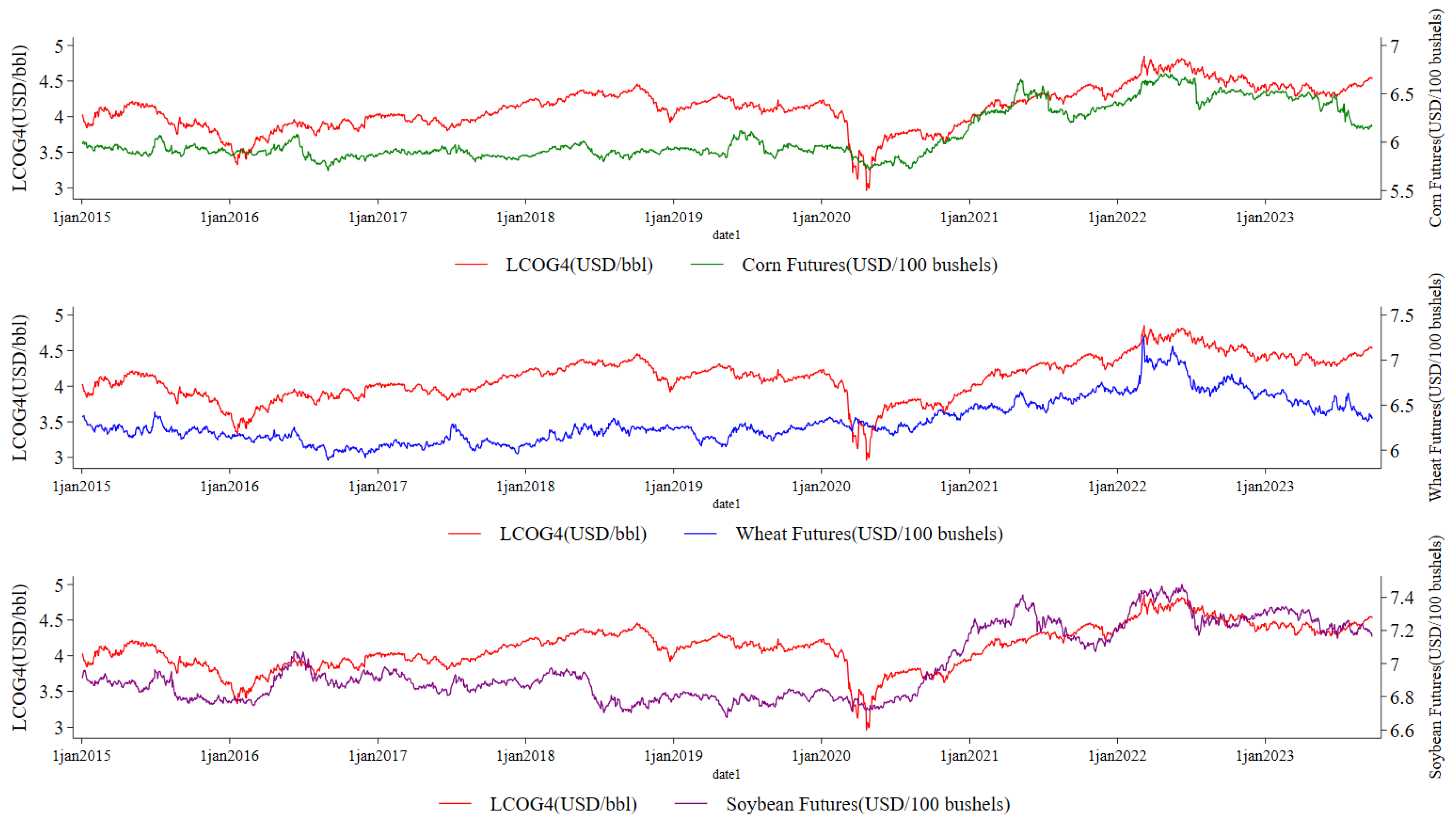
First, the stationarity of each time series was analyzed, and the logarithmic differences of each series were then taken to achieve stationary time series, followed by the construction of cointegration relationships between the markets. The logarithms and differenced results of crude oil and grain futures prices were tested using the ADF and PP tests, respectively. As shown in

Table 2. Variable ADF test results.

Variable	Test Type (C,T,K)	ADF Test t-Statistic	PP Statistic	Conclusion
${LOF}_t$	(C,T,1)	−1.855	−1.909	Non-stationary
${LCF}_t$	(C,T,1)	−1.500	−1.479	Non-stationary
${LWF}_t$	(C,T,1)	−1.944	−1.956	Non-stationary
${LSF}_t$	(C,T,1)	−1.314	−1.262	Non-stationary
$R_{LOF}\left(T\right)$	(C,0,1)	−46.348 ***	−46.350 ***	Stationary
$R_{LCF}\left(T\right)$	(C,0,1)	−46.649 ***	−46.655 ***	Stationary
$R_{LWF}\left(T\right)$	(C,0,1)	−44.911 ***	−44.871 ***	Stationary
$R_{LSF}\left(T\right)$	(C,0,1)	−36.572 ***	−36.623 ***	Stationary

Note: *** denote significance at the 1% levels.

, the test results for the original time series indicate non-stationary time series. The test results for the log-differenced return series reject the null hypothesis at the 1% significance level, indicating that the log-differenced series are stationary. Therefore, crude oil–corn, crude oil–soybean, and crude oil–wheat are all first-order integrated time series (I(1) process), fulfilling the precondition for the next step of testing cointegration relationships.

Building on this, to further examine the information share variations between crude oil futures and the three grain futures, it is necessary to first verify both their long-term and significant short-term interactions. As cointegration is a prerequisite for the information share model, the Engle–Granger ADF (EG-ADF) method (Engle and Granger, 1987) and the vector error correction model (ECM) were used to test the long-term and significant short-term interactions between crude oil futures and the three grain spot markets. As shown in

Table 3. Cointegration analysis of crude oil futures and grain futures prices.

Panel A: EG-ADF Test for Long-Run Cointegration Relationships
Test Category	Test Type (C,T,K)	ADF Test t-Statistic	Conclusion
${(LOF}_t,{LCF}_t)$	$(\mathrm{0,0},1)$	${-2.67}^{ \ast \ast \ast }$	Stationary
$({LOF}_t,{LWF}_t)$	$(\mathrm{0,0},1)$	${-2.85}^{ \ast \ast \ast }$	Stationary
${(LOF}_t,{LSF}_t)$	$(\mathrm{0,0},1)$	${-2.85}^{ \ast \ast \ast }$	Stationary
Panel B: ECM Test for Short-Term Interactions
Test Category	Test Type (C,T,K)	ADF Test t-Statistic	Conclusion
${(LOF}_t,{LCF}_t)$	$(\mathrm{0,0},1)$	${-46.49}^{ \ast \ast \ast }$	Stationary
$({LOF}_t,{LWF}_t)$	$(\mathrm{0,0},1)$	${-45.08 }^{\ast \ast \ast }$	Stationary
${(LOF}_t,{LSF}_t)$	$(\mathrm{0,0},1)$	${-47.52 }^{\ast \ast \ast }$	Stationary

Note: *** denote significance at the 1% levels.

, the ADF test results for long-term cointegration between crude oil futures and the three grain futures prices in Table 3 Panel A are all significant. Therefore, it can be concluded that a long-term cointegration relationship exists between crude oil futures and grain futures prices. The ECM test results in Table 3 Panel B are also significant, further indicating the existence of a short-term cointegration relationship between crude oil futures and spot markets. In summary, these results suggest that there are both long-term and significant short-term interactions between the crude oil market and the three international grain futures markets.

5.2. Information Share Test Results

From the above cointegration test results, it is evident that a cointegration relationship exists between crude oil futures and international grain futures prices. Therefore, based on this, the information share model was applied to calculate the information share of crude oil futures in price discovery for grain futures. As shown in

Table 4. Information share test between crude oil futures and grain futures.

Panel A: Full Sample Test
Crude Oil Futures and Corn Futures ${(\mathit{L}\mathit{O}\mathit{F}}_{\mathit{t}},{\mathit{L}\mathit{C}\mathit{F}}_{\mathit{t}})$				Crude Oil Futures and Wheat Futures ${(\mathit{L}\mathit{O}\mathit{F}}_{\mathit{t}},{\mathit{L}\mathit{W}\mathit{F}}_{\mathit{t}})$				Crude Oil Futures and Soybean Futures ${(\mathit{L}\mathit{O}\mathit{F}}_{\mathit{t}},{\mathit{L}\mathit{S}\mathit{F}}_{\mathit{t}})$
${LOF}_t$		${LCF}_t$		${LOF}_t$		${LWF}_t$		${LOF}_t$		${LSF}_t$
0.9979		0.0021		0.6775		0.3225		0.9495		0.0505
Panel B: Sub-Sample Test
Crude Oil Futures and Corn Futures ${(\mathit{L}\mathit{O}\mathit{F}}_{\mathit{t}},{\mathit{L}\mathit{C}\mathit{F}}_{\mathit{t}})$				Crude Oil Futures and Wheat Futures ${(\mathit{L}\mathit{O}\mathit{F}}_{\mathit{t}},{\mathit{L}\mathit{W}\mathit{F}}_{\mathit{t}})$				Crude Oil Futures and Soybean Futures ${(\mathit{L}\mathit{O}\mathit{F}}_{\mathit{t}},{\mathit{L}\mathit{S}\mathit{F}}_{\mathit{t}})$
First Stage		Second Stage		First Stage		Second Stage		First Stage		Second Stage
${LOF}_t$	${LCF}_t$	${LOF}_t$	${LCF}_t$	${LOF}_t$	${LWF}_t$	${LOF}_t$	${LWF}_t$	${LOF}_t$	${LWF}_t$	${LOF}_t$	${LWF}_t$
0.7059	0.2941	0.9745	0.0255	0.5390	0.4610	0.7629	0.2371	0.6050	0.3950	0.7417	0.2583

The first period is from January 2015 to July 2017, and the second period is from August 2017 to September 2023.

, in Panel A, the information share of crude oil futures in the crude oil–corn futures ${(\mathrm{L}\mathrm{O}\mathrm{F}}_{\mathrm{t}},{\mathrm{L}\mathrm{C}\mathrm{F}}_{\mathrm{t}})$ combination is 99.79%, while that of corn futures is 0.21%, indicating that crude oil futures have a much greater price discovery ability compared to corn futures. This means that, in the long term, the co-movement of the two markets is primarily driven by the crude oil futures market. Crude oil futures contribute 99.79% of the information for risk-free rate discovery, while corn futures contribute only 0.21%. Similarly, the analysis of crude oil–wheat futures ${(\mathrm{L}\mathrm{O}\mathrm{F}}_{\mathrm{t}},{\mathrm{L}\mathrm{W}\mathrm{F}}_{\mathrm{t}})$ and crude oil–soybean futures ${(\mathrm{L}\mathrm{O}\mathrm{F}}_{\mathrm{t}},{\mathrm{L}\mathrm{S}\mathrm{F}}_{\mathrm{t}})$ shows that the market shares of crude oil futures are 67.75% and 94.95%, respectively, both significantly higher than the corresponding grain futures market shares. These results indicate that the crude oil futures market plays a dominant role in the price discovery of the three international grain futures.

Building on Table 4 Panel A, we tested the robustness across different time spans. The full sample was divided into two phases based on the Global Economic Policy Uncertainty Index (the Global Economic Policy Uncertainty Index, adjusted for PPP, was sourced from the Economic Policy Uncertainty website (http://www.policyuncertainty.com/ (accessed on 19 December 2024)); detailed data are provided in the Appendix A). The results show that using July 2017 as the turning point, global economic uncertainty has increased steadily. The rise in the Global Economic Uncertainty Index significantly affects both international crude oil prices and futures prices [58]. Therefore, this was used as the division point to analyze changes in information share across different periods. As shown in Table 4 Panel B, the robustness test results reveal that the information share of crude oil futures in the crude oil–corn futures combination increased from 70.59% in the first phase to 97.45% in the second phase, indicating that the price dominance of crude oil futures over corn futures strengthened as global economic uncertainty increased. Similarly, in the crude oil–wheat futures combination, the information share of crude oil futures increased from 53.90% to 76.29%, and in the crude oil–soybean futures combination, it increased from 60.50% to 74.17%. This further demonstrates that the price discovery ability of crude oil futures for international grain futures has steadily improved over time. These results also validate the robustness of the information share model based on the full sample. This further supports the idea that as global economic uncertainty increases, the correlation between crude oil futures and international grain futures prices becomes stronger, and crude oil futures’ price discovery ability continues to grow.

5.3. Spillover Analysis of Raw Time Series

This study first constructed bivariate BEKK-GARCH models for crude oil futures $\left(\mathrm{L}\mathrm{O}\mathrm{F}\right)$ as well as corn ${(\mathrm{L}\mathrm{C}\mathrm{F}}_{\mathrm{t}})$, wheat ${(\mathrm{L}\mathrm{W}\mathrm{F}}_{\mathrm{t}})$, and soybean futures ${(\mathrm{L}\mathrm{S}\mathrm{F}}_{\mathrm{t}})$ to preliminarily analyze the volatility spillover in the original sequences. The model estimation results are shown in

Table 5. Estimated results of the BEKK-GARCH model for the original series.

Primary Sequence	Variable	Coeff	Std Error	T-Stat	Significant
${(LOF}_t,{LCF}_t)$	C(1,1)	0.0077	0.0008	9.9166	0.0000
	C(2,1)	−0.0022	0.0014	−1.5192	0.1287
	C(2,2)	0.0119	0.0007	17.7916	0.0000
	A(1,1)	0.4352	0.0241	18.0274	0.0000
	A(1,2)	−0.0373	0.0120	−3.1117	0.0019
	A(2,1)	−0.0101	0.0319	−0.3177	0.7507
	A(2,2)	0.6554	0.0332	19.7437	0.0000
	B(1,1)	0.8702	0.0130	67.0509	0.0000
	B(1,2)	0.0470	0.0123	3.8254	0.0001
	B(2,1)	0.0782	0.0331	2.3640	0.0181
	B(2,2)	0.5467	0.0352	15.5203	0.0000
${(LOF}_t,{LWF}_t)$	C(1,1)	0.0133	0.0009	15.1454	0.0000
	C(2,1)	0.0031	0.0017	1.7658	0.0774
	C(2,2)	0.0229	0.0005	43.0427	0.0000
	A(1,1)	0.6872	0.0287	23.9516	0.0000
	A(1,2)	−0.0148	0.0157	−0.9392	0.3476
	A(2,1)	−0.0084	0.0203	−0.4120	0.6803
	A(2,2)	0.7149	0.0292	24.4555	0.0000
	B(1,1)	0.6776	0.0214	31.6844	0.0000
	B(1,2)	0.0655	0.0207	3.1611	0.0016
	B(2,1)	0.0980	0.0402	2.4356	0.0149
	B(2,2)	0.0984	0.0318	3.0923	0.0020
${(LOF}_t,{LSF}_t)$	C(1,1)	0.0153	0.0009	17.7691	0.0000
	C(2,1)	0.0007	0.0015	0.5119	0.6087
	C(2,2)	0.0119	0.0005	23.0730	0.0000
	A(1,1)	0.7038	0.0291	24.2244	0.0000
	A(1,2)	0.0031	0.0106	0.2951	0.7679
	A(2,1)	0.0876	0.0370	2.3635	0.0181
	A(2,2)	0.7546	0.0355	21.2370	0.0000
	B(1,1)	0.6452	0.0224	28.7700	0.0000
	B(1,2)	0.0540	0.0175	3.0854	0.0020
	B(2,1)	−0.2157	0.0665	−3.2430	0.0012
	B(2,2)	−0.4366	0.0396	−11.0209	0.0000

. Volatility spillovers in the original sequences can be determined by examining the coefficients of matrices A and B. The coefficients A(1,1), A(2,2), B(1,1), and B(2,2) were tested in each pair. The results show that in all pairs, the corresponding position coefficients are significantly different from zero at the 5% level. This indicates that the ARCH and GARCH terms for each market are significant, meaning both futures markets are affected by past information shocks, with the influence showing significant volatility clustering and time-varying characteristics.

Further analysis reveals that in the estimation results for crude oil futures and corn futures, A(1,2) and B(1,2) are both significantly different from zero at the 5% level. This indicates that both the ARCH and GARCH terms of the crude oil futures market significantly impact the corn futures market price. This suggests that the corn futures market is subject to volatility clustering influenced by crude oil futures market fluctuations, and the significant B(2,1) coefficient indicates that corn futures prices will in turn affect crude oil futures price volatility. Similarly, in the estimation results for crude oil futures and wheat futures, A(1,2) and A(2,1) are not significant at the 5% level. However, B(1,2) and B(2,1) are both significant at the 5% level, indicating significant spillover effects between crude oil and wheat futures prices. This means that crude oil futures price volatility affects wheat futures prices, and wheat futures prices also influence crude oil futures prices. Lastly, in the estimation results for crude oil and soybean futures, except for A(1,2) being insignificant, A(2,1), B(2,1), and B(1,2) are all significantly different from zero at the 5% level. This confirms the existence of bidirectional spillover effects between crude oil and soybean futures.

To further examine the direction of volatility spillovers between crude oil futures and the three grain futures, a Wald test was conducted. The results, presented in

Table 6. Wald test based on the EEMD-BEKK-GARCH model.

Test Category	Null Hypothesis	Wald Test Results	p-Value	Conclusion (The Null Hypothesis)
${(LOF}_t,{LCF}_t)$	${H1}^{°}:LOF\iff {LCF}_t$	${26.001 }^{\ast \ast \ast }$	$0.0000$	Reject
	${H2}^{°}:LOF\Rightarrow {LCF}_t$	${19.648 }^{\ast \ast \ast }$	$0.0001$	Reject
	${H3}^{°}:{LCF}_t\Rightarrow {LOF}_t$	${7.379 }^{\ast \ast }$	$0.0250$	Reject
${(LOF}_t,{LWF}_t)$	${H4}^{°}:LOF\iff {LWF}_t$	${13.520}^{ \ast \ast \ast }$	$0.0090$	Reject
	${H5}^{°}:LOF\Rightarrow {LWF}_t$	${9.831 }^{\ast \ast \ast }$	$0.0073$	Reject
	${H6}^{°}:{LWF}_t\Rightarrow {LOF}_t$	${4.748 }^{\ast }$	$0.0931$	Fail to Reject
${(LOF}_t,{LSF}_t)$	${H7}^{°}:LOF\iff {LSF}_t$	${34.480}^{ \ast \ast \ast }$	$0.0000$	Reject
	${H8}^{°}:LOF\Rightarrow {LSF}_t$	${21.931 }^{\ast \ast \ast }$	$0.0000$	Reject
	${H9}^{°}:{LSF}_t\Rightarrow {LOF}_t$	${7.9504 }^{\ast \ast }$	$0.0188$	Reject

Note: ***, ** and * denote significance at the 1%, 5% and 10%, respectively. H1–H9 represent the null hypotheses (i.e., no volatility spillover in that direction), with the superscript o indicating the null hypothesis.

, use arrows to indicate the direction of spillover between the markets. For the bidirectional arrow $(\mathrm{j}\iff \mathrm{i})$, the null hypothesis is $\mathrm{A}(\mathrm{i},\mathrm{j})=\mathrm{A}(\mathrm{j},\mathrm{i})=\mathrm{B}(\mathrm{i},\mathrm{j})=\mathrm{B}(\mathrm{j},\mathrm{i})=0$; if the null hypothesis is rejected, it indicates the presence of volatility spillovers between the markets. The null hypothesis for one-way arrows is $(\mathrm{j}\Rightarrow \mathrm{i}):\mathrm{A}(\mathrm{j},\mathrm{i})=\mathrm{B}(\mathrm{j},\mathrm{i})=0$. If the null hypothesis is rejected, it indicates a one-way volatility spillover from market j to market i. According to the Table 6, the Wald tests of ${\mathrm{H}1}^{°},{\mathrm{H}4}^{°},{\mathrm{H}7}^{°}$ uniformly reject the null hypothesis, indicating that the matrix elements are significantly non-zero. This suggests the presence of volatility spillover effects between crude oil futures and the three types of grain futures. Further analysis of hypotheses ${\mathrm{H}2}^{°}$ and ${\mathrm{H}3}^{°}$ in the combination of crude oil futures and corn futures reveals that both reject the original hypotheses at the 5% level of significance, suggesting that there is a two-way volatility spillover between the two. Testing results of hypotheses ${\mathrm{H}5}^{°}$ and ${\mathrm{H}6}^{°}$ for the combination of crude oil futures and wheat futures show that H5 is significant at the 5% level, while H6 is significant only at the 10% level. This indicates that the volatility spillover from crude oil futures to wheat futures is unidirectional. Testing results of hypotheses ${\mathrm{H}8}^{°}$ and ${\mathrm{H}9}^{°}$ for the combination of crude oil futures and soybean futures reveal that both hypotheses are significant at the 5% level. This finding indicates a bidirectional volatility spillover between crude oil futures and soybean futures.

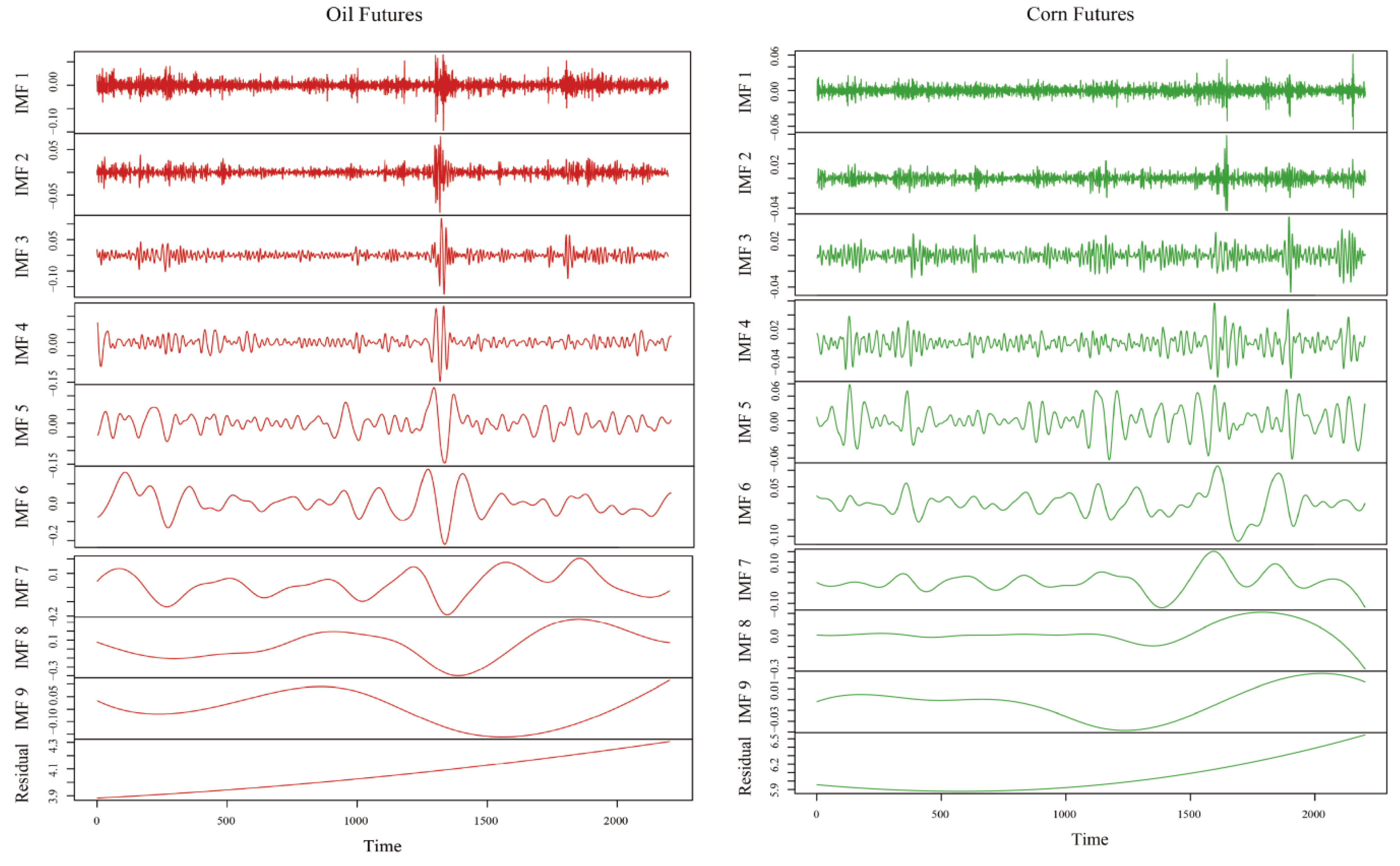
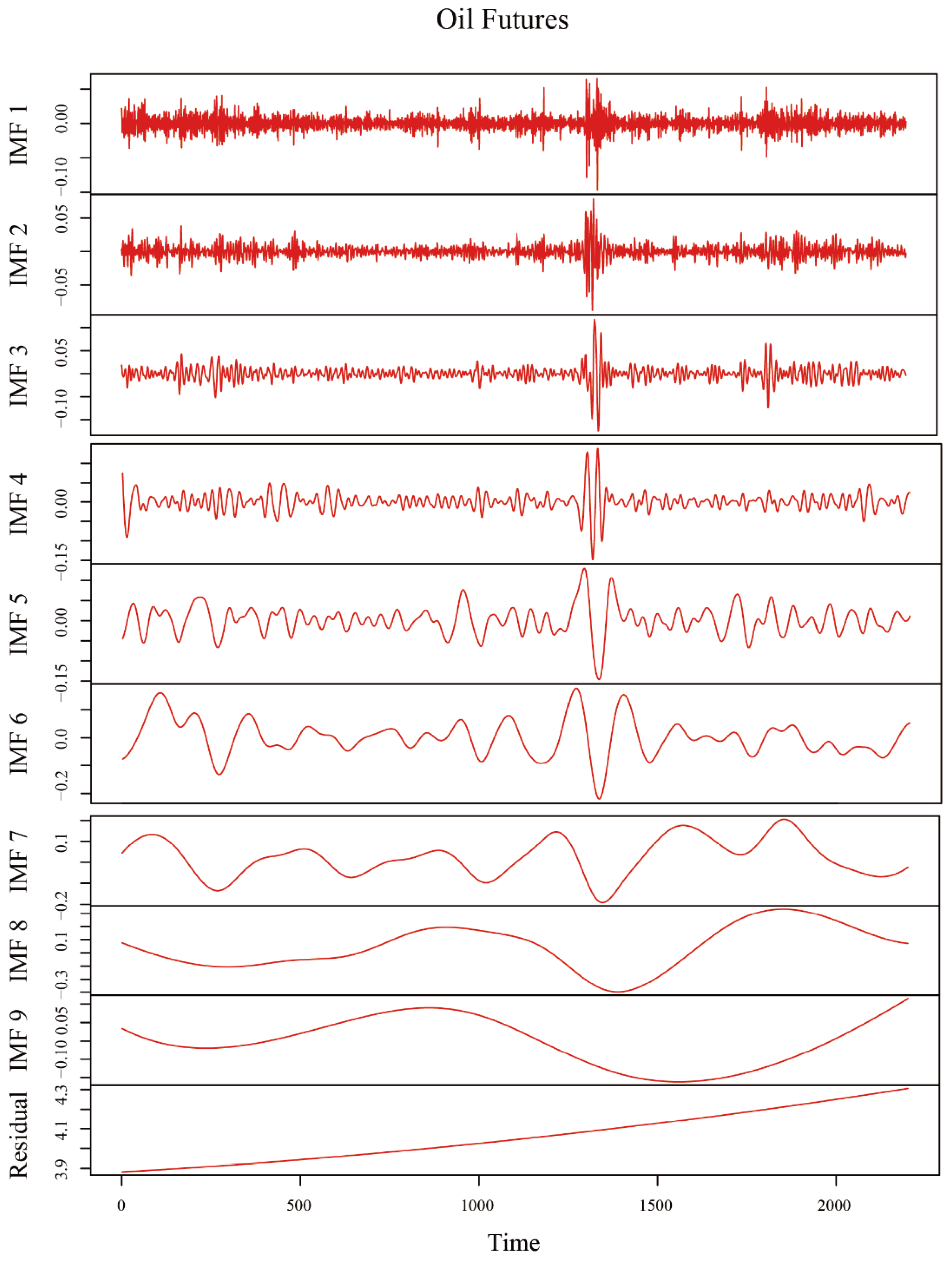
5.4. Volatility Spillover Analysis Based on the EEMD-BEKK-GARCH Model

Based on the results of the above analysis, this study further used the EEMD method to decompose the crude oil futures and the three international grain futures prices with the time span of 2015–2023. The trend term, low-frequency term, and high-frequency term were then constructed according to the frequency distribution, which were used to represent the long-term trend, the medium-term impact of emergencies, and the volatility characteristics caused by the short-term speculation. The volatility spillover between futures markets under different cycles was analyzed through the BEKK-GARCH model. The volatility spillover between futures markets under different cycles was analyzed, and the results are shown in

Table 7. Wald test of the EEMD-BEKK-GARCH model.

Decomposition Sequence	Null Hypothesis	Wald Test Results	p-Value	Conclusion (The Null Hypothesis)
High-frequency component	${\mathrm{H}1}^{\mathrm{h}}:{\mathrm{L}\mathrm{O}\mathrm{F}}_{\mathrm{t}}\iff {\mathrm{L}\mathrm{C}\mathrm{F}}_{\mathrm{t}}$	${35.1621 }^{\ast \ast \ast }$	$0.0000$	Rejection
	${\mathrm{H}2}^{\mathrm{h}}:{\mathrm{L}\mathrm{O}\mathrm{F}}_{\mathrm{t}}\Rightarrow {\mathrm{L}\mathrm{C}\mathrm{F}}_{\mathrm{t}}$	${17.4729 }^{\ast \ast \ast }$	$0.0002$	Rejection
	${\mathrm{H}3}^{\mathrm{h}}:{\mathrm{L}\mathrm{C}\mathrm{F}}_{\mathrm{t}}\Rightarrow {\mathrm{L}\mathrm{O}\mathrm{F}}_{\mathrm{t}}$	${16.8121 }^{\ast \ast \ast }$	$0.0002$	Rejection
	${\mathrm{H}4}^{\mathrm{h}}:{\mathrm{L}\mathrm{O}\mathrm{F}}_{\mathrm{t}}\iff {\mathrm{L}\mathrm{W}\mathrm{F}}_{\mathrm{t}}$	${17.5336 }^{\ast \ast }$	$0.0015$	Rejection
	${\mathrm{H}5}^{\mathrm{h}}:{\mathrm{L}\mathrm{O}\mathrm{F}}_{\mathrm{t}}\Rightarrow {\mathrm{L}\mathrm{W}\mathrm{F}}_{\mathrm{t}}$	${16.1434}^{ \ast \ast \ast }$	$0.0003$	Rejection
	${\mathrm{H}6}^{\mathrm{h}}:{\mathrm{L}\mathrm{W}\mathrm{F}}_{\mathrm{t}}\Rightarrow {\mathrm{L}\mathrm{O}\mathrm{F}}_{\mathrm{t}}$	$2.6829$	$0.2615$	Fail to reject
	${\mathrm{H}7}^{\mathrm{h}}:{\mathrm{L}\mathrm{O}\mathrm{F}}_{\mathrm{t}}\iff {\mathrm{L}\mathrm{S}\mathrm{F}}_{\mathrm{t}}$	${21.9783 }^{\ast \ast \ast }$	$0.0002$	Rejection
	${\mathrm{H}8}^{\mathrm{h}}:{\mathrm{L}\mathrm{O}\mathrm{F}}_{\mathrm{t}}\Rightarrow {\mathrm{L}\mathrm{S}\mathrm{F}}_{\mathrm{t}}$	${11.3213 }^{\ast \ast \ast }$	$0.0035$	Rejection
	${\mathrm{H}9}^{\mathrm{h}}:{\mathrm{L}\mathrm{S}\mathrm{F}}_{\mathrm{t}}\Rightarrow {\mathrm{L}\mathrm{O}\mathrm{F}}_{\mathrm{t}}$	${12.3741 }^{\ast \ast \ast }$	$0.0021$	Rejection
Low-frequency component	${\mathrm{H}1}^{\mathrm{l}}:{\mathrm{L}\mathrm{O}\mathrm{F}}_{\mathrm{t}}\iff {\mathrm{L}\mathrm{C}\mathrm{F}}_{\mathrm{t}}$	${125.1957 }^{\ast \ast \ast }$	$0.0000$	Rejection
	${\mathrm{H}2}^{\mathrm{l}}:{\mathrm{L}\mathrm{O}\mathrm{F}}_{\mathrm{t}}\Rightarrow {\mathrm{L}\mathrm{C}\mathrm{F}}_{\mathrm{t}}$	${92.7227 }^{\ast \ast \ast }$	$0.0000$	Rejection
	${\mathrm{H}3}^{\mathrm{l}}:{\mathrm{L}\mathrm{S}\mathrm{F}}_{\mathrm{t}}\Rightarrow {\mathrm{L}\mathrm{O}\mathrm{F}}_{\mathrm{t}}$	${69.7027 }^{\ast \ast \ast }$	$0.0000$	Rejection
	${\mathrm{H}4}^{\mathrm{l}}:{\mathrm{L}\mathrm{O}\mathrm{F}}_{\mathrm{t}}\iff {\mathrm{L}\mathrm{W}\mathrm{F}}_{\mathrm{t}}$	${159.6631 }^{\ast \ast \ast }$	$0.0000$	Rejection
	${\mathrm{H}5}^{\mathrm{l}}:{\mathrm{L}\mathrm{O}\mathrm{F}}_{\mathrm{t}}\Rightarrow {\mathrm{L}\mathrm{W}\mathrm{F}}_{\mathrm{t}}$	${56.1332 }^{\ast \ast \ast }$	$0.0000$	Rejection
	${\mathrm{H}6}^{\mathrm{l}}:{\mathrm{L}\mathrm{W}\mathrm{F}}_{\mathrm{t}}\Rightarrow {\mathrm{L}\mathrm{O}\mathrm{F}}_{\mathrm{t}}$	${57.9586 }^{\ast \ast \ast }$	$0.0000$	Rejection
	${\mathrm{H}7}^{\mathrm{l}}:{\mathrm{L}\mathrm{O}\mathrm{F}}_{\mathrm{t}}\iff {\mathrm{L}\mathrm{S}\mathrm{F}}_{\mathrm{t}}$	${614.2301 }^{\ast \ast \ast }$	$0.0000$	Rejection
	${\mathrm{H}8}^{\mathrm{l}}:{\mathrm{L}\mathrm{O}\mathrm{F}}_{\mathrm{t}}\Rightarrow {\mathrm{L}\mathrm{S}\mathrm{F}}_{\mathrm{t}}$	${216.4190 }^{\ast \ast \ast }$	$0.0000$	Rejection
	${\mathrm{H}9}^{\mathrm{l}}:{\mathrm{L}\mathrm{S}\mathrm{F}}_{\mathrm{t}}\Rightarrow {\mathrm{L}\mathrm{O}\mathrm{F}}_{\mathrm{t}}$	${338.1867 }^{\ast \ast \ast }$	$0.0000$	Rejection
Trend component	${\mathrm{H}1}^{\mathrm{r}}:{\mathrm{L}\mathrm{O}\mathrm{F}}_{\mathrm{t}}\iff {\mathrm{L}\mathrm{C}\mathrm{F}}_{\mathrm{t}}$	${26.3624 }^{\ast \ast \ast }$	$0.0010$	Rejection
	${\mathrm{H}2}^{\mathrm{r}}:{\mathrm{L}\mathrm{O}\mathrm{F}}_{\mathrm{t}}\Rightarrow {\mathrm{L}\mathrm{C}\mathrm{F}}_{\mathrm{t}}$	${11.2080 }^{\ast \ast \ast }$	$0.0001$	Rejection
	${\mathrm{H}3}^{\mathrm{r}}:{\mathrm{L}\mathrm{C}\mathrm{F}}_{\mathrm{t}}\Rightarrow {\mathrm{L}\mathrm{O}\mathrm{F}}_{\mathrm{t}}$	${19.8704 }^{\ast \ast \ast }$	$0.8105$	Fail to reject
	${\mathrm{H}4}^{\mathrm{r}}:{\mathrm{L}\mathrm{O}\mathrm{F}}_{\mathrm{t}}\iff {\mathrm{L}\mathrm{W}\mathrm{F}}_{\mathrm{t}}$	${21.4194 }^{\ast \ast \ast }$	$0.0000$	Rejection
	${\mathrm{H}5}^{\mathrm{r}}:{\mathrm{L}\mathrm{O}\mathrm{F}}_{\mathrm{t}}\Rightarrow {\mathrm{L}\mathrm{W}\mathrm{F}}_{\mathrm{t}}$	${14.5767 }^{\ast \ast \ast }$	$0.0000$	Rejection
	${\mathrm{H}6}^{\mathrm{r}}:{\mathrm{L}\mathrm{W}\mathrm{F}}_{\mathrm{t}}\Rightarrow {\mathrm{L}\mathrm{O}\mathrm{F}}_{\mathrm{t}}$	${15.0379 }^{\ast \ast \ast }$	$0.3600$	Fail to reject
	${\mathrm{H}7}^{\mathrm{r}}:{\mathrm{L}\mathrm{O}\mathrm{F}}_{\mathrm{t}}\iff {\mathrm{L}\mathrm{S}\mathrm{F}}_{\mathrm{t}}$	${39.1003 }^{\ast \ast \ast }$	$0.0218$	Rejection
	${\mathrm{H}8}^{\mathrm{r}}:{\mathrm{L}\mathrm{O}\mathrm{F}}_{\mathrm{t}}\Rightarrow {\mathrm{L}\mathrm{S}\mathrm{F}}_{\mathrm{t}}$	${9.3891 }^{\ast \ast \ast }$	$0.0038$	Rejection
	${\mathrm{H}9}^{\mathrm{r}}:{\mathrm{L}\mathrm{S}\mathrm{F}}_{\mathrm{t}}\Rightarrow {\mathrm{L}\mathrm{O}\mathrm{F}}_{\mathrm{t}}$	${19.3109 }^{\ast \ast \ast }$	$0.9227$	Fail to reject

Note: *** and ** denote significance at the 1% and 5% levels, respectively. Arrows represent the direction of volatility spillovers, with ⇔ indicating two-way spillovers between both markets and ⇒ representing a one-way volatility spillover from the left market to the right market. H1–H9 represent the null hypotheses (i.e., there is no volatility spillover in that direction), with superscripts r, l, and h denoting the trend, low-frequency, and high-frequency terms, respectively.

.

Table 7 reveals that, with regard to the high-frequency terms, all hypotheses except ${\mathrm{H}6}^{\mathrm{h}}$ reject the null hypothesis. Specifically, in short-term futures trading, there is a two-way spillover effect between crude oil futures and both corn and soybean futures. However, the test results for wheat futures indicate a unidirectional spillover effect from crude oil futures to wheat futures. This finding is corroborated by the analysis of the original series, which confirms the presence of a unidirectional spillover from crude oil futures to wheat futures. In the low-frequency term analyses, all tests (${\mathrm{H}1}^{\mathrm{l}}-{\mathrm{H}9}^{\mathrm{l}}$) reject the null hypothesis, indicating significant two-way spillover effects between crude oil futures and the three grain futures prices in medium-term trading. In the trend term analysis, hypotheses ${\mathrm{H}1}^{\mathrm{r}},{\mathrm{H}6}^{\mathrm{r}}$, and ${\mathrm{H}9}^{\mathrm{r}}$ fail to reject the null hypothesis, while the remaining hypotheses are significant at the 5% level. This indicates one-way volatility spillovers from the crude oil futures market to the three grain futures markets in the long-term trading trend.

It can be observed that the volatility spillover results between the EEMD and the original sequence are largely consistent, though some differences remain. In terms of similarities, the high-frequency volatility spillover analysis shows bidirectional spillovers between crude oil futures and both corn and soybean futures, while a unidirectional spillover effect is observed between crude oil and wheat futures. This result is largely consistent with the spillover analysis of the original sequence. The differences lie in two main aspects. First, in the low-frequency component, the test results for crude oil and all three grain futures reject the null hypothesis, indicating bidirectional spillovers during long-term volatility, which contrasts with the unidirectional spillover from crude oil to wheat futures in the original sequence. As the low-frequency component primarily reflects medium-term effects, this result also suggests differences in the impact of factors such as Federal Reserve interest rate hikes, the COVID-19 pandemic, and related policies on the relationship between crude oil and grain futures. Second, in the trend component analysis, the transmission effect of the three grain futures on crude oil futures is insignificant, indicating that in terms of long-term volatility spillovers, the crude oil futures market has a unidirectional influence on the grain futures markets.

6. Conclusions and Policy Recommendations

This study investigated cross-market and cross-cycle volatility patterns among crude oil, corn, wheat, and soybean futures markets. Using daily futures trading data from January 2015 to September 2023, the information share model was applied to study the price discovery ability of crude oil futures relative to the three grain futures under long-term cointegration conditions. Furthermore, the EEMD model was used to capture the characteristics of each time series over long-, medium-, and short-term cycles, and in combination with the BEKK-GARCH model, the spillover effects between crude oil futures and the three grain futures across different cycle lengths were examined. The results are as follows. First, the information share test indicates that crude oil futures have a significant advantage in information share compared to grain futures. This implies that in the long term, crude oil futures play a dominant role in influencing grain futures price movements. Second, in terms of short-term volatility spillovers, all but wheat futures exhibit bidirectional spillovers, with wheat futures showing unidirectional spillovers. For medium-term volatility spillovers, crude oil and grain futures show bidirectional spillovers, whereas for long-term volatility spillovers, crude oil futures exhibit unidirectional spillovers affecting grain futures prices.

Based on the conclusions of this paper, the following recommendations are provided. Futures market investors should fully consider the inter-temporal information shocks across markets when making investment decisions and constructing portfolios. In long-term investments, it is crucial to closely monitor the trends of crude oil futures, the US Dollar Index, and other financial indices under global macroeconomic policy adjustments to anchor long-term trends in grain futures. Short-term contract holders should focus on diversifying and hedging risk across multiple products to mitigate the negative effects of speculation and market sentiment on short-term futures price movements.

For regulatory authorities, it is essential to strengthen institutional frameworks and develop multi-market and multi-agency regulatory systems. This would enhance macro-prudential supervision, reduce cross-market contagion between financial markets, and ensure the stability of the financial system. Additionally, improving multi-cycle risk warning models and establishing long-, medium-, and short-term risk monitoring platforms will enhance cross-cycle regulation and reduce the occurrence of systemic market risks.