Abstract
One of the primary factors in the hydrological cycle is reference evapotranspiration (ET0). The prediction of ET0 is crucial to manage irrigation water in agriculture under climate change; however, little research has been conducted on the trends of ET0 changes in Shandong Province. In this study, to estimate ET0 in the entire Shandong Province, 245 sites were chosen, and the monthly ET0 values during 1901–2020 were computed using the Hargreaves–Samani formula. A deep learning model, termed SAO-CNN-BiGRU-Attention, was utilized to forecast the monthly ET0 during 2021–2100, and the predictions were compared to two CMIP6 climate scenarios, SSP2-4.5 and SSP5-8.5. The hierarchical clustering results revealed that Shandong Province encompassed three homogeneous regions. The ET0 values of Clusters H1 and H2, which were situated in inland regions and major agricultural areas, were the highest. The SAO-CNN-BiGRU-Attention and SSP5-8.5 forecasting results generally displayed a monotonically growing trend during the forecast period in the three regions; however, the SAO-CNN-BiGRU-Attention model displayed a declining tendency at a few points. According to the SAO-CNN-BiGRU-Attention and SSP5-8.5 results, during 2091–2100, H1, H2, and H3 will reach their peaks; the SSP2-4.5 results show that H1, H2, and H3 will peak in 2031–2040. At the end of the forecast period, for Clusters H1, H2, and H3, the prediction rate of SAO-CNN-BiGRU-Attention increased by 1.31, 1.56%, and 1.80%, respectively, whereas SSP2-4.5’s prediction rate increased by 0.31%, 0.95%, and 1.57%, respectively, and SSP5-8.5’s prediction rate increased by 10.88%, 10.76%, and 10.69%, respectively. The prediction results of SAO-CNN-BiGRU-Attention were similar to those of SSP2-4.5 (R2 > 0.96). The SAO-CNN-BiGRU-Attention deep learning model can be used to forecast future ET0.
1. Introduction
One of the main features of the hydrological cycle is evapotranspiration [1]. Therefore, the precise determination of reference evapotranspiration (ET0) is crucial for water resource management and optimal irrigation scheduling [2]. Water circulation patterns have undergone considerable changes as a result of global climate change [3,4], marked by low rainfalls and high temperatures [5]. In the same vein, ET0 has also been severely impacted [6]. Using meteorological data, an analysis of the steaming effect and ET0 distribution in the Senegal River Basin revealed that, between 1984 and 2017, 32% of the basin’s ET0 area expanded significantly [7]. The Loess Plateau region, upstream of the Yellow River, underwent a progressive increase in temperature between 2001 and 2020, and this coincided with a steady increase in ET0 [8]. Climate change is the primary cause of changes in the diverse processes of the Yellow River source area, and research revealed that the climate will become more humid and warm in this area and that ET0 will increase by 10.4% in the Maqu secondary basin [9]. Four ecosystems (forest, shrub, farmland, and grassland) were simulated using CMIP6, and the results showed that ET0 gradually increased as the CO2 concentration increased [10].
The Penman–Monteith (PM) [11,12,13] and Hargreaves–Samani (HS) [14,15] formulas, recommended by the Food and Agriculture Organization of the United Nations, are the primary methods used to determine ET0. In a previous study using the HS formula, ET0 analysis in Hami, China, showed increasing trends from 1991 to 2020, except for winter [16]. When calculating ET0 in the arid regions of central–north Mexico, the HS model yielded more accurate results than the PM model [17]. Compared to the PM formulas, HS formulas only require solar radiation and maximum and minimum temperature. However, the empirical coefficient’s value determines how accurate the ET0 estimate is. In China, the accuracy of the modified HS formula is higher than the original HS formula [18], and in different climate zones, the results of the modified HS formula are fairly close to those of the PM formula.
Many weather characteristics have been included in the original computing formulas; however, data collection is frequently challenging, and these formulas are not particularly suitable for future ET0 prediction. In this regard, another method has emerged with the advent of deep learning that does not require many challenging physical parameters [19]. In recent years, deep learning has been extensively employed in hydrological models used for ET0 estimation [20,21]. Recurrent Neural Networks (RNNs), Long Short-Term Memory (LSTM), and Bidirectional LSTM were used on Prince Edward Island, Canada, to estimate ET0. The results revealed that LSTM and Bidirectional LSTM were the most appropriate methods to accurately estimate ET0, achieving results at the majority of sites. The accuracy of LSTM and Bidirectional LSTM were not significantly different [22]. The effects of Random Forest (RF), Gradient-Boosting Machine (GBM), Generalized Linear Model (GLM), and Deep Learning–Multilayer Perceptron (DL) in Punjab Province, India, were investigated using the H2O model framework. The DL model demonstrated superior performance [23].
Convolutional Neural Networks (CNNs) are also frequently utilized for hydrological forecasts. CNNs have a great ability to capture the local features of the data [24], and time sequence challenges can be effectively addressed using CNNs [25]. Compared to the original machine learning model, the forecast’s accuracy can be significantly increased by incorporating the CNN model [26]. The benefit of the Bidirectional Gated Recurrent Unit (BiGRU) is that it can solve gradient explosions, since the GRU forecasts successful time sequence performance [27]. The BiGRU can effectively improve the accuracy of the prediction of evapotranspiration [28]. The attention mechanism allows for the selection of prominent characteristics from data based on the relationships between the data [29]. In recent years, CNN-BiGRU-Attention has been widely used in time series prediction, and its performance is superior to that of traditional models [30]; however, there has been relatively little research conducted utilizing the CNN-BiGRU-Attention model for forecasting ET0 in the future.
The meticulous selection of hyperparameters significantly influences the accuracy of predictive models [31]. In this research, the snow ablation optimizer algorithm was used for hyperparameter optimization. The primary goal of the snow ablation optimizer algorithm is to mimic the behavior of snow melting and sublimation to balance space exploration and development and avoid premature convergence. Here, 22 CEC2020 real-world constrained optimization problems and 29 typical CEC2017 unconstrained benchmarks were used, including 7 synthesis and design problems and 15 mechanical engineering problems. The SAO algorithm was applied to extract the key parameters in photovoltaic systems, and the simulation results demonstrate that the SAO algorithm is a promising technology, as it outperforms other complex algorithms [32].
China’s Shandong Province is a major winter wheat region [33,34]. In 2021, the largest winter crop in the area was winter wheat, with a planting area of 3,949,353.08 hm2 [35]. However, there was a shortage of fresh water for irrigation [36]. In 2018, the province’s total water consumption was 21,266 billion cubic meters, with agriculture accounting for 62.8% (13,346 billion cubic meters). Irrigation used 11,468 billion cubic meters, accounting for 85.9% of the water consumption in agriculture. The share of the region in terms of per capita water resources was only one-sixth of the national rate, accounting for 4.0% of the world’s share [37]. Therefore, the precise estimation of ET0 is crucial for freshwater conservation.
The change in Shandong Province’s ET0 from 1980 to 2019 was 1070.5 mm, and the ET0 percentages in spring, summer, autumn, and winter were 29%, 40%, 21%, and 10% of the total ET0, respectively [34]. Previous studies generally concentrated on analyzing changes in the spatial–temporal distribution and the sensitivity of controlling variables, [38]; however, there has been less research on the trajectory of ET0 changes in Shandong Province. Previous studies have mostly focused on space–time distribution and the factors affecting ET0 estimation. As a result of factors such as human-caused global climate change [39,40], agricultural water scarcity will likely be an increasing challenge in the future [37]. Therefore, it is crucial to research the future changing trends of ET0 to preserve irrigation water. This article provides a reference for the preservation of freshwater resources and advancing agriculture using future climate data, determined using CMIP6 and the deep learning model SAO-CNN-BiGRU-Attention to estimate ET0 trends in Shandong Province, China. A Mann–Kendall test was then used to verify the trends.
2. Materials and Methods
2.1. Study Area Description
Shandong Province is situated in China’s eastern region (34°22.9′–38°24.01′ N, 114°47.5′–122°42.3′ E). The east of Shandong Province has rolling hills, while its southwest and northwest areas are low-lying and flat. The middle region of the province is home to numerous mountains. The Shandong Peninsula lies to the east, the North China Plain lies to the west and north, and the majority of the topography comprises mountains and hills [41].
Shandong Province has a warm temperate monsoon climate, with scorching summers and rainy winters that are dry and frigid. The average yearly temperature ranges from 11 to 14 °C, with a larger temperature difference between east and west than between north and south. Precipitation decreases from the southeast to the northwest, with an annual total of 550 to 950 mm. The average amount of annual light is between 2290 and 2890 h, and crops require constricted heat conditions twice a year [35].
The General Bathymetric Chart of the Oceans was used to collect DEM data, as shown in Figure 1. In total, 245 points were selected to represent the entire region. The Aerospace Information Research Institute, Chinese Academy of Sciences, provided the land cover data [42], as seen in Figure 2.
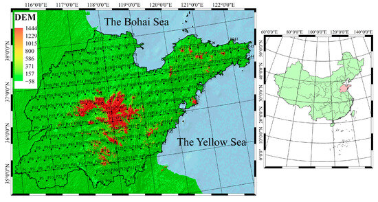
Figure 1.
DEM data and the analyzed points in Shandong Province.
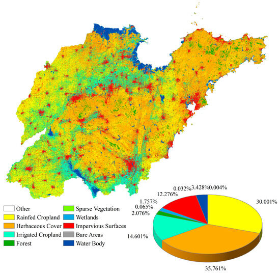
Figure 2.
Land cover of Shandong Province.
2.2. Dataset
The 1 km monthly maximum [43] and minimum temperature dataset [44] was derived from the National Tibetan Plateau/Third Pole Environment Data Center, with a historical range of 1901 to 2020 [45,46,47,48]. The historical extraterrestrial radiation (Ra) was calculated as follows:
where Gsc is the solar constant, dr is the inverse relative distance of Earth to the Sun, ωs is the sunset hour angle, φ is the latitude, and δ is solar declination [1].
A modified Hargreaves–Samani formula was utilized to determine ET0 as follows:
where α = 0.415, β = 0.049, Tmax is the monthly maximum temperature, and Tmin is the monthly minimum temperature [18].
The shared socioeconomic pathway (SSP) was used in CMIP6, meaning that emissions, land use scenarios, pattern parameters, and physical processes were the primary inputs. SSP2-4.5 and SSP5-8.5 were also used, with SSP2-4.5 indicating intermediate and SSP5-8.5 indicating high levels of greenhouse gas emissions [49]. The global climate model (GCM) was MRI-ESM2-0 with a future time range of 2021 to 2100. This dataset was used after adjustment.
2.3. Methods
2.3.1. Technical Route
Based on the investigation, Figure 3 displays the technical route and flow diagram of the SAO-CNN-BiGRU-Attention model, and Table 1 provides the upper and lower bounds of the hyperparameters. The learning rate, L2 regularization parameters, and number of hidden layer nodes of the CNN-BiGRU-Attention model were optimized using the SAO algorithm; these values are hard to choose based only on experience and have a significant influence on model performance. Additional hyperparameters were chosen in accordance with experience, with the Supplementary Materials containing the precise parameters. In the model, a 2D CNN model is employed to enhance its performance. In this research, time was used as a label, and the historical data were used as a training set for the time series forecasting of ET0. The dataset was split into training and testing sets at a ratio of 60%:40%. Initially, we intended to include other basic models, but the preliminary results showed that their performance was worse than that of SAO-CNN-BiGRU-Attention. More details can be found in the Supplementary Materials.
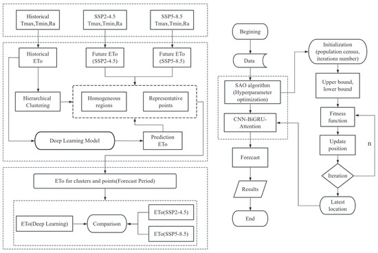
Figure 3.
Technical route and flow diagram of SAO-CNN-BiGRU-Attention model.

Table 1.
Lower and upper bounds of hyperparameters.
2.3.2. Cluster Procedure
In hierarchical clustering analysis, a layered stacked cluster tree is generated by comparing several data points. The procedure is as follows. First, each sample is individually generated at the start of the clustering class formation; next, a specific method is chosen to determine the degree of similarity between all samples. The most similar samples are then clustered into a small category. The degree of similarity between the small category and the remaining samples is again determined, and, lastly, similar samples are gathered into one category. This process is repeated until all samples are gathered into one category [50]. In this research, the average, maximum, and standard deviation of ET0, and the numbers of months with the ET0 reaching 0–0.6 mm/day, 0.6–1.2 mm/day, 1.2–1.8 mm/day, 1.8–2.4 mm/day, and 2.4–3.0 mm/day were used as parameters for hierarchical clustering. The parameters are displayed in Table 2.

Table 2.
ET0 statistical parameter average for each cluster, expressed in mm/day.
The Davies–Bouldin index was used for the preliminary analysis to identify the optimal k value of the clustering class in order to determine the optimal clustering number, which is expressed as follows:
where Si represents the average separation between each element and the cluster center [51]. Hierarchical clustering was carried out based on the minimum Davies–Bouldin index [52].
The Manhattan distance and the Ward linkage were used to calculate distance between two clusters. They are more influenced by the similarity of the other variables, being more robust and less affected by outliers [1]. The Manhattan distance measures the separation between two points in a space, denoted by coordinates of a(x1, x2, …, xn) and b(y1, y2, …, yn), which is determined as follows:
where k is the vector’s dimension [53].
The Ward linkage is used to calculate the distance between clusters r and s and is determined as follows:
where SSErs is the sum of the square error of total, SSEr is the sum of the square error of cluster r, and SSEs is the sum of the square error of cluster s [1].
2.3.3. Snow Ablation Optimizer (SAO) Algorithm
(1) In the initialization stage, a matrix is created using cluster modeling, as follows:
where L and U represent the lower and upper boundaries of the solution space, respectively; θ is an integer generated at random in [0, 1]; n is the number of rows; and Dim is the number of columns.
(2) In the exploration stage, possible locations are investigated, and irregular steam movements are simulated using Brownian motion, which is computed using the following formula:
where Zi(t) is the ith individual during the t-th iteration; BMi(t) is a vector including random numbers based on Gaussian distribution, denoting the Brownian motion; ⊗ is entry-wise multiplication; θ1 is a randomly generated number in [0, 1]; G(t) is the current best solution; Elite(t) is a random individual selected from a set of several elites in the swarm; is the centroid position of the whole swarm; Zsecond(t) and Zthird(t) are the second- and third-best individuals in the current population, respectively; Zc(t) is the centroid position of individuals whose fitness values rank in the top 50%; N1 is the number of leaders; and Zi(t) is the ith best leader.
(3) In the exploitation stage, the melting process of snow is simulated using the degree–day approach, and the resulting snowmelt rate, M, is expressed as follows:
where tmax is the termination criterion.
The following equation is:
where M is the snowmelt rate, and θ2 represents a randomly generated number in [−1, 1].
2.3.4. CNN, BiGRU, and SE Attention
During deep neural network training, the input distribution of each layer continues to be updated with weight parameters, resulting in slow convergence speed. Thus, to improve the performance and stability of Convolutional Neural Networks, after a Batch Normalization Layer is added to a Convolutional Layer, it normalizes each small batch of data to increase the stability of input distribution and boost the effectiveness and precision of training. A Max-Pooling Layer, which is added to the previous two layers, helps to better process the model’s time sequence data and improves robustness to noise and fluctuations. Its functions include decreased sampling, feature extraction, translation invariability, and data backbone. The CNN model is established as follows:
where Yi, j is the output feature mapping value; Wm, n is the m × n weight matrix of the convolution kernel; Xi+m, j+n is the input feature mapping value; b is the bias vector; ⊗ is matrix multiplication operation; f is the nonlinear activation function; and σ is the activation function ReLU [54].
The same input sequence was connected to forward and back units using BiGRU, and the two networks’ hidden layers were then connected to the output layer for prediction. The two hidden layers received the same input continuously but in different directions, thus enhancing the extraction of forward and backward time sequence features. These principles can be expressed as follows:
where the GRU function is the nonlinear transformation of the input time sequence data; xt is the input at time t; ht+ is the output of the Forward Hidden State at time t; ht− is the output of the Backward Hidden State at time t; wt is the weight corresponding to the Forward Hidden State at time t; vt is the weight corresponding to the Backward Hidden State at time t; and bt is the Bias corresponding to the two hidden states of BiGRU at time t [55].
In a representative channel attention mechanism, called SE Attention, the input feature I of channel C is first compressed by Squeeze Operation Fsq. Then, it is transported to the Fully Connected Layer of the Excitation Operation Fex, and the activation function sigmoid generates Feature Channel Weights. Lastly, the Reweight operation completes the process of recalling raw features and obtaining attention-based feature extraction results. The principles can be expressed as follows:
where Fsq and Fscale are the global average pooling and weighting, respectively; Fex indicates processing through two fully connected and activation functions; Uc(i, j) represents the feature value of the channel C of the position (i, j); H and W represent the height and width of the feature, respectively; W1 and W2 represent the parameter matrix; σ represents the activation function sigmoid; and Uc and Sc represent the two-dimensional matrix and weights, respectively [56].
2.4. Evaluation Criteria
Four distinct evaluation criteria were used to compare the SAO-CNN-BiGRU-Attention’s prediction with the SSP2-4.5 and SSP5-8.5 future scenarios, namely, the coefficient of determination (R2), the root-mean-square error (RMSE), the mean absolute error (MAE), and the mean absolute percentage error (MAPE) [1,19].
Here, Yoi is the value of SSP2-4.5 or SSP5-8.5 future scenario; Ypi is the SAO-CNN-BiGRU-Attention prediction value; is the average value of SSP2-4.5 or SSP5-8.5; and n is the total volume of data predicted in the time series.
3. Results
3.1. Hierarchical Clustering
Based on the Davies–Bouldin index minimum, the province can be classified into three homogeneous zones, denoted as H1, H2, and H3. Table 3 provides the Davies–Bouldin index of different k values. Figure 4 displays the partition diagram generated using the inverse distance weighting method (IDW) [57] as well as the hierarchical clustering dendrogram diagram. The analysis report includes high and low representative points using Origin 2021 for clustering. Figure 5 displays the land cover inside each cluster, and Figure 6 presents the DEM analysis results within each cluster.

Table 3.
Davies–Bouldin index of different k values; bold indicates the minimum value.
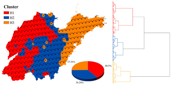
Figure 4.
Partition diagram and dendrogram diagram.
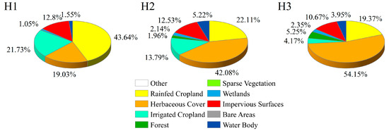
Figure 5.
Land cover for each cluster.
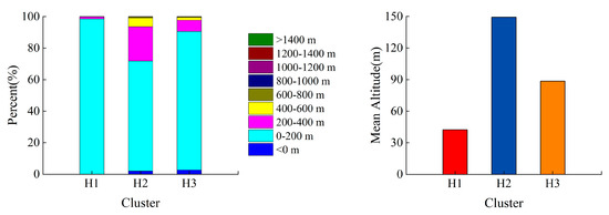
Figure 6.
DEM analysis results of each cluster.
The majority of the H1 cluster includes the plain southwest of Mountain Tai and Yimeng Mountains; however, a few points located south of Mountain Tai fall under H2. The total area constitutes 40.50% of Shandong Province, and the majority of the landscape is lowland plains, rising to a height of less than 200 m. H1’s ET0mean and ET0max are the highest among the three clusters, with ET0 reaching 2.4–3.0 mm/day in 165.73 months. The low representative point P119 is close to the Bohai Sea, while the high representative point P168 is near Shandong Province’s center and extends toward H2. The amount of cropland in H1 is comparatively considerable, comprising 21.73% irrigated and 43.64% rainfed cropland.
H2 is mostly situated in Mountain Tai and Yimeng Mountains, as well as the plain to the east and south of Mountain Tai and Yimeng Mountains; a few points are included in H1, and certain points of H1 and H3 are also included in H2. This cluster extends north to the plain near the Bohai Sea, with the highest mean altitude. The ET0mean and ET0max of H2 are lower than those of H1, but greater than those of H3; in particular, ET0 reached 2.4–3.0 mm/day in only 78.16 months, significantly less than H1. H1 contains the high representative point P47, while the low representative point P79 is situated south of the Yimeng Mountains. H2 comprises 22.11% rainfed and 13.79% irrigated cropland.
H3 mostly encompasses coastal areas in the east and southeast and accounts for 25.26% of Shandong Province, with a few locations overlapping with H2. The terrain is mostly hilly and mountainous. Among the three clusters, H3 has the minimum values of ET0mean, ET0max, ET0min, and ET0std, with ET0 reaching 2.4–3.0 mm/day in only 3.85 months, which is significantly less than H1 and H2. However, ET0 reached 0–0.6 mm/day in 442.63 months, which is the highest value. The high representative point P208 is close to the Bohai Sea and Laizhou Bay, and the low representative point P238 is to the east. The small agricultural area in H3 comprises 19.37% rainfed and 4.17% irrigated cropland.
3.2. Analysis of Clusters
Figure 7, Figure 8 and Figure 9 show the ET0 trends in H1, H2, and H3, respectively. Figure 10 shows the ET0 distribution map of Shandong Province in different periods. Figure 11 shows the box plot of residual distribution. Table 4 shows the evaluation criteria of different clusters, and Table 5 shows the Mann–Kendall results of the annual average ET0. Deep learning and DL were used to obtain the SAO-CNN-BiGRU-Attention, which are discussed below.
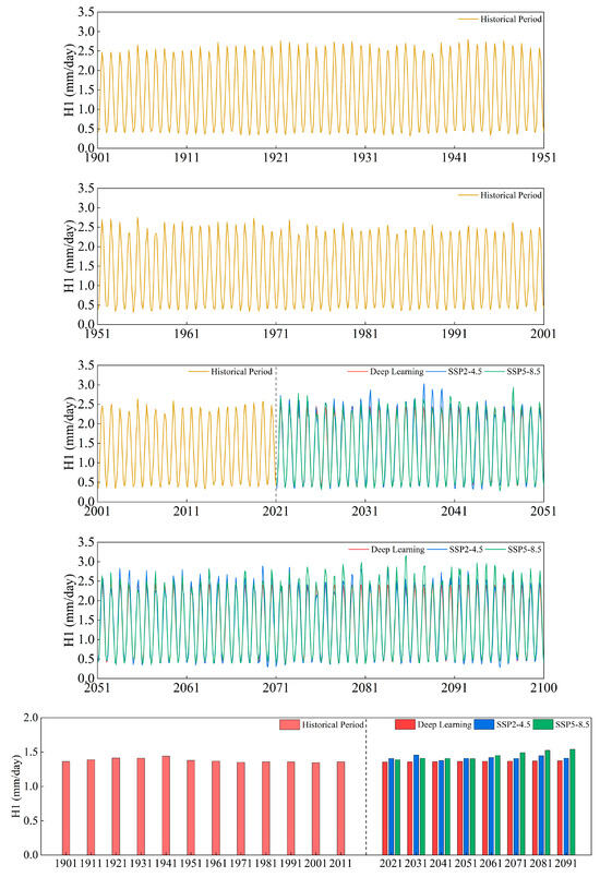
Figure 7.
The changing trend and ten-year average of ET0 in Cluster H1.
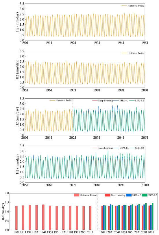
Figure 8.
The changing trend and ten-year average of ET0 in Cluster H2.
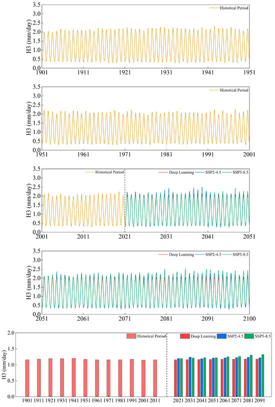
Figure 9.
The changing trend and ten-year average of ET0 in Cluster H3.
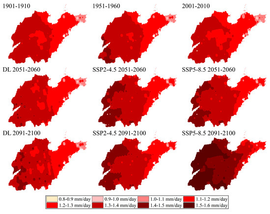
Figure 10.
ET0 distribution map of Shandong Province in different periods.
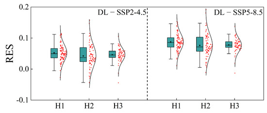
Figure 11.
Box plot of average residual; black dots indicate the average values.

Table 4.
Evaluation criteria of each cluster.

Table 5.
Mann–Kendall results (p and Slope) of annual average ET0 in each cluster.
The three clustering regions of H1, H2, and H3 showed monotonic declining trends from 1901 to 2020 (p < 0.001, Slope < 0). While the H1 and H2 SSP2-4.5 forecast trends were not significant (p > 0.05), the H1, H2, and H3 regions obtained using DL and SSP5-8.5 exhibited monotonically increasing trends (p < 0.001, Slope > 0). The ten-year average ET0 of the three clusters in 2021–2030 and 2031–2040 exhibited a tendency in the order of SSP2-4.5 > SSP5-8.5 > DL; from the period 2061–2070 until the conclusion of the projected period, the three cluster regions showed a trend of SSP5-8.5 > SSP2-4.5 > DL. For the ten-year average ET0, according to the DL results, H1, H2, and H3 will reach their peaks in 2091–2100, with 1.37 mm/day, 1.32 mm/day, and 1.18 mm/day, respectively. The SSP2-4.5 results indicate that H1, H2, and H3 will reach their peaks in 2031–2040, with 1.46 mm/day, 1.39 mm/day, and 1.24 mm/day, respectively. The SSP5-8.5 results indicate that during 2091–2100, H1, H2, and H3 will reach peaks of 1.54 mm/day, 1.47 mm/day, and 1.32 mm/day, respectively. The ten-year average ET0 of 2091–2100 demonstrated an increasing tendency when compared to that of 2021–2030. DL’s prediction for H1, H2, and H3 increased by 1.31%, 1.56%, and 1.80%, respectively, whereas the SSP2-4.5 forecasts for H1, H2, and H3 increased by 0.31%, 0.95%, and 1.57%, respectively, and the SSP5-8.5 forecasts for H1, H2, and H3 increased by 10.88%, 10.76%, and 10.69%, respectively.
In general, the DL prediction scores of the three cluster areas are closer to those of SSP2-4.5 and lower than those of SSP2-4.5 and SSP5-8.5; the R2 is higher, and the RMSE, MAE, and MAPE are lower when compared to SSP5-8.5. Additionally, Figure 10 shows that the box is lower and that the average values and medium number of residuals from the SSP2-4.5 prediction findings are lower. The DL prediction results contain some points and time periods greater than SSP2-4.5 and SSP5-8.5 within the forecast period, and in a few spots, the average residuals are less than zero, as seen in Figure 11. The DL analysis indicates that ET0 trend continues to follow the pattern of H1 > H2 > H3, meaning that inland regions will continue to have higher ET0 values than coastal areas. H1 has the highest ET0, followed by H2 and H3. A similar trend is observed in the ten-year average ET0 pillar chart using SSP2-4.5 and SSP5-8.5, which is shown in Figure 10; darker colors indicate inland regions.
3.3. Analysis of Representative Points
The ten-year average change in ET0 values of the high and low representative points are displayed in Figure 12 and Figure 13, respectively, with their evaluation criteria displayed in Table 6 and Table 7, respectively. The Mann–Kendall test results for the annual average ET0 of the high and low representative points are displayed in Table 8 and Table 9, respectively.
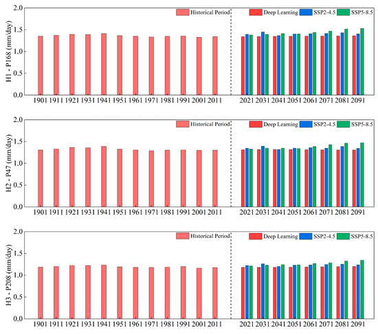
Figure 12.
Ten-year average ET0 of high representative points.
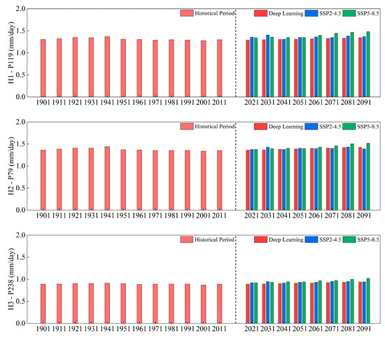
Figure 13.
Ten-year average ET0 of low representative points.

Table 6.
Evaluation criteria of high representative points.

Table 7.
Evaluation criteria of low representative points.

Table 8.
Mann–Kendall results (p and Slope) of annual average ET0 in high representative points.

Table 9.
Mann–Kendall results (p and Slope) of annual average ET0 in low representative points.
Considering the high representative points, H1, H2, and H3 steadily declined throughout the historical period (p < 0.001, Slope < 0). In H1 and H3, the future prediction values of DL and SSP5-8.5 exhibited a monotonically increasing trend (p < 0.001, Slope > 0). By contrast, in H2, SSP5-8.5 exhibited a monotonic upward trend (p < 0.001, Slope = 0.00224), whereas DL exhibited a monotonically decreasing trend (p < 0.001, Slope = −0.00046). The DL prediction results in the three clusters are closer to those of SSP2-4.5, with a greater R2 and lower RMSE and MAE than SSP5-8.5. All three cluster areas in the ten-year average ET0 of 2021–2030 and 2030–2040 exhibited a trend of SSP2-4.5 > SSP5-8.5 > DL; H1 and H3 revealed a pattern of SSP5-8.5 > SSP2-4.5 > DL for the 2041–2050 period, whereas H2 exhibited this trend for the 2061–2070 period. According to the DL predictions, H2 will peak in 2081–2090 at 1.31 mm/day, whereas H1 and H3 will peak in 2091–2100 at 1.36 mm/day and 1.20 mm/day, respectively. Based on SSP2-4.5 projections, in 2031–2040, the peaks of H1, H2, and H3 will be 1.48 mm/day, 1.39 mm/day, and 1.26 mm/day, respectively. According to the SSP5-8.5 results, H1, H2, and H3 are expected to peak in 2031–2040 at 1.53 mm/day, 1.47 mm/day, and 1.34 mm/day, respectively. In comparison to the results for 2021–2020, considering the ten-year average ET0 in 2091–2100, DL predicted an increase in H1 and H3 by 1.59% and 1.79%, respectively, and a decrease in H2 by 0.43%. SSP2-4.5 estimated an increase in H1 and H3 by 0.85% and 1.15%, respectively, and a decrease in H2 by 0.07%. SSP5-8.5 predicted an increase in H1, H2, and H3 by 10.82%, 11.09%, and 10.97%, respectively.
Regarding the low representative points, throughout the historical period, H1, H2, and H3 all experienced monotonic declines (p < 0.001, Slope < 0). The forecast trend of SSP2-4.5 was not significant (p > 0.05) in H1 and H2; however, all of the future predictions of DL and SSP5-8.5 exhibited an increasing trend (p < 0.001, Slope > 0) in the three clusters. The DL prediction results in the three clusters are closer to SSP2-4.5, with greater R2 and lower RMSE and MAE values than SSP5-8.5. H2 exhibited a trend of SSP5-8.5 > SSP2-4.5 > DL in 2021–2030, while H1 and H3 exhibited a SSP2-4.5 > SSP5-8.5 > DL pattern. For H1 and H3, the pattern was SSP5-8.5 > SSP2-4.5 > DL after 2061–2070. The predicted H1, H2, and H3 clusters peaked in 2091–2100 with respective velocities of 1.38 mm/day, 1.43 mm/day, and 0.95 mm/day. According to SSP2-4.5 results for 2031–2040, H1, H2, and H3 will reach their peaks at 1.38 mm/day, 1.43 mm/day, and 0.95 mm/day. According to SSP5-8.5, H1, H2, and H3 will peak at 1.48 mm/day, 1.52 mm/day, and 1.02 mm/day, respectively, in 2031–2040. Compared with the ten-year average ET0 of 2091–2100, for the years 2021–2020, the DL predictions in H1, H2, and H3 increased by 3.80%, 5.17%, and 5.58%, respectively; in SSP2-4.5, the predictive values increased by 0.85%, 1.18%, and 2.35%, respectively; in SSP5-8.5, the forecast increased by 10.53%, 10.18%, and 11.05%, respectively.
4. Discussion
From a spatial perspective, the eastern coastal region’s ET0 is lower than that of the western inland region, indicating a pattern of increasing westward; similarly, the southern region’s ET0 in Mountain Tai is lower than that of the northern region at the same longitude. From a clustering standpoint, the geographical and coastal characteristics are included in ET0; for example, low temperatures and ET0 may be found in mountainous and coastal regions [58]. The ET0 of land-based water bodies is likewise low, particularly for P54 in the southwest area of Shandong Province and P194 on the western edge of H3, suggesting that topography and land cover influence ET0. Previous research has demonstrated a comparatively high level of freshwater coverage [59]. The primary reason for this is that the HS equation alone takes into account the impact of temperature, while other meteorological elements may differ. The primary agricultural production regions are H1 and H2, which are located close to the inland region. Both rainfed and irrigated croplands are sizable and pose a significant need for agricultural water, particularly for winter wheat, which frequently needs three irrigation cycles with a 240 mm irrigation quota [60]. Although the amount of water used for agriculture will decrease, climate change will increase the amount of water needed for irrigation [61], and inland areas with high steam temperatures will require more intensive irrigation. These regions can adjust their planting model and employ different methods to save water for agricultural purposes.
A non-parametric Mann–Kendall test was used to determine the monotonic trend in sequence data, in which the number of continuous data points exhibiting an increasing or decreasing trend is determined to assess the trend’s intensity and direction [62]. The “evaporation paradox” reveals that evapotranspiration has been declining despite a notable rise in global temperatures [63]. Following the Mann–Kendall test, we determined the annual average ET0 for the historical period, and we found a monotonically declining trend, suggesting that Shandong Province is also experiencing a noteworthy “evaporation paradox” phenomenon, which may be associated with the effects of irrigation on agriculture and other activities [64]. Certain regions exhibit a monotonically declining trend during the forecast period, likely due to variations in surface resistance [65]. This demonstrates that different regions will require water supplies to varying degrees.
Deep learning methods are widely used to predict ET0 [21]. Compared with the original Penman–Monteith formula and Hargreaves–Samani formula, it does not need to include meteorological forcing data such as temperature and dew point, which are usually difficult to obtain [19]. However, the hyperparameters of deep learning models often need to rely on experience to obtain [66], and selecting inappropriate hyperparameters can increase the risk of overfitting and decreased accuracy [31]. In this research, the snow ablation optimizer algorithm was used to obtain the hyperparameters of the model’s learning rate and L2 regularization parameters, effectively improving the prediction capabilities of deep learning models for time series. The SAO-CNN-BiGRU-Attention deep learning model’s prediction accuracy was considerably greater than that of linear regression and other models. This is because, in Shandong Province, monthly changes were characterized by single-peak curves, with significantly higher values in summer than in winter [59]. The linear regression is not suitable for predicting future ET0.
While the SAO-CNN-BiGRU-Attention prediction findings in this article are generally lower than those of SSP2-4.5 and SSP5-8.5 and are more in line with SSP2-4.5, some of the points exhibit greater values than those of the two future scenarios, indicating that the predictions made using the SAO-CNN-BiGRU-Attention model are accurate. According to the Mann–Kendall test, ET0 will rise in the future, but each point’s peak value will have a distinct height and duration. The inland ET0 was still greater than the coastal ET0 in the forecast period, indicating a growing tendency from east to west. The SSP2-4.5 and SSP5-8.5 findings revealed a similar pattern. The annual fluctuations in ET0 exhibited single-peak characteristics throughout the historical and anticipated period [59], with winter presenting comparatively low values and summer exhibiting the highest, which are attributed to temperature characteristics. Furthermore, in future research, many GCMs, including BCC-CSM2-MR [67] and ACCESS-CM2 [68], may be considered, thus yielding more intriguing outcomes using different modes.
5. Conclusions
After hierarchical clustering, Shandong Province was found to encompass three homogeneous regions. The inland region had a greater ET0 than the coastal region since they are the primary agricultural production areas. Historically, the average yearly ET0 for the three regions decreased monotonically. The SAO-CNN-BiGRU-Attention and SSP5-8.5 domains showed a monotonic increasing trend in the three clusters, while the outcomes of a few points of the SAO-CNN-BiGRU-Attention predictions showed a monotonic decreasing trend.
According to the SAO-CNN-BiGRU-Attention results, during 2091–2100, H1, H2, and H3 will reach their peaks of 1.37 mm/day, 1.32 mm/day, and 1.18 mm/day, respectively; the SSP2-4.5 results show that H1, H2, and H3 will peak in 2031–2040, with 1.46 mm/day, 1.39 mm/day, and 1.24 mm/day, respectively; and the SSP5-8.5 results show that H1, H2, and H3 will reach their peaks in 2091–2100, with 1.54 mm/day, 1.47 mm/day, and 1.32 mm/day, respectively.
The SAO-CNN-BiGRU-Attention prediction outcomes were closer to those of SSP2-4.5. In comparison to 2021–2030, considering the ten-year average ET0 of 2091–2100 for H1, H2, and H3, the SAO-CNN-BiGRU-Attention forecasts increased by 1.31, 1.56%, and 1.80%, respectively; the SSP2-4.5 forecasts increased by 0.31%, 0.95%, and 1.57%, respectively; and the SSP5-8.5 forecasts increased by 10.88%, 10.76%, and 10.69%, respectively.
The SAO-CNN-BiGRU-Attention deep learning model’s prediction values were similar to those of SSP2-4.5 (R2 > 0.96), making it a promising method for future ET0 prediction.
Supplementary Materials
The following supporting information can be downloaded at: https://www.mdpi.com/article/10.3390/agriculture14091556/s1, Table S1: Experience-based hyperparameters; Table S2: R2 of the potential models. Reference [19] is cited in Supplementary Materials.
Author Contributions
Conceptualization, G.P.; methodology, Y.W.; software, X.F.; formal analysis, Y.W.; resources, Z.X.; writing—original draft preparation, Y.W.; writing—review and editing, G.P., T.W., X.C., X.W. and Z.X.; funding acquisition, G.P. and W.P. All authors have read and agreed to the published version of the manuscript.
Funding
This study was supported by the National Key Research and Development Program of China (2017YFD0800601), the National Natural Science Foundation of China (42307803), and the Natural Science Foundation of Shandong Province (ZR2020ME255).
Data Availability Statement
The original contributions presented in this study are included in the article/Supplementary Materials. Further inquiries can be directed to the corresponding author.
Acknowledgments
The datasets were provided by the National Tibetan Plateau/Third Pole Environment Data Center (http://data.tpdc.ac.cn, accessed on 10 April 2024).
Conflicts of Interest
The authors declare no conflicts of interest.
References
- Di Nunno, F.; Granata, F. Future trends of reference evapotranspiration in Sicily based on CORDEX data and Machine Learning algorithms. Agric. Water Manag. 2023, 280, 108232. [Google Scholar] [CrossRef]
- Bellido-Jiménez, J.A.; Estévez, J.; García-Marín, A.P. A regional machine learning method to outperform temperature-based reference evapotranspiration estimations in Southern Spain. Agric. Water Manag. 2022, 274, 107955. [Google Scholar] [CrossRef]
- Kim, S.; Hwang, S.; Song, J.-H.; Lee, H.; Kang, M.-S. Impact of irrigation reservoirs on budget of the watershed-scale water cycle under climate change. Agric. Water Manag. 2023, 283, 108327. [Google Scholar] [CrossRef]
- Li, X.; Xu, X.; Tian, W.; Tian, J.; He, C. Contribution of climate change and vegetation restoration to interannual variability of evapotranspiration in the agro-pastoral ecotone in northern China. Ecol. Indic. 2023, 154, 110485. [Google Scholar] [CrossRef]
- Goyal, R.K.; Gaur, M.K. The Implications of Climate Change on Water Resources of Rajasthan. In Hydro-Meteorological Extremes and Disasters; Goyal, M.K., Gupta, A.K., Gupta, A., Eds.; Springer Nature: Singapore, 2022; pp. 265–278. [Google Scholar]
- Huntington, T.G. Evidence for intensification of the global water cycle: Review and synthesis. J. Hydrol. 2005, 319, 83–95. [Google Scholar] [CrossRef]
- Ndiaye, P.M.; Bodian, A.; Diop, L.; Deme, A.; Dezetter, A.; Djaman, K.; Ogilvie, A. Trend and Sensitivity Analysis of Reference Evapotranspiration in the Senegal River Basin Using NASA Meteorological Data. Water 2020, 12, 1957. [Google Scholar] [CrossRef]
- Tan, X.; Jia, Y.; Yang, D.; Niu, C.; Hao, C. Turning points in the impact of earlier green-up on evapotranspiration and gross primary productivity in a semi-arid grassland watershed. J. Hydrol. 2023, 616, 128755. [Google Scholar] [CrossRef]
- Iqbal, M.; Wen, J.; Masood, M.; Masood, M.U.; Adnan, M. Impacts of Climate and Land-Use Changes on Hydrological Processes of the Source Region of Yellow River, China. Sustainability 2022, 14, 14908. [Google Scholar] [CrossRef]
- Lu, T.; Han, Y.; Dong, L.; Zhang, Y.; Zhu, X.; Xu, D. Evapotranspiration responses to CO2 and its driving mechanisms in four ecosystems based on CMIP6 simulations: Forest, shrub, farm and grass. Environ. Res. 2023, 223, 115417. [Google Scholar] [CrossRef]
- Rawat, K.S.; Bala, A.; Singh, S.K.; Pal, R.K. Quantification of wheat crop evapotranspiration and mapping: A case study from Bhiwani District of Haryana, India. Agric. Water Manag. 2017, 187, 200–209. [Google Scholar] [CrossRef]
- Subedi, A.; Chávez, J.L.; Andales, A.A. ASCE-EWRI standardized Penman-Monteith evapotranspiration (ET) equation performance in southeastern Colorado. Agric. Water Manag. 2017, 179, 74–80. [Google Scholar] [CrossRef]
- Xing, L.; Feng, Y.; Cui, N.; Guo, L.; Du, T.; Wu, Z.; Zhang, Y.; Wen, S.; Gong, D.; Zhao, L. Estimating reference evapotranspiration using Penman-Monteith equation integrated with optimized solar radiation models. J. Hydrol. 2023, 620, 129407. [Google Scholar] [CrossRef]
- Feng, Y.; Jia, Y.; Cui, N.; Zhao, L.; Li, C.; Gong, D. Calibration of Hargreaves model for reference evapotranspiration estimation in Sichuan basin of southwest China. Agric. Water Manag. 2017, 181, 1–9. [Google Scholar] [CrossRef]
- Kim, H.-J.; Chandrasekara, S.; Kwon, H.-H.; Lima, C.; Kim, T.-W. A novel multi-scale parameter estimation approach to the Hargreaves-Samani equation for estimation of Penman-Monteith reference evapotranspiration. Agric. Water Manag. 2023, 275, 108038. [Google Scholar] [CrossRef]
- Lu, Y.; Sun, L.; Li, C.; He, J.; Guo, Z.; Duan, L.; Zhang, J.; Łupikasza, E.; Malik, I.; Wistuba, M.; et al. Spatiotemporal Changes in and Driving Factors of Potential Evapotranspiration in a Hyper-Arid Locale in the Hami Region, China. Atmosphere 2024, 15, 136. [Google Scholar] [CrossRef]
- Ruperto, O.G.; Flowers-Cano, R.S.; Guillermo, M.G. Sensitivity of the RDI and SPEI Drought Indices to Different Models for Estimating Evapotranspiration Potential in Semiarid Regions. Water Resour. Manag. 2022, 36, 2471–2492. [Google Scholar] [CrossRef]
- Zhang, B.; Pan, Y.; Li, X. Revision Coefficient of Hargreaves Model and Its Values in Different Climatic Regions of China. Geogr. Geo-Inf. Sci. 2012, 28, 51–54. [Google Scholar]
- Jiang, Z.; Yang, S.; Dong, S.; Pang, Q.; Smith, P.; Abdalla, M.; Zhang, J.; Wang, G.; Xu, Y. Simulating soil salinity dynamics, cotton yield and evapotranspiration under drip irrigation by ensemble machine learning. Front. Plant Sci. 2023, 14, 1143462. [Google Scholar] [CrossRef]
- Hu, Y.; Liu, C.; Wollheim, W.M. Prediction of riverine daily minimum dissolved oxygen concentrations using hybrid deep learning and routine hydrometeorological data. Sci. Total Environ. 2024, 918, 170383. [Google Scholar] [CrossRef]
- Roy, D.K.; Sarkar, T.K.; Kamar, S.S.A.; Goswami, T.; Muktadir, M.A.; Al-Ghobari, H.M.; Alataway, A.; Dewidar, A.Z.; El-Shafei, A.A.; Mattar, M.A. Daily Prediction and Multi-Step Forward Forecasting of Reference Evapotranspiration Using LSTM and Bi-LSTM Models. Agronomy 2022, 12, 594. [Google Scholar] [CrossRef]
- Afzaal, H.; Farooque, A.A.; Abbas, F.; Acharya, B.; Esau, T. Computation of Evapotranspiration with Artificial Intelligence for Precision Water Resource Management. Appl. Sci. 2020, 10, 1621. [Google Scholar] [CrossRef]
- Saggi, M.K.; Jain, S. Reference evapotranspiration estimation and modeling of the Punjab Northern India using deep learning. Comput. Electron. Agric. 2019, 156, 387–398. [Google Scholar] [CrossRef]
- Wang, S.; Yu, X.; Li, Y.; Wang, S.; Meng, C. Application of a hybrid deep learning approach with attention mechanism for evapotranspiration prediction: A case study from the Mount Tai region, China. Earth Sci. Inform. 2023, 16, 3469–3487. [Google Scholar] [CrossRef]
- Wang, D.; Liu, J.; Huang, Y.; Shi, B.; Jin, M. Photovoltaic Power Prediction Method Combinating Solar Radiation Calculation and CNN-LSTM. Acta Energiae Solaris Sin. 2024, 45, 443–450. [Google Scholar] [CrossRef]
- Ferreira, L.B.; da Cunha, F.F. Multi-step ahead forecasting of daily reference evapotranspiration using deep learning. Comput. Electron. Agric. 2020, 178, 105728. [Google Scholar] [CrossRef]
- Chen, J.; Zhang, J.; Chen, H.; Zhao, Y.; Wang, H. A TDV attention-based BiGRU network for AIS-based vessel trajectory prediction. iScience 2023, 26, 106383. [Google Scholar] [CrossRef]
- Jamei, M.; Ali, M.; Bateni, S.M.; Jun, C.; Karbasi, M.; Malik, A.; Jamei, M.; Yaseen, Z.M. Short-term drought Index forecasting for hot and semi-humid climate Regions: A novel empirical Fourier decomposition-based ensemble Deep-Random vector functional link strategy. Comput. Electron. Agric. 2024, 217, 108609. [Google Scholar] [CrossRef]
- Song, Y.; Yang, S.; Zheng, L.; Ning, J. Semantic Segmentation Algorithm Based Multi-headed Self-attention for Tea Picking Points. Trans. Chin. Soc. Agric. Mach. 2023, 54, 297–305. [Google Scholar] [CrossRef]
- Dongxiao, N.; Min, Y.; Lijie, S.; Tian, G.; Keke, W. Short-term multi-energy load forecasting for integrated energy systems based on CNN-BiGRU optimized by attention mechanism. Appl. Energy 2022, 313, 118801. [Google Scholar]
- Bischl, B.; Binder, M.; Lang, M.; Pielok, T.; Richter, J.; Coors, S.; Thomas, J.; Ullmann, T.; Becker, M.; Boulesteix, A.L.; et al. Hyperparameter optimization: Foundations, algorithms, best practices, and open challenges. WIREs Data Min. Knowl. Discov. 2023, 13, e1484. [Google Scholar] [CrossRef]
- Deng, L.; Liu, S. Snow ablation optimizer: A novel metaheuristic technique for numerical optimization and engineering design. Expert Syst. Appl. 2023, 225, 120069. [Google Scholar] [CrossRef]
- Chen, H.; Ren, A.; Hu, Z.; Jia, C.; Wang, J. Effects of irrigation and fertilization on soil salt migration, yield, and water use efficiency of winter wheat in the Yellow River Delta. Crop Sci. 2022, 62, 1584–1602. [Google Scholar] [CrossRef]
- Zhang, F.; Liu, Z.; Zhangzhong, L.; Yu, J.; Shi, K.; Yao, L. Spatiotemporal Distribution Characteristics of Reference Evapotranspiration in Shandong Province from 1980 to 2019. Water 2020, 12, 3495. [Google Scholar] [CrossRef]
- Liu, X.; Li, X.; Gao, L.; Zhang, J.; Qin, D.; Wang, K.; Li, Z. Early-season and refined mapping of winter wheat based on phenology algorithms—A case of Shandong, China. Front. Plant Sci. 2023, 14, 1016890. [Google Scholar] [CrossRef]
- Li, Q.; Zhang, J.; Zhang, J.; Gao, H.; Chen, W.; Huang, J.; Guo, Y.; Yue, S.; Li, G. Spatial and temporal distribution characteristics and prediction analysis of nitrogen and phosphorus surface source pollution in Shandong Province under the climate and land use changes. Front. Ecol. Evol. 2023, 11, 1231394. [Google Scholar] [CrossRef]
- Zhang, P.; Ma, W.; Hou, L.; Liu, F.; Zhang, Q. Study on the Spatial and Temporal Distribution of Irrigation Water Requirements for Major Crops in Shandong Province. Water 2022, 14, 1051. [Google Scholar] [CrossRef]
- Gao, X.; Du, Z.; Yang, Q.; Zhang, J.; Li, Y.; Wang, X.; Gu, F.; Hao, W.; Yang, Z.; Liu, D.; et al. Energy partitioning and evapotranspiration in a black locust plantation on the Yellow River Delta, China. J. For. Res. 2021, 33, 1–14. [Google Scholar] [CrossRef]
- Dong, J.; Guo, M.; Wang, X.; Yang, X.; Zhang, Y.-H.; Zhang, P.-D. Dramatic loss of seagrass Zostera marina L. suitable habitat under projected climate change in coastal areas of the Bohai Sea and Shandong peninsula, China. J. Exp. Mar. Biol. Ecol. 2023, 565, 151915. [Google Scholar] [CrossRef]
- Zhao, Y.; Wang, X.; Guo, Y.; Hou, X.; Dong, L. Winter Wheat Phenology Variation and Its Response to Climate Change in Shandong Province, China. Remote Sens. 2022, 14, 4482. [Google Scholar] [CrossRef]
- Yu, M.; Xu, S.; Zhou, F.; Xu, H. A Study on the Relationship between Urban Spatial Structure Evolution and Ecological Efficiency in Shandong Province. Appl. Sci. 2024, 14, 818. [Google Scholar] [CrossRef]
- Liu, L.; Zhang, X.; Chen, X.; Gao, Y.; Mi, J. GLC_FCS30-2020: Global Land Cover with Fine Classification System at 30 m in 2020. Zenodo 2020. [Google Scholar] [CrossRef]
- Peng, S. 1-km monthly maximum temperature dataset for China (1901–2022). Earth Syst. Sci. Data 2020, 11, 1931–1946. Available online: https://data.tpdc.ac.cn/zh-hans/data/35ffff9f-8e1b-4296-801f-d8231e4f8dc3 (accessed on 29 July 2024).
- Peng, S. 1-km monthly minimum temperature dataset for China (1901–2022). Earth Syst. Sci Data 2020, 11, 1931–1946. Available online: https://data.tpdc.ac.cn/zh-hans/data/5b644091-5fbf-4cd8-9324-6a543c9c369f (accessed on 29 July 2024).
- Ding, Y.; Peng, S. Spatiotemporal Trends and Attribution of Drought across China from 1901–2100. Sustainability 2020, 12, 477. [Google Scholar] [CrossRef]
- Peng, S.; Ding, Y.; Liu, W.; Li, Z. 1 km monthly temperature and precipitation dataset for China from 1901 to 2017. Earth Syst. Sci. Data 2019, 11, 1931–1946. [Google Scholar] [CrossRef]
- Peng, S.; Ding, Y.; Wen, Z.; Chen, Y.; Cao, Y.; Ren, J. Spatiotemporal change and trend analysis of potential evapotranspiration over the Loess Plateau of China during 2011–2100. Agric. For. Meteorol. 2017, 233, 183–194. [Google Scholar] [CrossRef]
- Peng, S.; Gang, C.; Cao, Y.; Chen, Y. Assessment of climate change trends over the Loess Plateau in China from 1901 to 2100. Int. J. Climatol. 2017, 38, 2250–2264. [Google Scholar] [CrossRef]
- Sharma, S.; Hamal, K.; Khadka, N.; Ali, M.; Subedi, M.; Hussain, G.; Ehsan, M.A.; Saeed, S.; Dawadi, B. Projected Drought Conditions over Southern Slope of the Central Himalaya Using CMIP6 Models. Earth Syst. Environ. 2021, 5, 849–859. [Google Scholar] [CrossRef]
- Deng, Y.; Hou, P.; Jiang, W.; Peng, K.; Li, Z.; Deng, Y. Automatic Extraction of River Source Region Boundary based on Multi-Characteristic Indexes and Hierarchical Cluster Analysis. J. Geo-Inf. Sci. 2022, 24, 469–482. [Google Scholar] [CrossRef]
- Ros, F.; Riad, R.; Guillaume, S. PDBI: A partitioning Davies-Bouldin index for clustering evaluation. Neurocomputing 2023, 528, 178–199. [Google Scholar] [CrossRef]
- Meng, N.; Wang, L.; Qi, W.; Dai, X.; Li, Z.; Yang, Y.; Li, R.; Ma, J.; Zheng, H. A high-resolution gridded grazing dataset of grassland ecosystem on the Qinghai–Tibet Plateau in 1982–2015. Sci. Data 2023, 10, 68. [Google Scholar] [CrossRef]
- Wu, M.; Zhang, S.; Zhang, F.; Sun, R.; Tang, J.; Hu, S. Anomaly Detection Method for Lithium-Ion Battery Cells Based on Time Series Decomposition and Improved Manhattan Distance Algorithm. ACS Omega 2023, 9, 2409–2421. [Google Scholar] [CrossRef]
- Chen, X.; Cai, S.; Yu, L.; Li, X.; Fan, B.; Du, M.; Liu, T.; Bao, G. A Novel CNN-BiLSTM ensemble model with attention mechanism for sit-to-stand phase identification using wearable inertial sensors. IEEE Trans. Neural Syst. Rehabil. Eng. A Publ. IEEE Eng. Med. Biol. Soc. 2024, 32, 1068–1077. [Google Scholar] [CrossRef]
- Qian, Q.; Yu, J.; Zhan, H.; Wang, R.; Hu, J. Dimension prediction method of injection molded parts based on multi-feature fusion of DL-BiGRU. J. Zhejiang Univ. (Eng. Sci.) 2024, 58, 646–654. [Google Scholar] [CrossRef]
- Wang, J.; Xuan, K.; Xiong, H.; Wang, F.; Li, J. Beauty Pageant of Koi Method Based on Improved ResNeXt50 Residual Network. Trans. Chin. Soc. Agric. Mach. 2023, 54, 330–337. [Google Scholar] [CrossRef]
- Li, Z. An enhanced dual IDW method for high-quality geospatial interpolation. Sci. Rep. 2021, 11, 9903. [Google Scholar] [CrossRef]
- Gu, R.; Zhang, D.; Liao, A.; Shen, H.; Zhao, X.; Pan, J. On the Attribution of Changing Reference Evapotranspiration in a Coastal Area of China. Atmosphere 2018, 9, 9. [Google Scholar] [CrossRef]
- Li, H.; Chen, Z.; Jiang, Z.; Sun, L.; Liu, K.; Liu, B. Temporal-spatial variation of evapotranspiration in the Yellow River Delta based on an integrated remote sensing model. J. Appl. Remote Sens. 2015, 9, 096047. [Google Scholar] [CrossRef]
- Wang, T.; Xu, Z.; Pang, G. Effects of Irrigating with Brackish Water on Soil Moisture, Soil Salinity, and the Agronomic Response of Winter Wheat in the Yellow River Delta. Sustainability 2019, 11, 5801. [Google Scholar] [CrossRef]
- Sun, S.; Zhou, T.; Wu, P.; Wang, Y.; Zhao, X.; Yin, Y. Impacts of future climate and agricultural land-use changes on regional agricultural water use in a large irrigation district of northwest China. Land Degrad. Dev. 2019, 30, 1158–1171. [Google Scholar] [CrossRef]
- Mishra, S.; Chauhan, M.; Sundaramurthy, S. Assessment of Groundwater Trends in Bhopal, Madhya Pradesh: A Statistical Approach. Sustainability 2023, 15, 11971. [Google Scholar] [CrossRef]
- Cong, Z.; Ni, G.; Yang, D.; Lei, Z. Evaporation paradox in China. Adv. Water Sci. 2008, 19, 147–152. [Google Scholar] [CrossRef]
- Han, S.; Wang, S.; Yang, D. Agricultural influences on evaporation paradox in China. Trans. Chin. Soc. Agric. Eng. 2010, 26, 1–8. [Google Scholar]
- Gui, Y.; Wang, Q.; Zhao, Y.; Dong, Y.; Li, H.; Jiang, S.; He, X.; Liu, K. Attribution analyses of reference evapotranspiration changes in China incorporating surface resistance change response to elevated CO2. J. Hydrol. 2021, 599, 126387. [Google Scholar] [CrossRef]
- Li, W.; Yin, X.; Ye, M.; Zhu, P.; Li, J.L.; Yang, Y. Efficient hyperparameter optimization with Probability-based Resource Allocating on deep neural networks. Neurocomputing 2024, 599, 127907. [Google Scholar] [CrossRef]
- Sun, M.; Chou, J.; Xu, Y.; Yang, F.; Li, J. Study on the thresholds of grain production risk from climate change in China’s main grain-producing areas. Phys. Chem. Earth 2019, 116, 102837. [Google Scholar] [CrossRef]
- Chylek, P.; Folland, C.K.; Klett, J.D.; Wang, M.; Lesins, G.; Dubey, M.K. Why Does the Ensemble Mean of CMIP6 Models Simulate Arctic Temperature More Accurately Than Global Temperature? Atmosphere 2024, 15, 567. [Google Scholar] [CrossRef]
Disclaimer/Publisher’s Note: The statements, opinions and data contained in all publications are solely those of the individual author(s) and contributor(s) and not of MDPI and/or the editor(s). MDPI and/or the editor(s) disclaim responsibility for any injury to people or property resulting from any ideas, methods, instructions or products referred to in the content. |
© 2024 by the authors. Licensee MDPI, Basel, Switzerland. This article is an open access article distributed under the terms and conditions of the Creative Commons Attribution (CC BY) license (https://creativecommons.org/licenses/by/4.0/).