Research on a Variable Universe Control Method and the Performance of Large Sprayer Active Suspension Based on an Artificial Fish Swarm Algorithm–Back Propagation Fuzzy Neural Network

Abstract

In view of the typical requirements of large high-clearance sprayers, such as those operating in poor road conditions for farmland plant protection and at high operation speeds, reducing the vibration of sprayer suspension systems has become a research hotspot. In this study, the hydro-pneumatic suspension (HPS) of large high-clearance sprayers was taken as the object, and a variable universe T-S fuzzy controller with real vehicle vibration data as input was proposed to control suspension motion in real time. Different from traditional semi-active suspension, based on the characteristics of variable universe extension factors, a training method combining the artificial fish swarm algorithm and the back propagation algorithm was used to establish a fuzzy neural network controller with precise input to optimize the variable universe. Then, the time-domain and frequency-domain response characteristics of HPS were analyzed by simulating the special road conditions typical of farmland. Finally, the field performance of the sprayer equipped with the new controller was tested. The results show that the error rate of the AFSA-BP algorithm in training the FNN could be reduced to 3.9%, and compared with a passive suspension system, the T-S fuzzy controller improved the effects of spring mass acceleration, pitch angle acceleration, and roll angle acceleration by 18.3%, 23.3%, and 27.7%, respectively, verifying the effectiveness and engineering practicality of the active controller in this study.

1. Introduction

As the main spraying machine in the field plant protection process, large high-clearance sprayers play an indispensable role in agricultural production. With the developing trend of efficient and intelligent agricultural machinery production, large high-clearance sprayers are increasingly being widely used because of their strong environmental adaptability and high operating efficiency [1,2]. The core working conditions of large high-clearance sprayers, i.e., sensitivity to pesticide application and bumps experienced during road transportation to fields, lead to a contradiction between field driving safety and ride comfort, which cannot be solved by passive suspension based on tire damping or traditional semi-active suspension based on air spring damping. The problems caused by driving comfort and handling safety under high-speed road transportation seriously affect the working quality of large high-clearance sprayers. As an active suspension structure scheme for vibration reduction, HPS has become an important research topic in military and engineering vibration reduction fields due to its advantage of wide-range damping adjustment [3,4].

Active hydro-pneumatic suspension relies on a controller to adjust the opening of a solenoid valve in real time to perform oil charging and discharging of the suspension, and output the active control force for the body to cope with the road excitation [5,6,7]. Although there has been little research on active vibration reduction control in the field of sprayers, researchers in other vehicle domains have extensively examined suspension control with ride comfort as the research goal, in order to fully assess the system efficiency of HPS. Karnopp et al. assumed that a skyhook damper was installed between the inertial coordinate system and the vehicle body, and the vehicle body vibration was suppressed by the damping force generated by the skyhook damper [8]. On this basis, the researchers successively proposed skyhook control, triple skyhook control, hybrid skyhook–ground control, optimal control with reference to the skyhook, fuzzy skyhook control, and other algorithms, which improved the body vibration to a certain extent [9]. In addition, the application of modern control theory to improve vehicle dynamic performance has gradually become mainstream, and algorithms such as linear quadratic regulators, fuzzy control, and sliding mode control have been applied in a wide range of scenarios in the field of suspension vibration reduction. Matthias et al. transmitted information collected by a sensor to a model predictive controller to improve the active suspension performance of an autonomous vehicle [10]; Meng Jianjun et al. optimized a fuzzy PID controller based on the PSO algorithm, improving the smoothness of high-speed train operation [11]; Chen et al. proposed a sliding mode controller integrating SSOB and SMC, which adjusted the damping characteristics of a magnetorheological damper by controlling the adjustable current to improve the robustness of the damping system [12]; and inspired by the non-ideal state of an actuator, Pusadkar et al. designed a sliding mode controller based on a linear disturbance observer to improve the adverse effects of dead zones and lag of a hydraulic actuator [13]. The various control algorithms used in the above studies have provided effective control ideas for suspension system vibration reduction; however, most of them have only focused on the nonlinear effects inside a system during the vibration reduction process, and study suspension performance by simulating road roughness. However, for field working environments with high degrees of randomness, complex interactions between crops and soil, and large uncertainty of bumps, there is still no model that can accurately reflect field road excitation, and control methods for a single road shape cannot meet the working requirements of large sprayers.

Variable universe T-S fuzzy control can not only avoid uncertainty and approximate a controlled object with arbitrary precision by taking the actual signal as the input, but it can also control the steady-state error without adding fuzzy rules and fuzzy partitions, which has strong theoretical applicability in dealing with field environments [14,15]. However, the uncertainty of the variable universe expansion factor greatly reduces the control accuracy of the variable universe T-S fuzzy control algorithm and loses the original advantages of the algorithm. In view of the above problems, most researchers have used multi-objective optimization algorithms, mathematical operations, and other methods to describe the size of the expansion factor [16], but the description method is not ideal for domain control. Artificial intelligence algorithms have extensive applications in fields, such as in planting machinery and agricultural robots [17,18], for example, the promotion of neural network algorithms in obstacle avoidance and path planning for agricultural robots, and the application of machine vision algorithms in crop row monitoring, crop edge detection, and other areas. Fuzzy neural networks (FNNs), such as artificial intelligence algorithms, have the ability to handle nonlinear fuzzy systems, and also exhibit optimization functions of neural networks [19,20]. Cao et al. proposed a method to adjust the scaling factor of fuzzy controllers based on a fuzzy neural network, utilizing the beneficial FNN characteristics of using actual data records for training and online adaptive adjustment [21]. In view of the dependence of FNNs on the parameters to be determined, when defining these parameters, the back propagation (BP) algorithm is widely used in training the feedforward neural network, due to its advantages in solving complex internal mechanisms [22]. Similarly, the BP algorithm is extremely dependent on the selection of initial values and can easily fall into local optima, which makes the design of this kind of controller uncertain. The artificial fish swarm algorithm (AFSA) [23] has emerged as a model optimization algorithm due to its strong global search ability. However, its high complexity, late maturity, and weak local search ability stand in contrast to the premature and weak global search ability of the BP algorithm. Effectively integrating the advantages of the two algorithms is key to improving the accuracy of fuzzy control.

Based on this, considering the advantages of slow convergence speed and low dependence on the initial values of the AFSA, this paper innovatively introduces the AFSA in the optimization of an FNN as follows. (1) Actual road surface information in the field was collected and a Kalman filter vehicle body state observer was constructed; (2) taking the actual road information as the input, the variable universe T-S fuzzy control method based on the AFSA-BP algorithm to optimize the FNN cooperative controller was studied, and an active HPS controller based on the actual working environment was established to verify the advantages of introducing the AFSA into the controller; and (3) the effect of the controller was verified through a simulation of typical working conditions and a real vehicle test.

2. Materials and Methods

2.1. Establishment of Mathematical Model for the Suspension of Large High-Clearance Sprayer

2.1.1. Establishment of an HPS System Model

An HPS system comprises a hydraulic cylinder, an accumulator (1), a proportional valve (2), a two-position two-way proportional valve (3), and adjustable throttle valves (4 and 5). The suspension damping is adjusted by regulating the openings of the proportional valve and the throttle valves. When the sprayer is operating, the proportional valve (2) is opened, and the hydraulic cylinder and the accumulator are jointly controlled by the adjustable throttle valves (4 and 5), and a semi-active vibration reduction effect is achieved by altering the damping force.

In this study, an active suspension system was designed according to the vibration reduction requirements of various working conditions for the sprayer, as shown in Figure 1. The system comprises a proportional drop valve (6), a proportional lift valve (7), an overflow valve (8), and a differential pressure reducing valve (9). When large high-clearance sprayers operate in the field, the active suspension system is activated, and the proportional lift valve and the proportional drop valve adjust the flow of oil in real time according to the fluctuation of the road surface. This serves to mitigate vibrations, addressing the limitation of passive HPS systems that only adjust suspension damping characteristics through proportional valves and throttle valves, thus enabling active vibration reduction functionality.

Specifically, when significant road fluctuations are detected by the accelerometer, the active suspension system is activated, and the proportional lift valve (7) and proportional drop valve (6) are charged and discharge oil in real-time based on the road surface undulations, playing a role in mitigating vibrations. When it comes to dented pavement, the proportional lift valve (7) is opened. Under the action of the oil pump, hydraulic oil passes through the differential pressure reducing valve (9), proportional lift valve (7), and adjustable throttle valve (5), entering the rodless chamber of the hydraulic cylinder. This causes the hydraulic cylinder to extend, counteracting the impact of the sunken road surface on the entire vehicle. Conversely, when encountering a raised road surface, the proportional drop valve (6) is opened, and hydraulic oil flows from the hydraulic cylinder to the proportional drop valve (6), ultimately returning to the hydraulic tank.

During the calculation, the local pressure loss and pressure loss throughout the oil flow process are taken into account, Assuming that the displacement of the piston rod in the hydraulic cylinder is x_L, the output force of the HPS is decomposed into elastic force F_s and damping force F_c [24], which is defined by

$$\begin{array}{l}F=F_s+F_c\\ \hspace{1em}=m_{s}g{\left(\frac{p_{a0}{V}_{a0}}{p_{a0}{V}_{a0}-m_{s}g{x}_L}\right)}^r-\frac{75A_2}{\mathrm{Re}}\frac{L{\dot{x}}_L^2}{d_q}\mathrm{sign}({\dot{x}}_L)\\ \hspace{1em}-\frac{A_2}{2}\rho {\left[\frac{Q_2}{C_d(A_{m1}+A_{m2})}\right]}^2\mathrm{sign}({\dot{x}}_L)\\ \hspace{1em}+\rho A_2{\left(\frac{Q_1}{A_3}\right)}^2\left[{\xi }_1\left(0.5-0.5\mathrm{sign}\left({\dot{x}}_L\right)\right)-{\xi }_2\left(0.5+0.5\mathrm{sign}\left({\dot{x}}_L\right)\right)\right] \\ \hspace{1em} -\rho A_2{\left(\frac{Q_2}{A_3}\right)}^2•\left[{\xi }_3\left(0.5+0.5\mathrm{sign}\left({\dot{x}}_L\right)\right)-{\xi }_4\left(0.5-0.5\mathrm{sign}\left({\dot{x}}_L\right)\right)\right]\\ \hspace{1em}+\left(-\frac{1}{2}\rho {\left(\frac{Q_3}{C_d{A}_{1d}}\right)}^2\mathrm{sign}({\dot{x}}_L)-\frac{75}{\mathrm{Re}}\frac{L{\dot{x}}_L^2}{2d_q}\mathrm{sign}({\dot{x}}_L)\right)\left(A_1-A_2\right)\end{array}$$

(1)

where r is the gas polytropic index; m_s is the front wheel’s sprung mass, kg; p_a0 is the gas initial pressure, Pa; V_a0 is the gas initial volume, m³; A₁ is the rodless cavity’s effective area, m²; A₂ is the rod cavity’s effective working area, m²; A₃ is the pipeline cross-sectional area, m²; A_m1 is the proportional valve’s flow area, m²; A_m2 is the throttle valve’s flow area, m²; d_q is the pipeline inner diameter, m; L is the pipeline length, m; Q₁ is the oil flow rate in the rodless chamber, m³/s; Q₂ is the oil flow rate in the rod chamber, m³/s; Q₃ is the oil flow rate towards the accumulator, m³/s; C_d is the flow coefficient; A_1d is the cross-sectional area of the accumulator interface, m²; Re is the Reynolds number, 2000; ξ₁, ξ₂, ξ₃, and ξ₄ are the pressure loss coefficient from the oil pipe to the rodless chamber, the pressure loss coefficient from the rodless chamber to the oil pipe, the pressure loss coefficient from the rodless chamber to the oil pipe, and the pressure loss coefficient from the oil pipe to the rod-shaped chamber. Q₁ and Q₂ are determined as the product of the effective working area and operating speed. Q₃ is the difference between Q₁ and Q₂. The known quantities in Equation (1) are listed in

Table 1. Parameters of hydro-pneumatic suspension system.

Parameter	Symbol	Reference Value
Hydraulic oil density/kg·m−3	ρ	900
Front wheel spring mass/kg	ms	2100
Gas polytropic index	r	1.4
Effective working area of rodless chamber/m2	A1	0.6358
Effective working area of rod chamber/m2	A2	0.4768
Accumulator initial pressure/Pa	pa0	5,000,000
Accumulator initial volume/m3	Va0	0.0014
Flow Coefficient	Cd	0.68
Pipe diameter/m	dq	0.012
Oil pipe length/m	L	1
Accumulator interface cross-sectional area/m2	A1d	0.05

.

2.1.2. Establishment of a Complete Vehicle Model with the HPS

In actual operation, sprayers are required to assume additional transportation and transfer functions, necessitating a suspension system with superior handling performance. To address this, the vertical shaft-independent suspension was adopted in this study, and the hydraulic cylinder was vertically arranged between the motor and the vehicle body. Through the independent control of the four wheels, the suspension vibration reduction and strength assurance were realized, as shown in Figure 2. Unlike traditional non-independent suspensions, where the left and right wheels may interfere with each other, the wheels in this system were designed not to interfere, thereby enhancing ground contact performance and effectively improving the maneuverability and smoothness of the sprayer during high-speed transportation.

When a sprayer operates in the field, it encounters vibration issues such as vertical jumps, pitch changes, and roll changes. To analyze the vibrational characteristics of the suspension in large high-clearance sprayers, a 7-DOF dynamic model of its HPS was developed. This model comprises the vehicle body and four single-wheel suspensions. Assuming the vehicle mass is m_ts; θ and φ signify the vehicle body’s roll and pitch angles in an inertial frame; k_tij and c_tij signify the stiffness and damping of four tires, respectively; k_sij and c_sij signify the stiffness and damping of the rear suspension, respectively; m_uij signifies the four wheels’ unsprung mass, respectively; f_i (i = 1~4) signify the four wheel active control forces, respectively. This model includes seven degrees of freedom, comprising the body’s roll angle, pitch angle, and vertical displacement, along with the vertical displacement of four sets of spring masses. The overall vehicle state in static equilibrium is taken as the initial position, and the dynamic equations of each system parameter can be obtained from the d’Alembert theorem [25]:

$$\left\{\begin{array}{l}{m}_{ts}{\ddot{z}}_b=F_{FL}+F_{FR}+F_{RL}+F_{RR}-m_{ts}g+{\displaystyle \sum _{i=1}^4{f}_i}\\ J_p\ddot{\phi }=(F_{RL}+F_{RR}+f_3+f_4)b-(F_{FL}+F_{FR}+f_1+f_2)a\\ J_r\ddot{\theta }=(F_{FL}-F_{FR}+f_1-f_2)\cdot l/2+(F_{RL}-F_{RR}+f_3-f_4)\cdot l/2\end{array}\right.$$

(2)

where J_p is the pitch angle acceleration, rad/s²; J_r is the roll angle acceleration, rad/s²; z_b is the displacement of the body’s center of mass, m; F_ij is the suspension output force of each wheel, N; a is the front axle length, m; b is the rear axle length, m; l is the track width, m.

Utilizing Equation (1), the differential equation for the unsprung motion of each set of suspensions [26] is:

$$\left\{\begin{array}{l}{m}_{uFL}{\dot{z}}_{uFL}=-F_{FL}-m_{uFL}g-k_{tFL}(z_{uFL}-q_{FL})-c_{tFL}({\dot{z}}_{uFL}-{\dot{q}}_{FL})\\ m_{uFR}{\dot{z}}_{uFR}=-F_{FR}-m_{uFR}g-k_{tFR}(z_{uFR}-q_{FR})-c_{tFR}({\dot{z}}_{uFR}-{\dot{q}}_{FR})\\ m_{uRL}{\dot{z}}_{uRL}=-F_{RL}-m_{uRL}g-k_{tRL}(z_{uRL}-q_{RL})-c_{tRL}({\dot{z}}_{uRL}-{\dot{q}}_{RL})\\ m_{uRR}{\dot{z}}_{uRR}=-F_{RR}-m_{uRR}g-k_{tRR}(z_{uRR}-q_{RR})-c_{tRR}({\dot{z}}_{uRR}-{\dot{q}}_{RR})\end{array}\right.$$

(3)

where m_uij is each wheel’s unsprung mass, N; z_uij is each wheel’s unsprung displacement, m; q_ij is each wheel’s road excitation displacement, m.

Given that all four-wheel suspensions employ hydro-pneumatic springs, the output force of each wheel suspension [27] can be expressed as:

$$\left\{\begin{array}{l}{F}_{FL}=p_{1FL}{A}_1-p_{2FL}{A}_2\\ F_{FR}=p_{1FR}{A}_1-p_{2FR}{A}_2\\ F_{RL}=p_{1RL}{A}_1-p_{2RL}{A}_2\\ F_{RR}=p_{1RR}{A}_1-p_{2RR}{A}_2\end{array}\right.$$

(4)

where p_1ij is the rodless chamber pressure, MPa; p_2ij is the suspension rod chamber pressure, MPa.

When the variation range of the roll and pitch angles of the sprayer is relatively small, it can be assumed that sinθ = θ and sinφ = φ. Under these conditions, the geometric relationship between the suspension and the body connection position [28] is as follows:

$$\left\{\begin{array}{l}{z}_{sFL}=z_b-a\phi +\frac{l}{2}\theta ,\hspace{1em}{\dot{z}}_{sFL}={\dot{z}}_b-a\dot{\phi }+\frac{l}{2}\dot{\theta }\\ z_{sFR}=z_b-a\phi -\frac{l}{2}\theta ,\hspace{1em}{\dot{z}}_{sFR}={\dot{z}}_b-a\dot{\phi }-\frac{l}{2}\dot{\theta }\\ z_{sRL}=z_b+b\phi +\frac{l}{2}\theta ,\hspace{1em}{\dot{z}}_{sRL}={\dot{z}}_b+b\dot{\phi }+\frac{l}{2}\dot{\theta }\\ z_{sFL}=z_b+b\phi -\frac{l}{2}\theta ,\hspace{1em}{\dot{z}}_{sFL}={\dot{z}}_b+b\dot{\phi }-\frac{l}{2}\dot{\theta }\end{array}\right.$$

(5)

In this study, a self-developed large sprayer is considered as the primary research object, with its parameters detailed in

Table 2. Parameters of large high-clearance sprayer.

Parameter	Symbol	Reference Value
Sprayer front axle length/m	a	2.3
Sprayer rear axle length/m	b	2.3
Track width/m	l	1.9
Accumulator volume/L	V	3.5
Overall weight/kg	mts	7600
Tire stiffness coefficient/N·m−1	ktij	700,000
Tire damping coefficient/Ns·m−1	ctij	2400

.

2.1.3. Road Excitation Input

Given the intricacies of road conditions in field transportation of large sprayers, it is necessary to collect accurate road information for the indoor simulation test of a controller to simulate the real-time vibration characteristics of the field transportation without active damping. Therefore, a three-axis acceleration sensor (Bewis sensing, Wuxi, China) is positioned at the center of mass of the entire sprayer, enabling real-time monitoring of the body’s three-axis motion state. The acceleration sensor signal is then transmitted instantaneously via the sprayer’s data acquisition system and stored on the personal computer. The transportation scenarios for sprayers are mostly farmland and cement roads, specifically Class C and D roads. We assume that the sprayer travels on the same type of road for a sufficiently long period, such as operating at a speed of 20 km/h on Class C and D roads, and utilize the acceleration sensor signals as a dataset for controller input, as shown in Figure 3.

2.1.4. Establishment of An Active Control Force Model

The active controller adjusts the opening of the valve port by controlling the voltage value input to the proportional solenoid valve, thereby adjusting the active control force in the hydraulic cylinder. To accurately establish the correlation between the active control force and the voltage value, and to further characterize the dynamic performance of the valve-controlled hydraulic cylinder, the following equation is derived by modifying the fundamental equation of the valve-controlled hydraulic cylinder, assuming negligible oil compressibility [29].

$$K_q\cdot x_v=C_{d1}\cdot w\sqrt{\frac{1}{\rho }\left(P_s-P_L\right)}\cdot x_v=A_p\cdot d{x}_p$$

(6)

where K_q is the flow gain; x_v is the spool displacement, m; C_d1 is the hydraulic cylinder’s total leakage coefficient; w is the valve port area gradient; P_s is the system oil supply pressure, MPa; P_L is the load pressure, MPa; A_p is the hydraulic cylinder’s effective working area, m²; x_p is the hydraulic cylinder’s displacement, m.

Based on the design characteristics of the solenoid valve, x_v is equivalent to the product of the conversion gain K and the control voltage u. By considering the load pressure P_L as the ratio between the active control force and the piston rod area, the relationship between the active output force f and the control voltage [29] can be expressed as follows:

$$f=\left[P_s\cdot A_2-\rho A_2\cdot {\left(\frac{A_p\cdot d{x}_p}{C_d\cdot w}\right)}^2\right]/K\cdot u$$

(7)

where ρ is the density of the hydraulic oil, kg/m³.

2.2. Design of a Variable Universe Fuzzy Neural Network Vibration Reduction Controller for Sprayers

To achieve active vibration reduction in a sprayer, it is essential to regulate the valve opening based on the real-time input conditions of suspension and road surface to modulate the oil charging and discharging. In this study, variable universe T-S fuzzy control is employed to develop an active suspension controller whose control strategy is model-independent. To mitigate errors, a dynamic universe approach is utilized to approximate the ideal output of the T-S fuzzy controller. Addressing the challenge of accurately describing the expansion factor in variable universe control, a fuzzy neural network (FNN) control strategy optimized through a hybrid optimization of the AFSA and BP algorithms is introduced to refine the expansion factor. The detailed process is shown in Figure 4. Specifically, by utilizing the distinct effects of the AFSA and BP algorithms during the optimization iteration, a balance between global optimization and local optimization is achieved. By sequentially training the unknown parameters of the FNN controller, a dynamic response relationship is established between the variable universe T-S fuzzy controller and the vehicle model, thus enabling the output of active control force.

2.2.1. State Observer

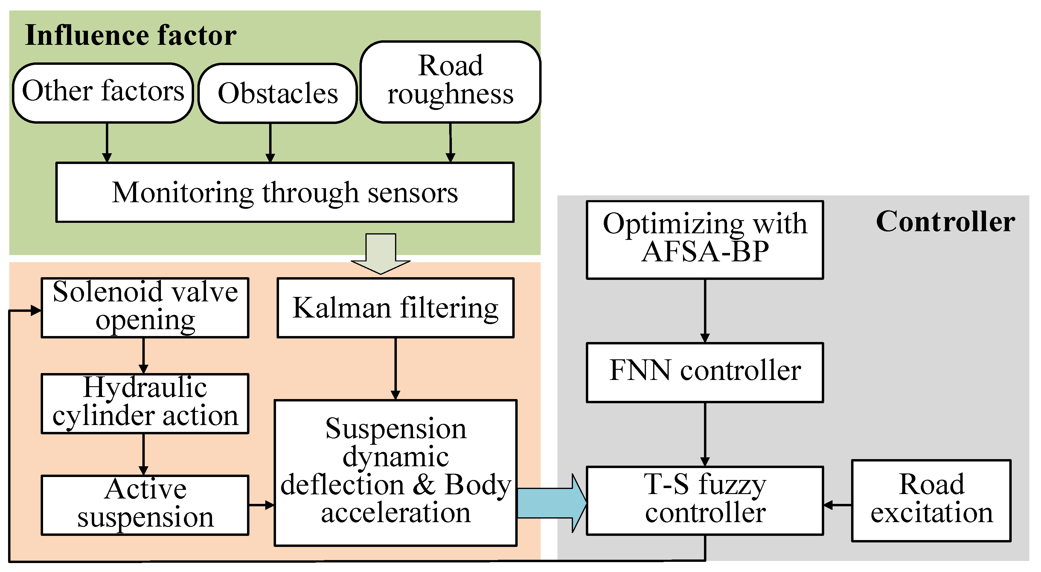
Due to spatial constraints and technological limitations under harsh working conditions, critical parameters such as sprung mass velocity during the operation of sprayers are often unattainable through sensor measurements. Moreover, the method of integrating and transforming signals received from acceleration sensors is prone to system drift and noise interference, resulting in significant errors in the converted data and subsequently affecting the accuracy of the observation state. To precisely monitor the suspension’s operating status and provide real-time running state input for active vibration reduction, a state observer based on Kalman filter is established based on the acceleration signal received by the body acceleration sensor. This approach enables the estimation and prediction of the suspension state.

Given the limitation of authenticating the state observer’s veracity through actual vehicle testing, it is imperative to establish a Simulink-based random road input model and integrate it into the suspension 1/4 dynamic model to validate the model’s effectiveness. The sprung mass velocity and unsprung mass velocity are used as control groups, and the estimated values of the Kalman filter are compared. The differential of the road input displacement [27] is shown as follows:

$${\dot{x}}_e\left(t\right)=-2\mathsf{\pi }{v}_t{n}_0{x}_e\left(t\right)+2\mathsf{\pi }\sqrt{G(n_0)v_t}w(t)$$

(8)

where v_t is the vehicle speed, m/s; n₀ is the k, taken as 0.011 m⁻¹; G(n₀) is the road surface roughness coefficient, m²/m⁻¹; w(t) is the mean value, taken as 0.

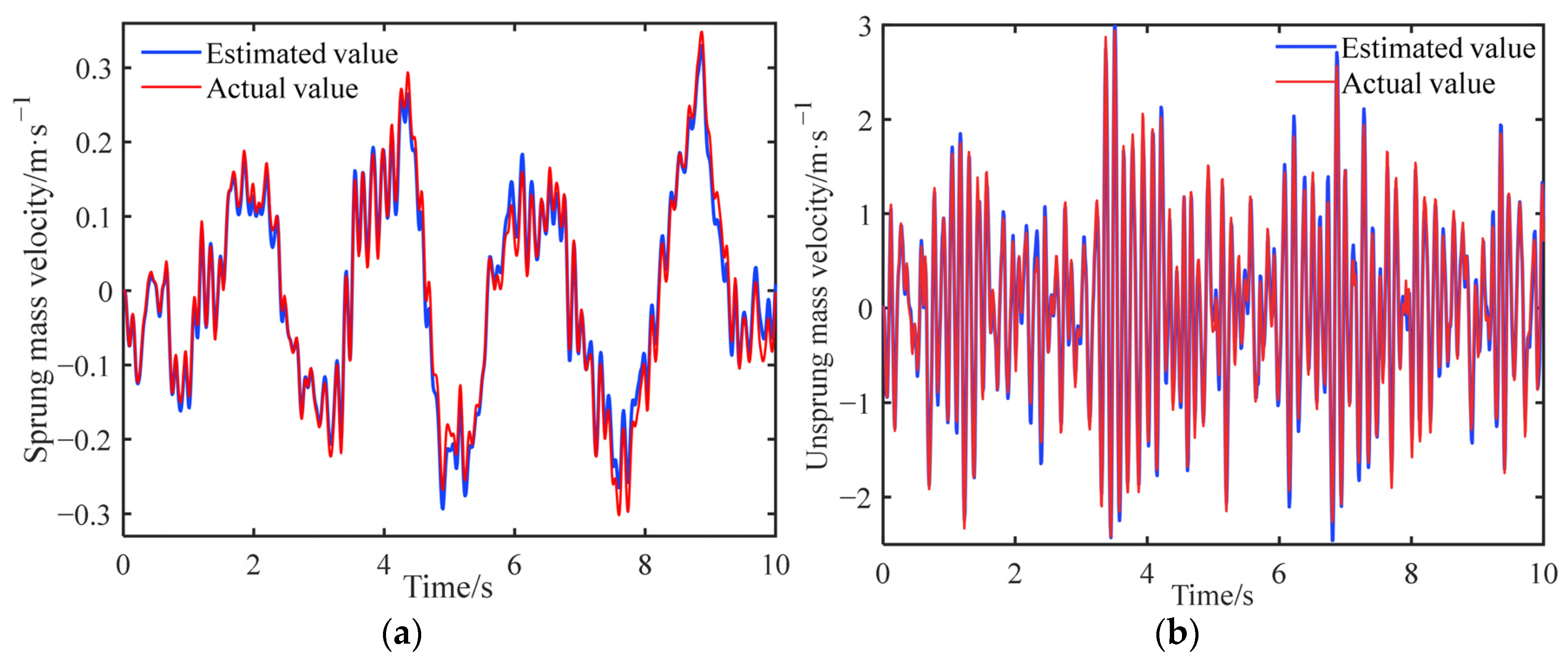
Utilizing the Class D road as a case study, the sprung mass velocity and unsprung mass velocity of the sprayer are estimated based on the acceleration sensor signals gathered at the sprung mass location, as detailed in Section 2.1.3. These estimates are then compared against the theoretical values derived from the road input model to ascertain the prediction outcomes of the state observer, as shown in Figure 5.

Based on the simulation curve depicted in Figure 5, it is evident that the suspension parameters derived through Kalman filtering exhibit a robust correlation with the actual state, manifesting a consistent fluctuation pattern and a substantial overlap between the respective curves. To further gauge the tracking proficiency of the observed values against the actual values, a tracking performance evaluation metric is introduced, as shown in the following equation [30].

$$E_r=\left[1-\frac{\sqrt{{\displaystyle \sum _{n=1}^N{\left(z-z’\right)}^2}}}{\sqrt{{\displaystyle \sum _{n=1}^N{z}^2}}}\right]\times 100\%$$

(9)

where z is the true value of the observed signal; z′ is the estimated value of the observed signal; N is the data number.

After substituting the data into the calculations, the curve fitting degrees of the sprung mass acceleration and the unsprung mass acceleration are 79.22% and 81.62%, respectively. For the hydro-pneumatic suspension exhibiting strong nonlinear characteristics, the Kalman filter can effectively observe the motion state of the suspension system, and the estimated value is within the reasonable error range, which proves the effectiveness of the Kalman filter observer, addressing the issue of the system state being unmeasurable, and providing the basis for parameter input for the subsequent design of an active vibration reduction controller.

2.2.2. Design of a Variable Universe T-S Fuzzy Controller

The unevenness of the road surface during the transportation of sprayers will greatly impact the body. As the core component of the sprayer’s vibration reduction mechanism, the HPS exhibits a strong nonlinear characteristic when excited by the road surface, thus posing high requirements on the design of active vibration reduction systems. Achieving a good vibration reduction effect using traditional linear control methods is challenging. To address these issues, this study introduces the T-S fuzzy controller, a nonlinear control method characterized by semi-linearization. The fuzzy field is adjusted using the variable universe method to improve control accuracy.

The complexity of fuzzy rules in complex systems can effectively enhance the accuracy of voltage control. However, as the complexity of these rules increases, so does the steady-state error of the T-S fuzzy controller. Furthermore, the traditional fixed universe control method poses a higher risk of system overshoot when the universe is set narrowly. To address this issue, the variable universe theory was introduced, precisely expanding or contracting the universe in accordance with the changes in system input and output, thereby achieving real-time high-precision control [14]. The range of dynamic adjustment for the universe is as follows:

$$\left\{\begin{array}{l}{X}_i(x_i)=\left[-{\alpha }_i(x_i)E_i {\alpha }_i(x_i)E_i\right]\\ Y(y)=\left[-\beta (y)C \beta (y)C\right]\end{array}\right.$$

(10)

where X_i(x_i) and Y(y) are the fuzzy domains of input and output variables, x_i (i = 1, 2, …, n); [−E, E], [−C, C] are the initial domains; α_i and β are the expansion factors for input and output.

The boundaries of the fuzzy universe are dynamically adjusted by altering the expansion factor. Given that the variable universe T-S fuzzy controller regulates the opening of the valve port via the control voltage output to the proportional solenoid valve, the initial universe is set to (−5, 5), and seven fuzzy subsets are employed: {NB (negative big), NM (negative middle), NS (negative small), ZO (zero), PS (positive small), PM (positive middle), and PB (positive big)}. The controller inputs comprise the sprung mass acceleration value captured by the acceleration sensor and the sprung mass velocity estimate derived from the Kalman filter. Based on these considerations, the T-S fuzzy controller is designed according to the following equation [31]:

$$\left\{\begin{array}{l}{g}_{ij}\left(X\right)=a_{ij0}+a_{ij1}{x}_1+a_{ij2}{x}_2+\cdot \cdot \cdot +a_{ijn}{x}_n\\ g_j\left(X\right)={\displaystyle \sum _{i=1}^v{\overline{\beta }}_i}\cdot g_{ij} , (i=1,2,\cdot \cdot \cdot ,t;j=1,2,\cdot \cdot \cdot ,v)\end{array}\right.$$

(11)

where g_ij(X) is the output of the ith rule; g_j(X) is the controller output; $\overline{\beta }$_i is the weighting coefficient of each fuzzy rule; t is the number of fuzzy rules; v is the number of network outputs; and a_ij0 is the adaptive weight.

It is assumed that the controller approaches the ideal value after training, following the initial value setting. The vibration reduction evaluation index for the sprayer comprises sprung mass acceleration, roll angle acceleration, and pitch angle acceleration. To achieve a comprehensive assessment of the vibration reduction and capacity improvement in farmland operation, the root mean square value of these three metrics is adopted as the evaluation function for the T-S fuzzy controller:

$$J=RMS({\ddot{z}}_b)+RMS(\ddot{\theta })+RMS(\ddot{\phi })$$

(12)

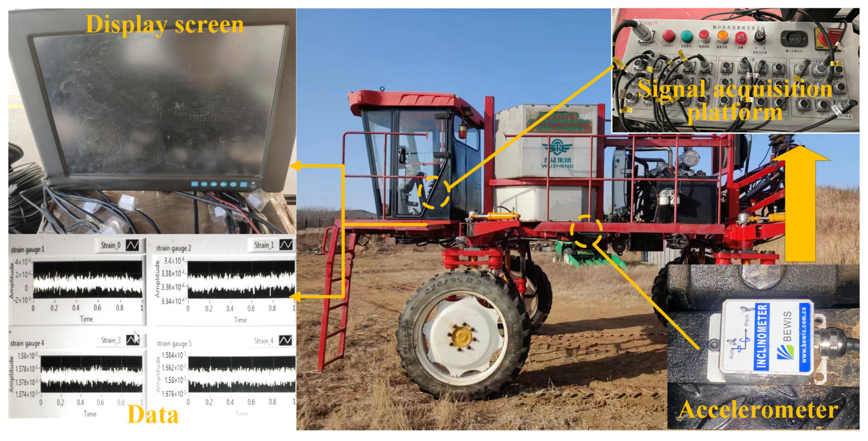
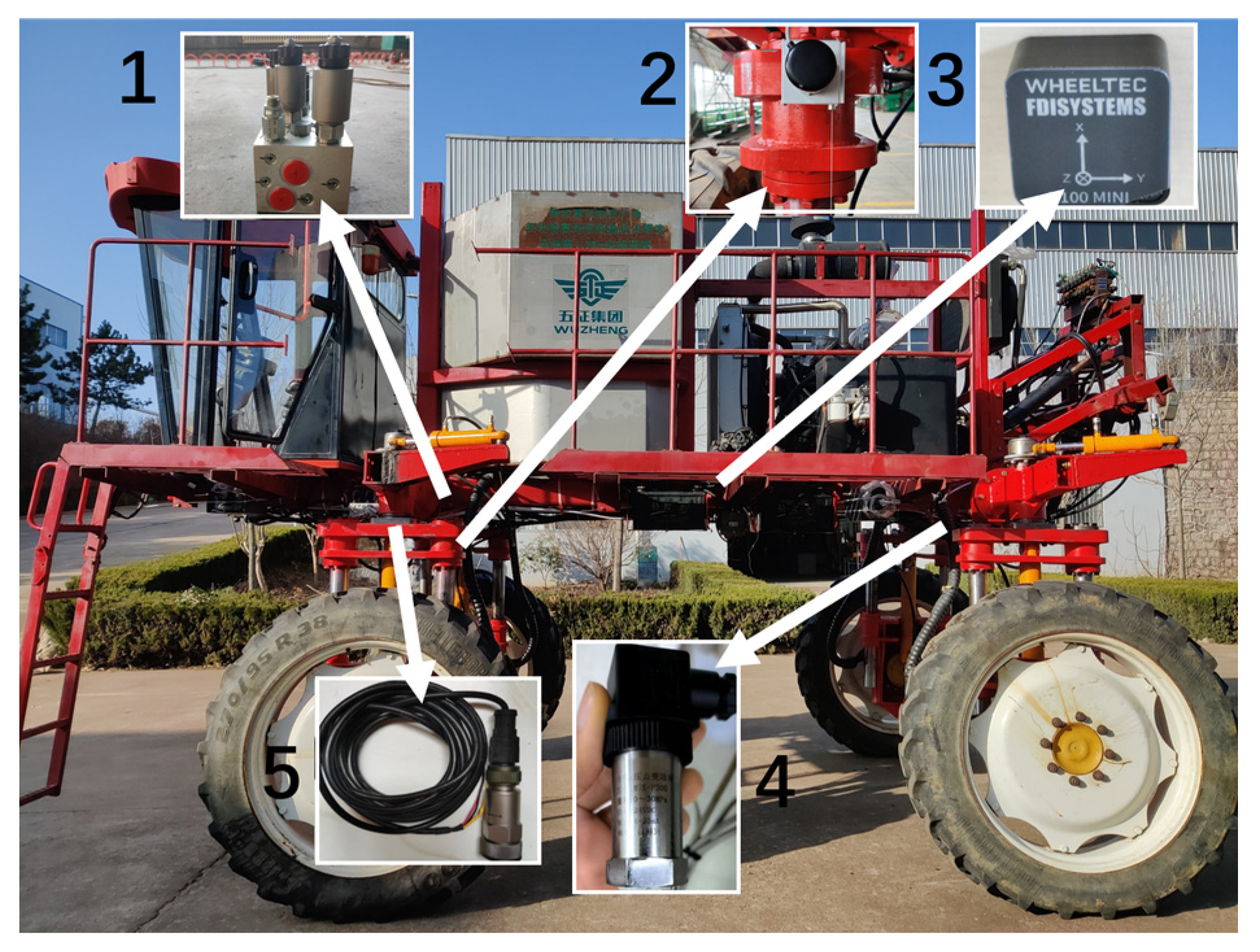
To guarantee accurate control, a three-axis acceleration sensor was installed at the center of mass of the large sprayer. The real vehicle data gathered during field transportation were utilized as training samples, with the T-S fuzzy controller being trained and optimized in MATLAB R2020b (Version R2020b, MathWorks Inc, Natick, MA, USA), taking into account the aforementioned evaluation function.

2.2.3. FNN Cooperative Controller Based on the AFSA-BP Algorithm

The contradiction between the steady-state error and the fuzzy rules is effectively mitigated by real-time adjustment of the fuzzy domain of the T-S controller via the variable universe. The traditional approach to determining the expansion factor often renders it challenging to precisely control the convergence speed, and the domain lacks clarity, thereby hindering the achievement of satisfactory practical application results. Fuzzy neural networks, as a type of network that constructs local approximations grounded in fuzzy systems, offer a guarantee for the convergence speed and accuracy of the algorithm, due to the physical meanings associated with their initial values.

(1)

Design of the FNN controller

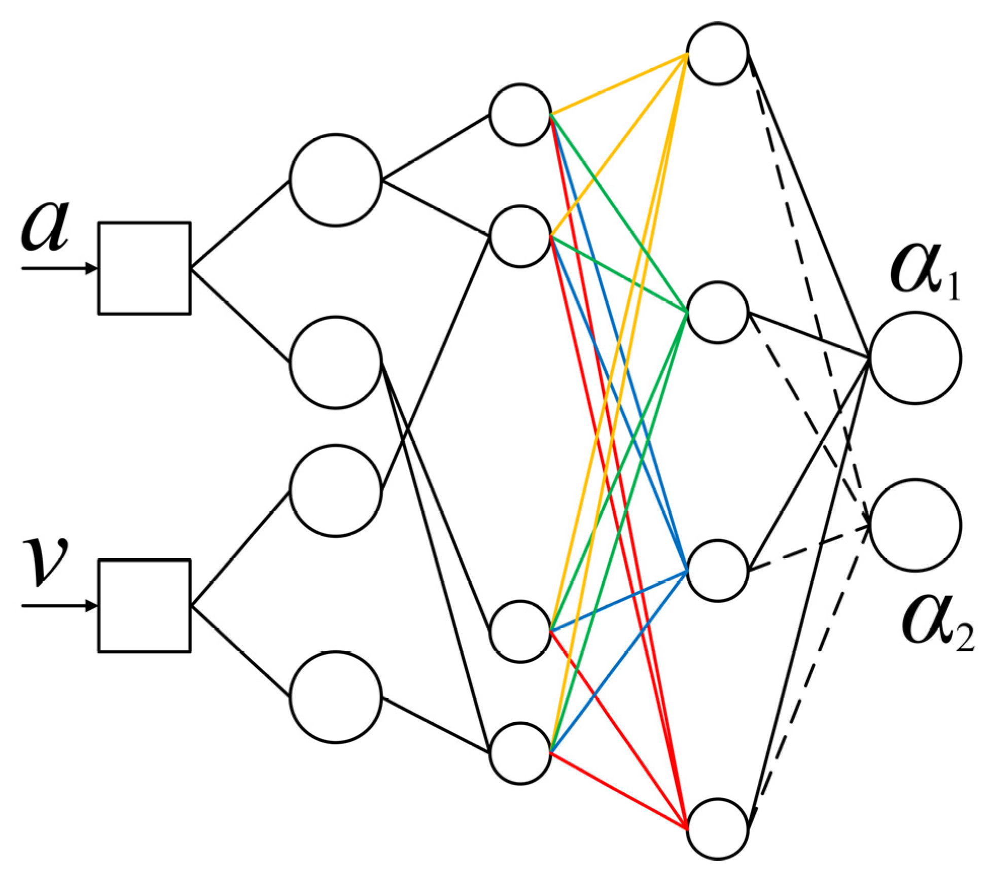
With the acceleration of the spring mass and the suspension dynamic deflection taken as the node inputs of the fuzzy neural network, the expansion and contraction factors α₁ and α₂ of the variable universe are outputted, being processed through seven fuzzy subsets, as shown in Figure 6.

In Figure 6, the first layer serves as the input layer, taking the sprung mass acceleration data and the Kalman filter’s estimated value as its input, namely x = [a_b, v_b]^T. The second layer is a fuzzy layer, employing a Gaussian function as its membership function b_ij. The third layer, being the rule layer, calculates the fitness c_j of each fuzzy rule. The fourth layer, known as the defuzzification layer, utilizes the area center of gravity method to realize defuzzification through d_j. Lastly, the fifth layer is the output layer, calculating and outputting the expansion and contraction factors α₁ and α₂ of the variable universe, with the result denoted as e_i. Specifically, each node in the third layer represents a fuzzy rule and functions to match the antecedent of the fuzzy rule, calculating the utility of each rule. The second layer has two groups of membership functions, and one membership function is selected from each group without repetition to form a combination, which then becomes a node in the third layer. For a given input, only the linguistic variable values near the input point have a higher membership value, while those further away from the input point have a very small membership value (for Gaussian membership functions) or zero (for triangular membership functions). The number of nodes in the fourth layer is the same as that in the third layer, and it performs normalization calculations on the applicability of each rule. The fifth layer is the output layer, which performs defuzzification calculations. The calculation formula is shown in Equation (13) [32].

$$\left\{\begin{array}{l}{b}_{ij}=\exp \left({\left(x_i-c_{ij}\right)}^2/{\sigma }_{ij}^2\right) , \left(j=1,2,\cdot \cdot \cdot ,b_1\right)\\ c_j={\mu }_1^j{\mu }_2^j\cdot \cdot \cdot {\mu }_n^j , \left(j=1,2,\cdot \cdot \cdot ,c;c={\displaystyle \prod _{i=1}^n{b}_1}\right)\\ d_j=c_j/{\displaystyle \sum _{i=1}^m{c}_j}\\ e_i={\displaystyle \sum _{j=1}^m{w}_{ij}\cdot d_j}\end{array}\right.$$

(13)

where c_ij is the center of the membership function; σ_ij is the width of the membership function; b₁ is the number of fuzzy partitions of the i-th (i = 1,2) input; w_ij is the weight of the i-th output of the layer j node.

c_ij, σ_ij, and w_ij are unknown parameters. By adjusting the numerical values of these three unknown parameters, the training effectiveness of the FNN algorithm for improving the variable universe expansion factors α₁ and α₂ is enhanced.

(2)

Optimization of Fuzzy Neural Networks via the AFSA-BP Algorithm

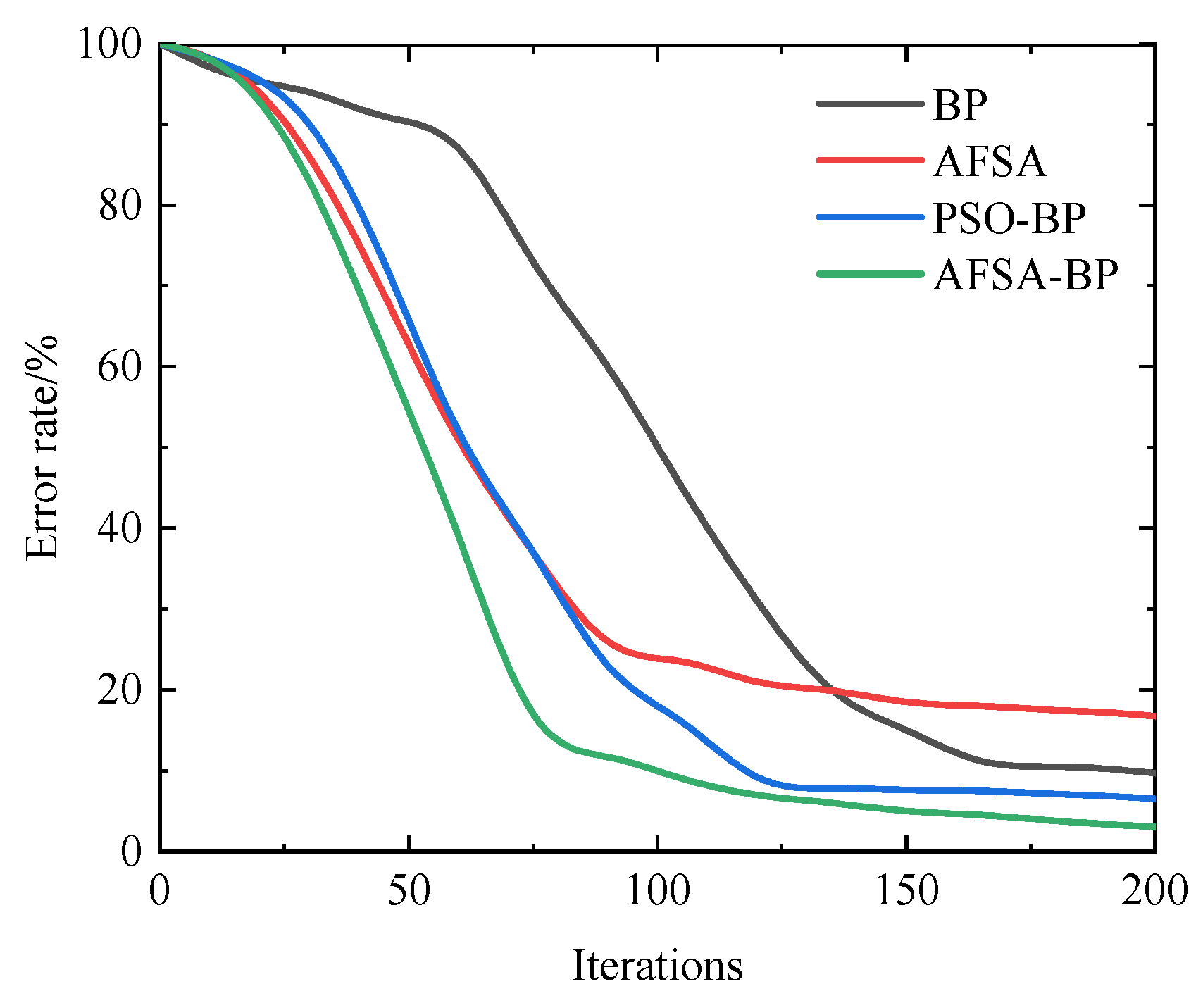
The FNN algorithm faces challenges in achieving optimal training results for the T-S fuzzy controller due to a vast number of undetermined parameters. Relying on empirical methods to set initial parameters significantly increases the algorithm’s calculation error, and its control accuracy is comparable to traditional mathematical function methods for determining the expansion and contraction factors, rendering FNN training redundant. To enhance the training effectiveness of the FNN algorithm, the AFSA algorithm is introduced to provide a more precise initial value for the BP algorithm. As a multi-objective optimization algorithm, the AFSA algorithm can conduct a global search for optimization targets without relying on the selection of the initial value. This characteristic complements the fast convergence of the BP algorithm, thus avoiding the issue of the AFSA algorithm being criticized for its difficulty in convergence during traditional multi-objective optimization processes. Specifically, the AFSA algorithm is integrated into the network to iteratively determine the center c_ij, width σ_ij, and weight w_ij of the optimal membership function. These values are then used as the initial parameters for the FNN algorithm. Subsequently, the BP algorithm is trained to enable the fuzzy neural network to rapidly approximate the ideal value.

By integrating the AFSA algorithm with the BP algorithm, this study leverages the global search capability of the AFSA algorithm in the initial optimization phase to swiftly approximate the Pareto front for the undetermined parameters of the FNN. In the subsequent training phase, the BP algorithm is employed to enhance convergence speed and optimize the search effectiveness within local solution sets. Incorporating the AFSA algorithm in the initial iteration stages addresses the issue of uncertain initial values for the BP algorithm, thereby improving training stability. The advantages of both algorithms throughout the iterative process result in outstanding theoretical performance throughout the entire training cycle.

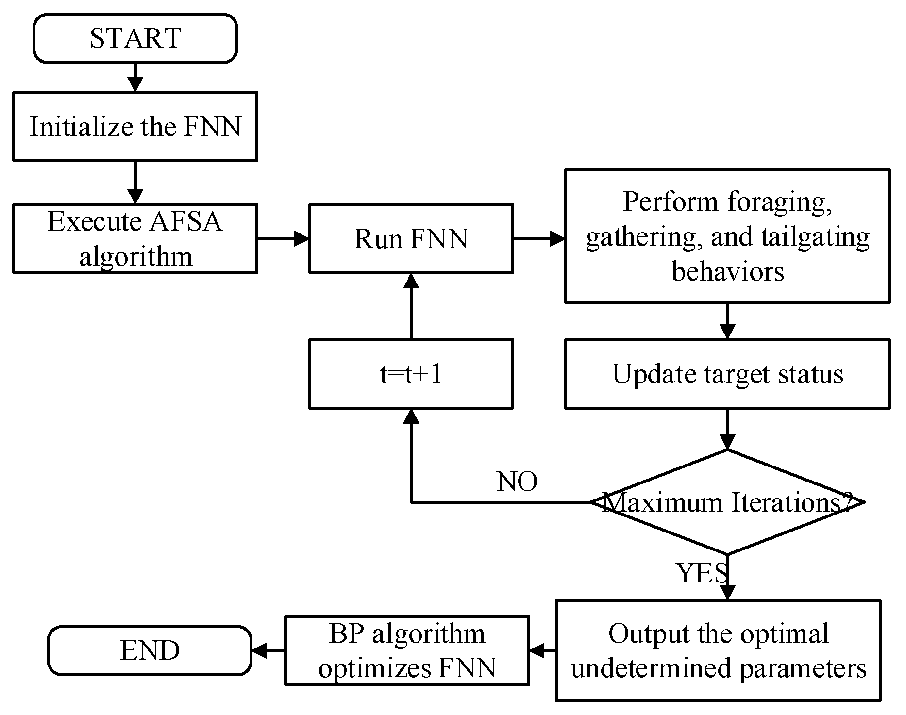
To mitigate the BP algorithm’s heavy reliance on initialization parameters, the AFSA algorithm, renowned for its robust global search capabilities and resilience to initial parameters, is introduced in the initial training phase. The AFSA algorithm categorizes fish schools into four distinct behavioral patterns: foraging, crowding, tailgating, and random behavior. The actual implementation proceeds as follows:

Step 1: A population N, the initial position of an artificial fish, a visual field V of that artificial fish, a step length step, a crowding factor γ, and a repetition number Try are initialized.

Step 2: Each artificial fish performs tail chasing, foraging behavior, and crowding and foraging behavior. If the outcome of executing any of these behaviors is superior to the original state, the artificial fish’s status is updated. If none of the behaviors result in an improved state, a random behavior is executed.

Step 3: The optimal positions of all artificial fish in the current iteration are recorded. If the maximum number of iterations is reached, the global optimal solution is outputted.

The update rules for the four typical behaviors [23] are as follows:

$$\left\{\begin{array}{l}{X}_{next}=X_i+\frac{X_j-X_i}{‖X_j-X_i‖}step\times rand\left(0,1\right)\\ X_{next}=X_i+\frac{X_c-X_i}{‖X_c-X_i‖}step\times rand\left(0,1\right)\\ X_{next}=X_i+\frac{X_{\max }-X_i}{‖X_{\max }-X_i‖}step\times rand\left(0,1\right)\\ X_{next}=X_i+\left(2\times rand\left(1,length(X_i)\right)-1\right)\times V\end{array}\right.$$

(14)

Assuming that the artificial fish’s current state is X_i, during foraging, a random state X_j within its field of vision is selected. The central position X_c is determined for schooling behavior, and X_max represents the location where food concentration is high and the environment is uncongested for tailing behavior. If congestion is detected in any of these behaviors, the artificial fish’s response is to execute the foraging behavior.

Compared to traditional multi-objective optimization algorithms, the AFSA algorithm boasts several advantages. (1) Each artificial fish school retains only the current position without any additional information, which favors global search. (2) The movement distance of artificial fish is influenced by the step size, while other algorithms (such as PSO, FA, etc.) are not constrained by the movement length, which makes the convergence speed of the artificial fish swarm algorithm slow and avoids premature convergence, providing a basis for switching to the BP algorithm in the future. (3) The AFSA algorithm disentangles the updating rules of social and individual attributes of fish schools, preventing the combined influence of individual and global optima on the iteration process and enhancing population diversity. These characteristics can serve as effective initialization inputs for the BP algorithm.

After the initial value of the BP algorithm has been roughly determined by the AFSA algorithm, the training focus is shifted to the BP algorithm to converge the unknown parameters of the target algorithm. Assuming that e and e′ are the predicted and actual outputs of the BP algorithm, the error cost function E [33] is represented by Equation (15).

$$E=\frac{1}{2}{\left(e’-e\right)}^2$$

(15)

Therefore, the gradient descent method [33] is employed to represent c_ij, σ_ij, and w_ij as follows:

$$\left\{\begin{array}{l}{c}_{ij}\left(\lambda +1\right)=c_{ij}\left(\lambda \right)-\nu \frac{\partial E}{\partial c_{ij}}\\ {\sigma }_{ij}\left(\lambda +1\right)={\sigma }_{ij}\left(\lambda \right)-\nu \frac{\partial E}{\partial {\sigma }_{ij}}\\ w_{ij}\left(\lambda +1\right)=w_{ij}\left(\lambda \right)-\nu \frac{\partial E}{\partial w_{ij}}\end{array}\right.$$

(16)

The learning rate of v remains consistently above 0, and the initial value of the network structure is set as the optimization result obtained from the AFSA algorithm, thus enhancing optimization efficiency. The training process of the AFSA-BP algorithm is shown in Figure 7.

3. Results

3.1. Software Simulation Testing

To validate the effectiveness of the proposed algorithm and assess the vibration reduction capabilities of the vibration reduction system of large sprayers under simulated field conditions, in MATLAB R2020b, the vibration signals gathered by the three-axis acceleration sensor of the actual vehicle were employed as the training dataset, which was then utilized to optimize the variable universe T-S fuzzy controller, and served as input for refining the fuzzy neural network cooperative controller. The effectiveness of active vibration reduction control was tested through software simulations. Specifically, first, the construction of m-files for the AFSA-BP algorithm and the FNN algorithm was implemented using MATLAB R2020b software. Then, in MATLAB/Simulink, a suspension simulation model was established, based on Equations (1)–(5), (7) and (8) of this study. Finally, the T-S fuzzy controller was trained by integrating the algorithm with the suspension model.

At the same time, to verify whether the training effectiveness of the AFSA-BP algorithm meets the theoretical expectations, BP [34], PSO-BP [35,36], and AFSA algorithms were employed as benchmarks for training and optimizing the undefined parameters of the FNN controller. The Particle Swarm Optimization (PSO) algorithm stands as one of the most classical and commonly employed optimization algorithms, widely applied in areas such as neural network training and fuzzy control systems [37,38]. By comparing the AFSA algorithm with the PSO algorithm, one can effectively validate the superior performance of the AFSA algorithm during the initial stages of optimization. After numerous training iterations, a comparison of the error rates across various stages is depicted in Figure 8.

As shown in Figure 8, the error rates of the AFSA, BP, PSO-BP, and AFSA-BP algorithms are 18.1%, 10.3%, 8.5%, and 3.9%, respectively. Compared with the other three algorithms, the improvement in error rate exhibited by the AFSA-BP algorithm is significant. Due to the uncertainty of initial values, the BP algorithm suffers from poor convergence performance in the initial stages and lacks sufficient global optimization capabilities. Conversely, the AFSA algorithm remains unaffected by initial values and possesses strong global search abilities during early iterations. Similar to the AFSA-BP algorithm, the PSO-BP algorithm can also achieve global optimization in the initial stages and transition to local optimization later on. However, due to the limitations of the algorithm’s inherent characteristics, the PSO algorithm’s global search ability is inferior to the AFSA algorithm, resulting in a slower convergence rate and a higher final error convergence compared to the AFSA-BP algorithm. By enhancing training speed while avoiding local optima, the AFSA-BP algorithm verifies its practicality and effectiveness.

(1)

Simulation Test of Obstacle Excitation

The field pavement primarily consists of soil and stones. The vibration transmitted from the stones to the vehicle body via the tires directly impacts the performance indicators of the vehicle, including the acceleration of the car body’s center of mass, roll angle, and pitch angle. Random stones causing pavement bulges have a significant effect on the uniformity of spraying and driving stability [39,40]. To simulate the vibration reduction effect of the sprayer under instantaneous impacts, an obstacle excitation with a bulge height of 0.1 m and a length of 5 m was input to the simulation model, and the speed of the sprayer was set at 1 m/s. Under identical initial conditions and a simulation time of 20 s, the time-domain and frequency-domain response curves of the sprung mass acceleration were obtained by comparing the vibration reduction simulation effects of the T-S fuzzy controller trained with the BP algorithm and the passive suspension, as shown in Figure 9.

The time-domain and frequency-domain responses of the entire vehicle suspension system after inputting simulated obstacle signals are shown in Figure 9a and Figure 9b, respectively. Compared with the time-domain curves of other suspensions, the AFSA-BP&T-S fuzzy controller introduced in this study exhibits a marked reduction in the vertical vibration acceleration amplitude when confronted with instantaneous impact signals. It tends to reach a stable state more quickly and enables faster system convergence. From the frequency-domain curve, it can be observed that the main frequency range of all curves is mostly concentrated between 0 and 3 Hz. Among them, the main frequency of the passive suspension is roughly distributed between 1.5 and 2.5 Hz, while the main frequency of the system after active control is concentrated below 1 Hz. Additionally, the power spectral density (PSD) of the AFSA-BP&T-S fuzzy controller is smaller. This indicates that the simulation conditions for obstacle excitation align with the operation environment in fields, where low-frequency vibrations are prevalent. The AFSA-BP&T-S controller provides effective control in vibration reduction across various frequency bands, especially exhibiting a significant suppression effect on low-frequency vibrations ranging from 0 to 3 Hz. It can effectively cope with strong uncertainties in random field excitations, such as road bumps, thereby enhancing driving comfort significantly.

On the premise of ensuring the overall effectiveness of active vibration reduction, the T-S fuzzy controller, utilizing the AFSA-BP algorithm, prioritizes enhancing the mitigation of low-frequency vibrations. It fulfills the fundamental requirements for farmland operations and validates the efficacy of the controller in regulating vibrations throughout large sprayers.

Similarly, when the same excitation is applied to the vehicle’s roll and pitch dynamics model, the resulting time-domain and frequency-domain simulation curves for pitch angle acceleration and roll angle acceleration are compared and shown in Figure 10.

As depicted, the time-domain and frequency-domain curves of pitch angle acceleration are shown in Figure 10a,b, while the time-domain and frequency-domain curves of roll angle acceleration are shown in Figure 10c,d, accordingly. As seen in Figure 10, although the effect of obstacle excitation on the vehicle’s body roll is not significant, the T-S fuzzy controller using the AFSA-BP algorithm excels substantially in managing both roll and pitch accelerations compared to the other two types. The main frequency of pitch angle acceleration in the passive suspension is concentrated around 2 Hz, whereas after active control, the pitch angle acceleration’s main frequency is concentrated around 0.5 Hz. The peak value of the frequency-domain curve decreases significantly. To precisely quantify vibration reduction effects of both active and passive suspension systems, data from the first 10 s were collected and the peak-to-peak (ptp) values of the three vibration reduction methods were statistically analyzed, as shown in

Table 3. Comparison of simulation data.

Control Type	Sprung Mass Acceleration	Pitch Angle Acceleration	Roll Angle Acceleration
Passive Suspension	7.737	4.322	2.052
BP&T-S	6.188	4.083	1.218
	−20.0%	−5.5%	−40.6%
AFSA-BP&T-S	6.001	3.889	1.088
	−22.4%	−10.0%	−50.4%

.

According to Table 3, it can be observed that the algorithm proposed in this study exhibits favorable effects on vehicle vibration, pitch, and roll control under the ideal condition of neglecting external interference. Compared to passive suspension, the ptp value of its sprung mass acceleration is reduced by 22.4%, the pitch angle acceleration’s ptp value is reduced by 10.0%, and the roll angle acceleration’s ptp value is reduced by 50.4%. As Figure 11 illustrates, the dynamic performance is significantly improved by the algorithm proposed in this study. It not only enhances the driving comfort during field operations but also effectively mitigates unsafe factors resulting from severe roll and pitch conditions. When encountering sudden low-frequency-impact road conditions, this algorithm also exhibits good control effects. It is effectively handled for braking “nodding” and steering sideslip, reducing the driving risk associated with the vehicle suspension system, and improving the handling performance during field operations.

(2)

Class D road simulation testing

Using the simulated road excitation model established in Section 2.1 as the input, the excitation impact of Class D road is applied to the four wheels at a speed of 20 km/h. By comparing the performance of the passive suspension system with the active suspension system, the vibration reduction effect is analyzed and presented in Figure 12.

It is evident from Figure 12 that under random road excitation, the active suspension exhibits a significant vibration reduction effect with regard to the three indices: sprung mass acceleration, pitch angle acceleration, and roll angle acceleration. The RMS value, serving as the benchmark for assessing suspension performance, is derived from processing the aforementioned data, including the RMS values of sprung mass acceleration, pitch angle acceleration, and roll angle acceleration, as shown in

Table 4. Comparison of suspension performance indices under random road excitation.

Index	Passive Suspension	BP&T-S		AFSA-BP&T-S
	RMS	RMS	Improvement Rate	RMS	Improvement Rate
sprung mass acceleration/m·s−2	1.471	1.193	19.9%	1.066	28.5%
pitch angle acceleration/rad·s−2	1.535	1.275	16.9%	1.203	21.6%
roll angle acceleration/rad·s−2	0.430	0.097	77.4%	0.091	78.8%

.

According to Table 4, the BP&T-S algorithm and AFSA-BP&T-S algorithm have significantly improved in three dynamic performance indexes, compared to the passive suspension. Specifically, the AFSA-BP&T-S algorithm has reduced the sprung mass acceleration, pitch angle acceleration, and roll angle acceleration by 28.5%, 21.6%, and 78.8%, respectively, outperforming the BP&T-S algorithm’s reductions of 19.9%, 16.9%, and 77.4%. The simulation results obtained under random road input are consistent with those under obstacle excitation input, thus verifying the effectiveness of the AFSA-BP&T-S algorithm.

3.2. Field Performance Test of Vibration Reduction System

In an idealized simulation environment, many complex real-world operating conditions are inevitably overlooked, and the limitations of the modeling process consistently hinder an accurate assessment of the superior vibration reduction effect of the controller [41,42]. To achieve an optimal vibration reduction effect in practical operating environments and verify the reliability of simulation results as well as the practicability of the controller, in this study, an AFSA-BP & T-S fuzzy controller was implemented on the suspension system of a sprayer, and its vibration reduction effectiveness was compared to that of a sprayer equipped with a BP & T-S fuzzy controller, as well as to a sprayer with a passive suspension without any controller This sprayer used in this test is independently developed. The test platform is shown in Figure 13. In the figure, number 1 is the proportional control valve group (Doylepacific, Ningbo, China), 2 is the displacement sensor (Milont, Shenzhen, China), 3 is the IMU sensor (Wheeltec, Dongguan, China) at the center of mass, 4 is the hydraulic system’s oil pressure sensor (Asmik, Hangzhou, China), and 5 is the acceleration sensor (Zesain, Shanghai, China) at the suspension position. The specific specifications and parameters are shown in

Table 5. Suspension performance index comparison under random road excitation.

Name	Specifications and Models	Technical Specification
Proportional control valve group	0~24 V	250 bar, 60 L/min
Displacement sensor	24 V power supply, 0–5 V output	0~1000 mm
IMU sensor	N100 MINI	9-DOF
Acceleration sensor	DC24 V, output 1~5 V	±5 g
Pressure sensor	24 V power supply, 0–5 V output	0~30 MPa

. The suspension vibration reduction algorithms is changed through the algorithm burning process.

Taking the field transportation link as an example, the sprayer was positioned on a flat hard pavement in an open field, in order to mitigate the impact of the changes in pavement roughness on the test results due to disruption by the sprayer. With a conventional operating speed of 15 km/h, it traversed a straight line on the same designated road section for 50 s, employing various vibration reduction control methods. The IMU sensor located at the centroid position in Figure 3 was utilized to gather the vehicle body position signal, which was then transmitted to a computer for real-time data processing. During the operation of the hydraulic system, thermal energy is generated as a result of the conversion of pressure loss, volume loss, and mechanical loss, thereby causing an increase in oil temperature. The varying viscosity of oil at different temperatures gives rise to diverse wear conditions of hydraulic components, affecting the accuracy of each test result [43,44]. Consequently, after each test, the sprayer returns to the starting point and remains stationary for 60 s to minimize the impact of hydraulic system heating on the vibration reduction performance. Due to the inability to achieve precise control over vehicle speed and position during field operations, the results of the direct test outputs exhibit significant errors, preventing a comparative analysis of the effectiveness of different algorithms. Therefore, each type of algorithm was tested 20 times, respectively. Ultimately, the data from the test with the best environmental variable control and the highest similarity in vibration reduction curves under the same road section were extracted, processed, and designated as the output curve for that group. The results are shown in Figure 14.

Given the significant correlation between the numerical values of indicators and external environmental disruptions (such as road conditions, driving conditions, etc.), field test data are not amenable to horizontal comparisons with simulation data [45,46]. As shown in Figure 14, the curves for sprung mass acceleration, pitch angle acceleration, and roll angle acceleration are illustrated for different vibration reduction strategies. The suspension system with active control exhibits varying degrees of improvement in these accelerations, particularly the AFSA-BP & T-S fuzzy control algorithm, which demonstrates a superior vibration reduction effect. Due to the disparity between real-world road conditions and the simulation settings, comparing the improvement rates of these indices becomes more pertinent. As evident from

Table 6. Comparison of data from field vibration reduction test.

Control Type	Sprung Mass Acceleration		Pitch Angle Acceleration		Roll Angle Acceleration
	RMS	Improvement Rate	RMS	Improvement Rate	RMS	Improvement Rate
Passive Suspension	1.831	/	0.923	/	0.358	/
BP&T-S	1.667	9.0%	0.832	9.5%	0.275	23.2%
AFSA-BP&T-S	1.496	18.3%	0.708	23.3%	0.259	27.7%

, when compared to the passive suspension, the AFSA-BP & T-S fuzzy controller in this study improves the sprung mass acceleration, pitch angle acceleration, and roll angle acceleration by 18.3%, 23.3%, and 27.7%, respectively, based on the root mean square value. Conversely, the BP & T-S fuzzy controller achieves improvements of 9.0%, 9.5%, and 23.2% on the three evaluation indices, thus highlighting the necessity of introducing the AFSA algorithm to optimize the initial BP value.

Given the intricacies of the field environment, the active suspension’s vibration reduction efficacy in the field test is not as ideal as the simulation, yet the overall trend of the test and simulation results remains comparable. This shows that the variable universe T-S fuzzy controller based on the AFSA-BP training FNN algorithm has a good vibration reduction effect when dealing with the low-frequency vibration of the field road, and its performance is better than that of traditional control algorithms.

4. Conclusions

In this study, based on the typical working conditions of large high-clearance sprayers in the field, an innovative control method for an active vibration reduction system is proposed, taking the HPS of the sprayer as the research object. This method is closely related to the specific working conditions and load variations of agricultural machinery and addresses the issue of insufficient vibration reduction performance of existing large sprayers during transportation, thus facilitating the systematic guidance of the design and testing of the sprayer’s suspension system. The main conclusions are as follows.

(1) The active control method proposed in this study took the four-wheel independent HPS of a sprayer as the control model and a T-S fuzzy controller as the foundation. The method encompassed innovative control processes such as real-time field data acquisition, adjusting fuzzy control rules and partitions with a variable universe method, and regulating the precision of the T-S system through a fuzzy neural network training approach. By effectively integrating an optimization method that combined the artificial fish swarm algorithm with the BP neural network algorithm, a fuzzy neural network collaborative controller was established, utilizing real-time data input from the sprayer.

(2) Through the software simulation and the field performance test, it has been proven that the requirements for vibration reduction in large sprayers are met by the active vibration reduction controller. The sprung mass acceleration, pitch angle acceleration, and roll angle acceleration were reduced to 1.496 m/s², 0.708 rad/s², and 0.259 rad/s². Compared with passive suspension, these three indicators have increased by 18.3%, 23.3%, and 27.7%, respectively, and the vibration reduction effect was obviously better than that of the traditional passive suspension, and the trend of the field performance test effect is consistent with that of the software simulation. The feasibility of the algorithm was demonstrated, thereby providing a new reference for the research into active vibration reduction of agricultural machinery.

References

1. Li, J.; Li, Z.; Ma, Y.; Cui, H.; Yang, Z.; Lu, H. Effects of leaf response velocity on spray deposition with an air-assisted orchard sprayer. Int. J. Agric. Biol. Eng. 2021, 14, 123–132. [Google Scholar] [CrossRef]
2. Fabula, J.; Sharda, A.; Mishler, B. Quantification of self-propelled sprayers turn compensation feature utilization and advantages during on-farm applications. Precis. Agric. 2022, 23, 1675–1687. [Google Scholar] [CrossRef]
3. Feng, J.; Christian, M.; Zheng, S.; Sun, T.; Gao, D. Hierarchical control strategy for active hydro pneumatic suspension vehicles based on genetic algorithms. Adv. Mech. Eng. 2015, 7, 951050. [Google Scholar] [CrossRef]
4. Zhao, J.; Gu, Z.; Zhang, S.; Ma, X.; Zhu, Y.; Hu, K. Research and Optimization on the Mechanical Property of Mining Dump Truck’s Hydro-Pneumatic Suspension. J. Mech. Eng. 2015, 51, 112–118. [Google Scholar] [CrossRef]
5. Kwon, K.; Seo, M.; Kim, H.; Lee, T.; Lee, J.; Min, S. Multi-objective optimisation of hydro-pneumatic suspension with gas–oil emulsion for heavy-duty vehicles. Veh. Syst. Dyn. 2020, 58, 1146–1165. [Google Scholar] [CrossRef]
6. Küçük, K.; Yurt, H.; Arıkan, K. Modelling and optimisation of an 8×8 heavy duty vehicle’s hydro-pneumatic suspension system. Int. J. Veh. Des. 2016, 71, 122–138. [Google Scholar] [CrossRef]
7. Yang, L.; Wang, R.; Ding, R.; Liu, W.; Zhu, Z. Investigation on the dynamic performance of a new semi-active hydro-pneumatic inerter-based suspension system with MPC control strategy. Mech. Syst. Signal Process. 2021, 154, 107569. [Google Scholar] [CrossRef]
8. Karnopp, D.; Crosby, M.; Harwood, R. Vibration Control Using Semi-active Force Generators. J. Eng. Ind. 1974, 96, 619–626. [Google Scholar] [CrossRef]
9. Xu, C. Research on Control Method of Semi-Active Suspension with Solenoid Valve Damper under Discrete Impact Road Conditions. Master’s Thesis, Harbin Institute of Technology, Harbin, China, 2020. [Google Scholar]
10. Matthias, J. Vertical trajectory planning: An optimal control approach for active suspension systems in autonomous vehicles. Veh. Syst. Dyn. 2021, 60, 3788–3809. [Google Scholar] [CrossRef]
11. Meng, J.; Wang, Z.; Xu, R.; Li, D. Research on active suspension control of high-speed train based on fuzzy compound strategy. J. Syst. Simul. 2021, 33, 1554–1564. [Google Scholar] [CrossRef]
12. Chen, K. A new state observer-based vibration control for a suspension system with magnetorheological damper. Veh. Syst. Dyn. 2022, 60, 3127–3150. [Google Scholar] [CrossRef]
13. Pusadkar, U.; Chaudhari, S.; Shendge, P.; Phadke, S. Linear disturbance observer based sliding mode control for active suspension systems with non-ideal actuator. J. Sound Vib. 2019, 442, 428–444. [Google Scholar] [CrossRef]
14. Li, H.; Miao, Z.; Lee, E. Variable universe stable adaptive fuzzy control of a nonlinear system. Comput. Math. Appl. 2002, 44, 799–815. [Google Scholar] [CrossRef]
15. Nurmaini, S. Differential drive mobile robot control using variable fuzzy universe of discourse. In Proceedings of the 2017 International Conference on Electrical Engineering and Computer Science (ICECOS), Palembang, Indonesia, 22–23 August 2017; pp. 50–55. [Google Scholar] [CrossRef]
16. Li, M.; Yang, G.; Li, X.; Bai, G. Variable universe fuzzy control of adjustable hydraulic torque converter based on multi-population genetic algorithm. IEEE Access 2019, 7, 29236–29244. [Google Scholar] [CrossRef]
17. Zadeh, L. Outline of a new approach to the analysis of complex systems and decision processes. IEEE Trans. Syst. Man Cybern. 1973, 3, 28–44. [Google Scholar] [CrossRef]
18. Jang, J. ANFIS: Adaptive-network-based fuzzy inference system. IEEE Trans. Syst. Man Cybern. 1993, 23, 665–685. [Google Scholar] [CrossRef]
19. Zhao, Z.; Liu, S.; Wei, J.; Qin, F. Improved biological neural network approach for path planning of differential drive agricultural robots with arbitrary shape. Comput. Electron. Agric. 2024, 216, 108525. [Google Scholar] [CrossRef]
20. Wang, T.; Chen, B.; Zhang, Z.; Li, H.; Zhang, M. Applications of machine vision in agricultural robot navigation: A review. Comput. Electron. Agric. 2022, 198, 107085. [Google Scholar] [CrossRef]
21. Cao, Z.; Zheng, S. MR-SAS variable universe fuzzy control in steering situation based on wheelbase preview. Optik 2016, 127, 9496–9503. [Google Scholar] [CrossRef]
22. Wang, J.; Wen, Y.; Ye, Z.; Jian, L.; Chen, H. Convergence analysis of BP neural networks via sparse response regularization. Appl. Soft Comput. 2017, 61, 354–363. [Google Scholar] [CrossRef]
23. Li, X. A New Intelligent Optimization Method-Artificial Fish School Algorithm. Ph.D. Thesis, Zhejiang University, Hangzhou, China, 2003. [Google Scholar]
24. Liu, T. Research on Vehicle Body Attitude Compensation Control Based on Semi-Active Hydro-Pneumatic Suspension. Master’s Thesis, Jiang Su University, Zhenjiang, China, 2019. [Google Scholar]
25. Song, X.; Fang, Q.; Zha, Z.; Li, N. The active suspension control system of a 7 DOFs automobile using fuzzy reasoning. J. Hunan Univ. (Nat. Sci.) 2003, 30, 56–59. [Google Scholar] [CrossRef]
26. Guo, Y.; Ren, C. Research on vibration reduction of semi-active suspension system of quarter vehicle based on time-delayed feedback control with body acceleration. J. Low Freq. Noise Vib. Act. Control 2022, 41, 701–711. [Google Scholar] [CrossRef]
27. Du, H.; Wei, J. Parameters optimization of interconnected hydro-pneumatic suspension for road comfort and road-friendliness based on genetic algorithm. J. Vib. Shock 2011, 30, 133–138. (In Chinese) [Google Scholar] [CrossRef]
28. Dong, B. A study on optimal control for vehicle active suspension system using a whole vehicle model. Automot. Eng. 2002, 24, 422–425. (In Chinese) [Google Scholar] [CrossRef]
29. Sun, J.; Zhao, K. Adaptive neural network sliding mode control for active suspension systems with electrohydraulic actuator dynamics. Int. J. Adv. Robot. Syst. 2020, 17, 1729881420941986. [Google Scholar] [CrossRef]
30. Ma, C.; Chang, J.; Lin, D. Input forces estimation of beam structures by an inverse method. J. Sound Vib. 2003, 259, 387–407. [Google Scholar] [CrossRef]
31. Sun, Z.; Xu, H. Fuzzy-neural network basedon T-S model. J. Tsinghua Univ. (Sci. Technol.) 1997, 37, 77–81. [Google Scholar] [CrossRef]
32. Sun, H. The Research and Application of the Fuzzy Neural Network. Ph.D. Thesis, North China Electric Power University, Baoding, China, 2006. [Google Scholar]
33. Peng, J. Application of gradient arithmetic method in the artificial neural network. J. Hebei GEO Univ. 2000, 23, 270–276. [Google Scholar] [CrossRef]
34. Yue, D.; Shang, S.; Feng, K.; Wang, H.; He, X.; Zhao, Z.; Wang, D. Research on the Model of a Navigation and Positioning Algorithm for Agricultural Machinery Based on the IABC-BP Network. Agriculture 2023, 13, 1769. [Google Scholar] [CrossRef]
35. Lu, K.; Liang, J.; Liu, M.; Lu, Z.; Shi, J.; Xing, P.; Wang, L. Research on Transmission Efficiency Prediction of Heavy-Duty Tractors HMCVT Based on VMD and PSO–BP. Agriculture 2024, 14, 539. [Google Scholar] [CrossRef]
36. Yuan, G.; Yang, W. Study on optimization of economic dispatching of electric power system based on Hybrid Intelligent Algorithms (PSO and AFSA). Energy 2019, 183, 926–935. [Google Scholar] [CrossRef]
37. Shi, J.; Zhang, Y.; Sun, Y.; Cao, W.; Zhou, L. Tool life prediction of dicing saw based on PSO-BP neural network. Int. J. Adv. Manuf. Technol. 2022, 123, 4399–4412. [Google Scholar] [CrossRef]
38. Zhang, J.; Wang, Y.; Niu, F.; Zhang, H.; Li, S.; Wang, Y. Parameterization of Multi-Angle Shaker Based on PSO-BP Neural Network. Minerals 2023, 13, 929. [Google Scholar] [CrossRef]
39. Xu, X.; Sun, Y.; Tian, X.; Zhou, L.; Li, Y. A double-EKF orientation estimator decoupling magnetometer effects on pitch and roll angles. IEEE Trans. Ind. Electron. 2021, 69, 2055–2066. [Google Scholar] [CrossRef]
40. Kamal Mazhar, M.; Khan, M.J.; Bhatti, A.I.; Naseer, N. A novel roll and pitch estimation approach for a ground vehicle stability improvement using a low cost IMU. Sensors 2020, 20, 340. [Google Scholar] [CrossRef]
41. Amer, Y.A.; El-Sayed, A.T.; Ahmed, E.E. Vibration reduction of a non-linear ship model using positive position feedback controllers. Int. J. Dyn. Control 2022, 10, 409–426. [Google Scholar] [CrossRef]
42. Wang, L.; Liu, J.; Li, Y. The optimal controller design framework for PID-based vibration active control systems via non-probabilistic time-dependent reliability measure. ISA Trans. 2020, 105, 129–145. [Google Scholar] [CrossRef] [PubMed]
43. Song, Q.; Chen, Y. The analysis of high oil temperature and the study of control in hydraulic system. Mod. Mach. 2010, 02, 45–46. [Google Scholar] [CrossRef]
44. Yang, H.; Wang, C. Hazard, cause and prevention of hydraulic system overheating. Chin. Hydraul. Pneum. 2005, 10, 77–79. [Google Scholar] [CrossRef]
45. Peng, J.; Chu, L.; Fwa, T.F. Determination of safe vehicle speeds on wet horizontal pavement curves. Road Mater. Pavement Des. 2021, 22, 2641–2653. [Google Scholar] [CrossRef]
46. Sun, D.J.; Zheng, Y.; Duan, R. Energy consumption simulation and economic benefit analysis for urban electric commercial-vehicles. Transp. Res. Part D Transp. Environ. 2021, 101, 103083. [Google Scholar] [CrossRef]
Figure 1. Oil circuit diagram of active suspension system. (1) Accumulator; (2) proportional valve; (3) two-position two-way proportional valve; (4) adjustable throttle valve; (5) adjustable throttle valve; (6) proportional drop valve; (7) proportional lift valve; (8) overflow valve; (9) differential pressure reducing valve.
Agriculture 14 00811 g001
Figure 2. Dynamics model of a 7-degree-of-freedom (DOF) sprayer. The arrows represent coordinate system.
Agriculture 14 00811 g002
Figure 3. Field collection process for road surface information.
Agriculture 14 00811 g003
Figure 4. Workflow of active suspension.
Agriculture 14 00811 g004
Figure 5. Observation effect of Kalman filter. (a) Curve for estimating the sprung mass velocity; (b) curve for estimating the unsprung mass velocity.
Agriculture 14 00811 g005
Figure 6. Schematic diagram of the fuzzy neural network. Lines of the same color represent connections from the same node to the next network layer.
Agriculture 14 00811 g006
Figure 7. AFSA-BP algorithm workflow.
Agriculture 14 00811 g007
Figure 8. Comparison of algorithm errors.
Agriculture 14 00811 g008
Figure 9. Simulation effect of sprung mass acceleration under obstacle excitation. (a) Time-domain curve; (b) frequency-domain curve.
Agriculture 14 00811 g009
Figure 10. Simulation effect of pitch and roll under obstacle excitation. (a) Time-domain curve of pitch angle acceleration; (b) frequency-domain curve of pitch angle acceleration; (c) time-domain curve of roll angle acceleration; (d) frequency-domain curve of roll angle acceleration.
Agriculture 14 00811 g010
Figure 11. Acceleration attenuation rate under obstacle excitation.
Agriculture 14 00811 g011
Figure 12. Comparison of vibration reduction effect under Class D road. (a) Curve of sprung mass acceleration; (b) curve of pitch angle acceleration; (c) curve of roll angle acceleration.
Agriculture 14 00811 g012
Figure 13. Field test platform for the sprayer. (1) Proportional control valve group; (2) displacement sensor; (3) IMU sensor; (4) pressure sensor; (5) acceleration sensor.
Agriculture 14 00811 g013
Figure 14. Comparison of vibration reduction test effects in the field. (a) The curve comparison of sprung mass acceleration between an active suspension equipped with the AFSA-BP & T-S algorithm and a passive suspension. (b) The curve comparison of sprung mass acceleration between a suspension equipped with the BP & T-S algorithm and a passive suspension. (c) The curve comparison of pitch angle acceleration between an active suspension equipped with the AFSA-BP & T-S algorithm and a passive suspension. (d) The curve comparison of pitch angle acceleration between a suspension equipped with the BP & T-S algorithm and a passive suspension. (e) The curve comparison of roll angle acceleration between an active suspension equipped with the AFSA-BP & T-S algorithm and a passive suspension. (f) The curve comparison of roll angle acceleration between a suspension equipped with the BP & T-S algorithm and a passive suspension.
Agriculture 14 00811 g014