Article

Analyzing the Impact of Storm ‘Daniel’ and Subsequent Flooding on Thessaly’s Soil Chemistry through Causal Inference

by
Miltiadis Iatrou
1,*,
Miltiadis Tziouvalekas
2,
Alexandros Tsitouras
2,
Elefterios Evangelou
2,
Christos Noulas
2,
Dimitrios Vlachostergios
2,
Vassilis Aschonitis
1,
George Arampatzis
1,
Irene Metaxa
1,
Christos Karydas
3 and
Panagiotis Tziachris
1
1
Soil and Water Resources Institute, Hellenic Agricultural Organization “DIMITRA”, 57001 Thessaloniki, Greece
2
Institute of Industrial and Forage Crops, Hellenic Agricultural Organization “DIMITRA”, 41335 Larissa, Greece
3
Ecodevelopment S.A., 57010 Thessaloniki, Greece
*
Author to whom correspondence should be addressed.
Agriculture 2024, 14(4), 549; https://doi.org/10.3390/agriculture14040549
Submission received: 29 January 2024 / Revised: 26 March 2024 / Accepted: 27 March 2024 / Published: 30 March 2024
(This article belongs to the Special Issue Application of Machine Learning and Data Analysis in Agriculture)

Abstract

:
Storm ‘Daniel’ caused the most severe flood phenomenon that Greece has ever experienced, with thousands of hectares of farmland submerged for days. This led to sediment deposition in the inundated areas, which significantly altered the chemical properties of the soil, as revealed by extensive soil sampling and laboratory analysis. The causal relationships between the soil chemical properties and sediment deposition were extracted using the DirectLiNGAM algorithm. The results of the causality analysis showed that the sediment deposition affected the CaCO3 concentration in the soil. Also, causal relationships were identified between CaCO3 and the available phosphorus (P-Olsen), as well as those between the sediment deposit depth and available manganese. The quantified relationships between the soil variables were then used to generate data using a Multiple Linear Perceptron (MLP) regressor for various levels of deposit depth (0, 5, 10, 15, 20, 25, and 30 cm). Then, linear regression equations were fitted across the different levels of deposit depth to determine the effect of the deposit depth on CaCO3, P, and Mn. The results revealed quadratic equations for CaCO3, P, and Mn as follows: 0.001XCaCO32 + 0.08XCaCO3 + 6.42, 0.004XP2 − 0.26XP + 12.29, and 0.003XMn2 − 0.08XMn + 22.47, respectively. The statistical analysis indicated that corn growing in soils with a sediment over 10 cm requires a 31.8% increase in the P rate to prevent yield decline. Additional notifications regarding cropping strategies in the near future are also discussed.

Graphical Abstract

1. Introduction

According to recent reports, based on several years of observations by 27 national academies from the European Union (EU), Norway, and Switzerland, the frequency of extreme weather events, including hydrological events, has increased by 60% in Europe over the past three decades. The largest increase has been observed in hydrological phenomena, such as floods, landslides, and avalanches [1,2]. Also, severe summer and late-spring floods have occurred more frequently in the last few years in Greece. Global warming might cause periods of heavy precipitation in Europe during the summer, which may lead to more frequent floods, even though summers may become drier on average [3,4].
On 5–7 September 2023, Thessaly was hit by a once-in-a-1000-year weather event, where extreme rainfall (700 mm in 48 h) caused extensive floods. By 7 September 2023, less than 60 h after the rains started, 72,951 ha had been inundated by flooding (Figure 1). The flood led to land loss due to erosion and resulted in the accumulation of sediment in various areas across the Thessaly plain.
Storm ‘Daniel’ caused an extended sediment deposition in the flooded areas, which, in some cases, reached a 60 cm depth of deposit (Figure 2). Clearly, the 2023 crop season suffered significant impacts due to flooding. The floods destroyed annual crops just before the harvest period like cotton and corn, as well as other vegetable crops such as clover (mainly alfalfa), but also industrial tomato (i.e., the medium–late varieties). Permanent vine plantations and tree crops such as olives, apples, pears, almonds, pistachios, walnuts, peaches, kiwis, etc., also suffered extensive damage. Moving forward, it is crucial to educate farmers about the flood’s influence on soil chemistry. This is especially important because numerous fields experienced substantial soil deposition. Understanding these changes is key for effective management in the upcoming crop season.
Focusing exclusively on correlation analysis, in the context of the complex and multidimensional dataset that was derived from the soil analysis, introduces significant obstacles. It is imperative to unravel the causal links instead of depending on the correlations that might arise from the superficial associations among variables [5]. In essence, approaches that mainly concentrate on learning correlations to assess the influence of an environmental factor on soil quality often fall short in accurately capturing the real underlying dynamics. Statistical-based methods fail to reveal the direct and indirect causal connections in data. They also face challenges in identifying and adjusting for potential biases [6]. In recent years, machine learning (ML) has been extensively used in processing complex data, like environmental or soil data, thereby aiding in decision making and forecasts [7,8]. However, the effectiveness of these prediction models in environmental contexts is dependent on the dataset size. If there are not enough data available, then the models do not generalize well in varied settings. A key issue is that ML models often capture non-causal links between inputs and outputs, thereby leading to reduced effectiveness in different environments [9].
Conducting controlled experiments is an effective way to identify and understand causal mechanisms for various natural phenomena [10]. However, performing controlled experiments is often impossible and expensive. Causal inference in general has become increasingly important in medicine and social science as, in many cases, it is ethically impossible to experiment, discover, or understand the causal mechanisms of the various factors affecting life [10]. Causal machine learning may likely play a significant role in the field of environmental sciences, particularly in considering the complexity of the variables affecting the nutrient availability in soil, the high dimensionality of soil data, and the extensive nature of agriculture. To estimate the causal effect of sediment deposit on soil chemical properties, directed acyclic graphs (DAGs) were employed to delineate the potential causal connections among variables, thereby aiding in creating a more universally applicable prediction model for the effect of sediment deposit on the chemical properties of soil. Fehr [9] suggested that prediction accuracy improves in diverse settings when the models are based on causal factors rather than on the resultant elements of the predicted variable. Causal machine learning (CML) introduces a deeper layer of comprehension to the system, thereby enhancing the general applicability and explicability of existing ML frameworks [6].
A major challenge with employing machine learning and deep learning methods is the lack of interpretability in how outcomes are derived, as highlighted by Prendin [11]. Typically, the selection of models is based on their predictive accuracy following the adjustment of hyperparameters. Nonetheless, in the context of agriculture, where models inform decision making, it is essential for these algorithms to be comprehensive and interpretable. Interpretability refers to the extent to which the rationale behind a model’s decisions can be understood. To address the opacity of complex models, various tools have been developed in recent years to shed light on the workings of black box models. One such tool is Shapley Additive Explanation (SHAP) analysis, an approach that is grounded in game theory and quantifies the contribution of each feature to the model’s prediction through the computation of Shapley values [12,13]. This involves systematically altering the input data across all observations and features, while keeping the dataset otherwise unchanged, to isolate the effect of each feature [14,15]. In this research, we adopted an innovative approach through constructing a causal model that uses techniques for causal inference, and we evaluated its reliability with a machine learning algorithm paired with an interpretability mechanism like SHAP. The consistency in results from both the causal and interpretative analyses allowed for an increased confidence in the outcomes, thereby emphasizing that precise feature interpretation is crucial for the model in recommending effective management strategies for crop fertilization. While correlation analysis is the most popular statistical tool used to understand the relations among soil variables, it is not appropriate in the context of this study because our objective extends beyond not only examining the relationships between the soil variables, but also exploring whether sediment deposit causes change in the soil chemistry [16]. To strengthen the foundation of our study, we used the current advancements of causal inference along with ML. By integrating these two methods, our study contributes to the application of causal inference and ML in environmental applications.
The objectives of the current work are twofold: firstly, to quantitatively assess the causal effects of sediment deposition on key soil chemical parameters such as CaCO3, P, and Mn levels; and, secondly, to develop management strategies to mitigate the potential yield losses in crops due to altered soil chemistry.

2. Materials and Methods

A combination of Copernicus Sentinel satellite images (European Space Agency, Paris, France), i.e., Sentinel-1 and Sentinel-2, was utilized for monitoring the flood [17]. Sentinel-1 is a radar satellite mission designed to provide all-weather, day-and-night imaging capabilities. It is particularly useful for monitoring natural disasters like floods as it can penetrate cloud cover and gather data on surface conditions. Sentinel-2 is a multispectral imaging satellite mission designed to provide high-resolution optical imagery. It can capture detailed visual information about the Earth’s surface. A combination of the radar data from Sentinel-1 and optical imagery from Sentinel-2 offered a comprehensive view of the flood-affected regions. These Copernicus Sentinel satellites are part of the European Union’s Copernicus Earth Observation program, which aims to provide accurate and timely information for environmental monitoring, emergency response, and other Earth observation applications. The use of both radar and optical satellite data allows for a more thorough analysis of the flood event, encompassing both the physical presence of the water and the visual changes in the landscape caused by the inundation. Monitoring via satellite imagery for identifying and delineating the affected areas revealed that severe inundation occurred in the Karditsa, Larissa, and Lake Karla areas, as shown in Figure 1. The flood caused an extended sediment deposition in the flooded areas, as shown in Figure 2.

2.1. Soil Sampling and Analysis

Composite soil samples (i.e., three subsamples from a 1 × 1 m surface area were mixed to make a composite soil sample) were extracted to a depth of 30 cm from 321 locations in the area that was impacted by the flooding. Immediately after the floodwaters receded, the soil samples were collected from the surface at each site. Out of these, 217 samples originated from areas without any sediment coverage, while 104 samples were gathered from fields with sediment layers varying between 1 and 60 cm in depth. The soil samples were air-dried and sieved following standard procedures. The soil samples were analyzed for soil fertility (macro and micro-elemental analysis) and other basic soil physicochemical parameters with standard internationally recognized methods at the accredited laboratory of Soil, Plant and Water analyses of the Institute of Industrial and Forage Crops of the Hellenic Agricultural Organization “DIMITRA”. The analysis assessed 18 soil parameters, including the weight percentage of sand, clay, and silt, as well as the soil pH, electrical conductivity (EC), soil organic matter content (SOM), calcium carbonate content (CaCO3), organic carbon (C), total nitrogen (N), phosphorus (P), potassium (K), sodium (Na), magnesium (Mg), iron (Fe), zinc (Zn), manganese (Mn), copper (Cu), and calcium (Ca) levels. The pH and EC values were measured using a soil-to-water ratio of 1:1 with specific meters [18,19]. Total nitrogen was quantified via the Kjeldahl technique [20], while C and SOM were determined by the Walkley–Black method [21]. The CaCO3 content was assessed by titration [22], and the soil texture was evaluated using the Bouyoucos hydrometer approach [23]. The Olsen method was employed for P [24]. The ammonium acetate extraction method, followed by an atomic absorption spectrophotometer reading, was used for Na, K, Ca, and Mg [25]. Additionally, Mn, Cu, Fe, and Zn were extracted using DTPA and quantified with an atomic absorption spectrophotometer [26].

2.2. Data Preprocessing

The dataset that was analyzed to assess the impact of sediment on soil chemistry, after excluding the missing data, comprised 296 entries. The dataset was randomly divided into a training set (80%, or 237 entries) and a test set (20%, or 59 entries). To reduce dimensionality and filter out insignificant attributes, the random forest algorithm was employed [27]. This step led to the exclusion of variables deemed of low importance based on the feature importance scores derived from the random forest model [28]. The remaining variables from the initial set were then examined for collinearity using Spearman’s rank correlation. Features that were found to be less critical by the random forest model and did not significantly increase error rates were removed [29].

2.3. Machine Learning

A LightGBM regressor was utilized to establish a relationship between the soil deposit depth and the soil variables [30]. Table 1 provides definitions for the soil variables, which serve as input features for the LightGBM model. The LightGBM algorithm was used to identify the relative importance of each variable on deposit depth. The LightGBM regressor was selected as it is a dynamic ML technique delivering state-of-the-art results in the ML framework [31]. Introduced by Microsoft in 2017, LightGBM is an advanced optimization model algorithm that builds on the gradient-boosted decision tree framework. It represents an enhancement over XGBoost [32] by offering more efficient parallel training, reduced memory usage, and improved accuracy. Utilizing a histogram-based decision tree algorithm, LightGBM transforms weak learners into strong ones. The key advantage of this technique is that it provides a refined sample splitting approach that minimizes the risk of overfitting. Additionally, its gradient-based, one-side sampling (GOSS) is an innovative feature. GOSS prioritizes samples with larger gradients while randomly selecting those with smaller gradients, thereby enhancing the algorithm’s efficiency and accuracy [30]. The LightGBM algorithm depends a great deal on the optimal selection of hyperparameters; thus, despite it uses the gradient boosting framework, which is prone to overfitting, it is a very efficient algorithm. The Optuna library was used for the hyperparameter tuning of the LightGBM algorithm [33]. A total of 100 trials with different combinations of hyperparameters were tested, and the combination of parameters that minimized the Mean Absolute Error (MAE) was selected. The optimum hyperparameter values for the LightGBM model were as follows: learning_rate = 0.02, num_leaves = 662, subsample = 0.2, colsample_bytree = 0.63, and min_data_in_leaf = 15.

2.4. SHAP Analysis

To elucidate the factors related to deposit depth, as determined by the LightGBM model, Shapley Additive Explanation (SHAP) analysis was implemented [12,13]. Linear regression models are more easily explainable, yet they fall short in capturing the complex, nonlinear relationships within data. In contrast, more complex algorithms are more capable in capturing nonlinear patterns, but they present greater challenges in terms of interpretability [34]. For this study, the SHAP method was selected due to its ability to deliver a detailed assessment of feature significance. SHAP, an Explainable Artificial Intelligence (XAI) approach, draws from game theory and quantifies a feature’s effect on a model’s output [14,15]. It calculates a Shapley value for each prediction by altering the input data across all rows for one feature per test, while keeping the remaining data consistent with the original. Each SHAP value, thus computed individually for every prediction, elucidates that specific prediction. It does so by assessing the deviation from the model’s forecast to that obtained by altering a single feature. A significantly positive sum of these deviations suggests a strong positive influence of the feature on that prediction. Conversely, a highly negative sum indicates a negative influence, while a sum near zero implies the feature’s minimal impact. Practically, SHAP constructs a small explainer model for each observation, thereby explaining the rationale behind the model’s prediction for that case [35]. This is especially useful for nonlinear methods like LightGBM. While this algorithm is effective in reducing prediction errors, discerning the logic behind their outputs is often challenging. For visualization purposes, the SHAP library was utilized to create graphical representations of feature importance and SHAP dependency plots.

2.5. Casual Representation, Discovery, and Reasoning

Causal models offer insights into the generative processes involved in the creation of the data by going beyond the mere correlations between the variables [36]. Causal representation involves an understanding of the causal relationship between the variables. Causal discovery is the process of discovering the causal links between the variables, while causal reasoning focuses on estimating the impact of the interventions between the variables [6]. In DAGs, each node symbolizes a variable, while the directed edges indicate direct causal influences, with the arrow pointing from the cause to its subsequent effect [9,37]. A DAG was employed to map the causal connections among the variables. Initially, the Direct Linear non-Gaussian Acyclic Model (DirectLiNGAM) was employed to map the causal links between the variables. The DirectLiNGAM algorithm is an improvement on the LiNGAM algorithm as it can more robustly estimate the causal structure in the data if the data do not strictly meet the non-Gaussianity assumption of the original LiNGAM algorithm. DirectLiNGAM assumes that the actual causal connection in the data is linear, acyclic, and without any hidden confounders. It also introduces an improved method for estimating the causal order in the variables, which is characterized by the following three key steps: pairwise causality tests, the estimation of the causal ordering based on the pairwise tests, and the estimation of the connection strengths. In general, the assumption of non-Gaussianity (data that are non-Gaussian-distributed) enables the LiNGAM algorithm to extend beyond second-order statistical analysis, such as covariance, to fully uncover the causal structure within the data [10,16,38].
Subsequently, Regression with Subsequent Independence Test (RESIT) was employed to illustrate the impact of sediment deposition on the soil chemistry. Proposed by Hoyer et al. [39] and Peters et al. [40], RESIT is recognized as a method for non-linear causal discovery, and it is capable of discerning causal structures under the assumption of non-linearity. The RESIT method is based on the principle that if X causes Y, then, after regressing Y on X, the residuals should be independent of X. There are three steps in this procedure: a regression is performed between Y and X to predict Y based on X, the residuals representing the part of Y not explained by X are computed, and a kernel-based conditional independence test is performed between X and the residuals [41]. For this study, the RESIT algorithm was incorporated with a Multiple Linear Perceptron (MLP) regressor for its implementation instead of a simple linear regression as MLP is a non-linear model and particularly useful for complex data coming from soil analysis. The RESIT algorithm can make use of any regression model for regressing each of the variables with all the other variables for the purpose of finding the causal link [40]. However, for this specific study, it was found that the RESIT model, when the MLP regressor was included as part of its regression mechanism, yielded the best results. The confidence level for the different deposit depths was obtained by bootstrapping the dataset 10 times using the multiscale bootstrap method. The multiscale bootstrap method gives unbiased p-values with much higher statistical reliability [42]. For the MLP regressor, the data were scaled using the standard scaler (scaled = (x − μ)/σ, where μ is the mean, and σ is the standard deviation from the mean). The MLP model was configured with the maximum iteration parameter set to 500. This parameter defines the maximum number of epochs over the data before the training process is halted. This hyperparameter is crucial for controlling the training time and preventing overfitting [43,44]. An MLP is a class of feedforward artificial network (ANN) that consists of at least three layers of nodes: an input layer, one or more hidden layers, and an output layer. The hidden_layer_sizes hyperparameter defines the size and number of the hidden layers. For this architecture, two configurations were considered for tuning: a two-layer configuration where each layer consisted of 10 neurons, and a three-layer configuration with each layer also consisting of 10 neurons. Finally, the optimum architecture included a three-layer configuration for the hidden layers. Data were evaluated using the bootstrap approach with n_sampling = 10, which allowed examining the generated causal effects through confidence intervals. Following this, data were generated based on the causal relationships of the soil data. A MLP regressor was used to fit the causal data generator, which produced datasets for varying sediment deposit depths (0, 5, 10, 15, 20, 25, and 30 cm). Then, linear regression equations were fitted to determine the trends of increase in the CaCO3 and Mn, as well as the decrease in P, in relation to these deposit depth levels.
Cadmium, lead, zinc, and nickel were measured but were not found to be higher compared to the soils without sediments, and they were also not found in higher-than-normal levels; for this reason, they were not included in the causal inference analysis.
The entire process, encompassing data analysis, model development, and visualization, was conducted using Python [45] with tools like Matplotlib and seaborn aiding in visualization creation [46,47]. The lingam library was used for performing the DirectLINGAM [10,38] and RESIT algorithms [40]. An overview of the analysis pipeline and processes is presented in Figure 3.

3. Results

3.1. Causal Inference

The soil analysis showed a significant impact of sediment depth on the soil chemical properties. In addition, a Spearman’s test showed a significant positive correlation between deposit depth and CaCO3 (p < 0.001), Mn (p < 0.001), Fe (p < 0.001), Cu (p < 0.007), and pH (p < 0.009), as well as a negative correlation with K (p < 0.004). Indeed, as demonstrated in the histograms of Figure 4, elevated levels of Cu, Fe, and Mn were predominantly found in the soil deposits. Causal data analysis suggested that the deposit depth affects the CaCO3 content in soil chemistry, there is a causal link between Mn and deposit depth, as well as that a causal link exists between CaCO3 with P and Fe (Figure 5). The DAG, as shown in Figure 5, also showed that the deposit depth affected the physical properties of the soil, thereby leading to an increase in sand content and a reduction in the ratio of organic carbon to total nitrogen content. Some estimated relationships, however, were controversial to the domain knowledge, as, for example, the causal link between CaCO3 and P clearly went in the opposite direction. This was also clearly true for the causal link between Mn and the deposit depth, as the deposit caused Mn to increase, while the DAG shows the opposite.
The RESIT algorithm was used to obtain the confidence level for the various sediment depths. Figure 6a shows that, for deposit depths higher than 10 cm, CaCO3 increased significantly compared to the soils with no sediment deposit. Figure 6b additionally indicates that, for a deposit depth exceeding 20 cm, the P concentrations were significantly lower compared to soils without sediment. Figure 6c demonstrates that an increased deposit depth resulted in significantly higher Mn concentration, while Figure 6d shows that Fe levels were not affected by the soil deposit.
We generated data based on the causal relationships using an MLP regressor, which provided datasets for various levels of deposit depths (0, 5, 10, 15, 20, 25, and 30 cm). Polynomial equations showed that CaCO3 and Mn increased in relation to the sediment depths according to the following equations (Figure 7):
CaCO3 = 0.001XCaCO32 + 0.08XCaCO3 + 6.42,
Mn = 0.003XMn2 − 0.08XMn + 22.47.
Meanwhile, P decreased in relation to sediment depth according to the following equation:
P = 0.004XP2 − 0.26XP + 12.29.
However, the confidence intervals were only obtained by bootstrapping and are shown in Figure 6.

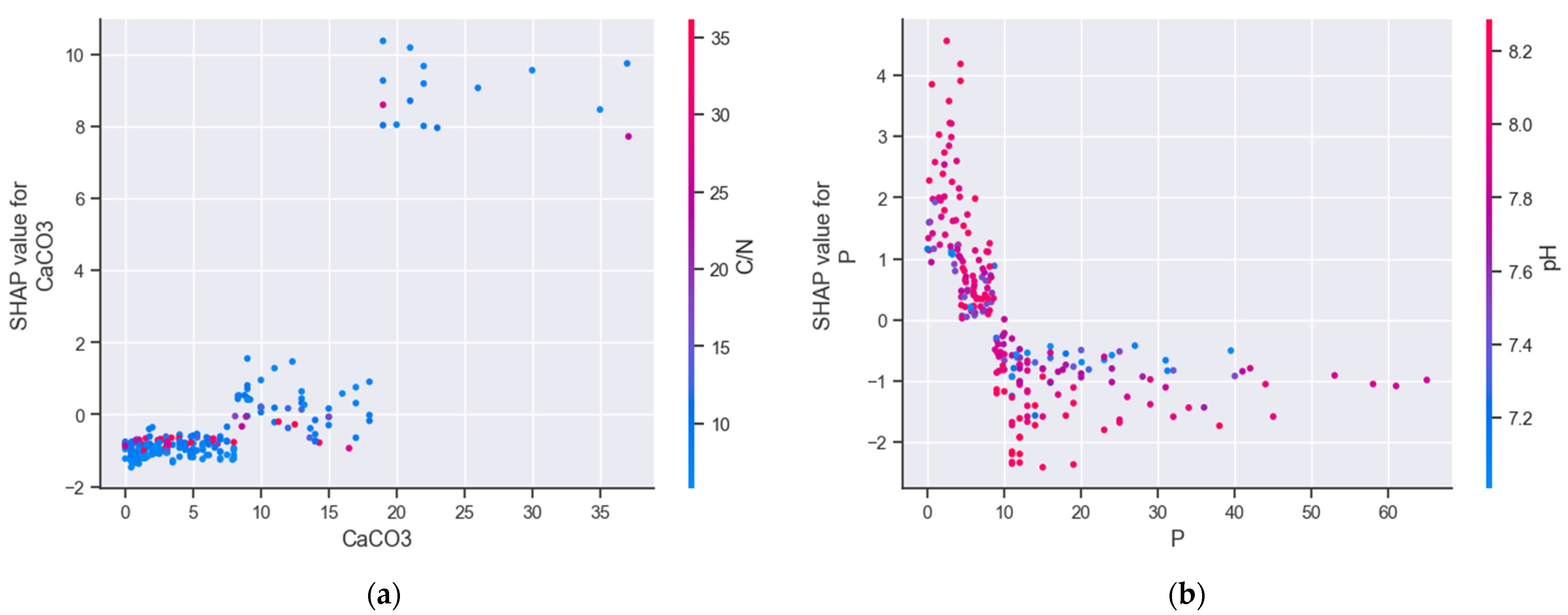
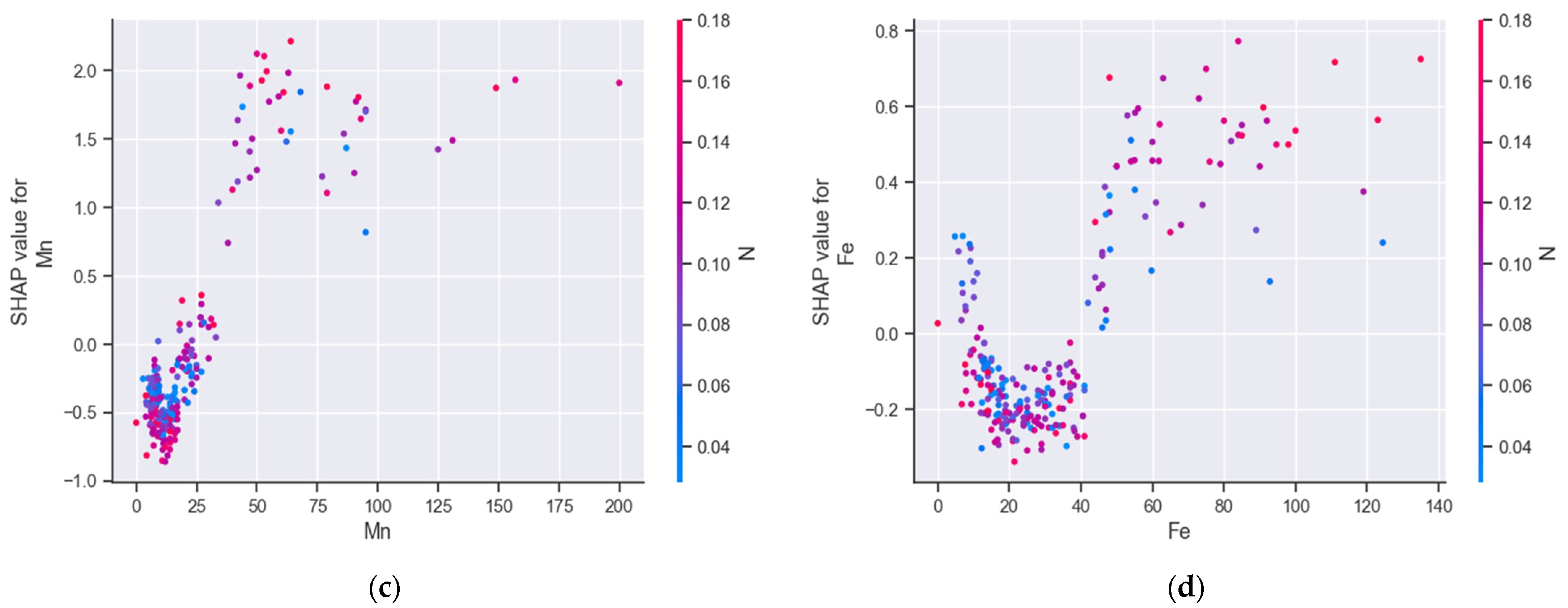
3.2. Machine Learning and SHAP Analysis

A prediction model was developed using a LightGBM regressor, where the target variable was the deposit depth and the input variables were the soil analysis data. The prediction model was trained to identify the relative importance of each variable on the deposit depth. The MAE of the model was equal to 5.37 cm of the deposit depth. MAE is a metric that is used to evaluate the performance of regression models. It measures the average magnitude of the errors in a set (test) of predictions. It is calculated as the average of the absolute differences between the predicted values and the actual values. The feature importance plot for the LightGBM model is presented in Figure 8. CaCO3, P, and Mn were found to be the most important features for the LightGBM model. This plot was used to understand how each feature influenced the prediction of the LightGBM model. The feature importance is listed in the y-axis, and it is sorted so that the most influential features are at the top and the least important at the bottom. The position of the point on the x-axis also indicates whether the effect of that feature value increases or decreases the prediction. Furthermore, the color of the points indicates the value of the feature for that observation, with a red color representing high value and a blue color low value. The density of the points indicates how much variation exists in the impact of a feature on the output. Thus, a SHAP feature importance plot, also known as a SHAP summary plot, is particularly useful for complex models such as the LightGBM regressor, which captures nonlinear relationships [48].
The SHAP dependence plots revealed that variables exhibiting highly significant correlations based on the Spearman test (p < 0.001), namely CaCO3, Fe, and Mn, demonstrated an upward trend as the deposit depth increased, as depicted in Figure 9a,c,d. However, it is noteworthy that the normalized SHAP values indicated a narrower range of increase for Fe (−0.2 to 0.8) in comparison to the other variables. Consequently, CaCO3 and Mn held higher positions in the feature importance plot (Figure 8), while Fe ranked low in the importance score. P, which has a connection with CaCO3, as demonstrated by the DirectLiNGAM algorithm (Figure 5), ranked second in the feature importance score (Figure 8) and decreased with increasing deposit depth. The primary interactions related to CaCO3, P, Mn, and Fe were the C to N ratio with CaCO3, pH with P, N with Mn, and N with Fe (Figure 9). It is worth noting that the C to N ratio exhibited a negative correlation with the soil deposit due to a significant increase in N within the soil deposit, as illustrated in Figure 8.
Finally, Figure 10 shows the relationship between CaCO3 and P for soils with sediment and without sediment. The kernel density plot shows that there was a trend of reduced P with increased values of CaCO3, which is known by the domain knowledge, and that mostly the soils with deposit had a higher than 10% CaCO3. CaCO3 and P were chosen for further exploration using the kernel density plot as they were ranked highest in the feature importance scores, as shown in Figure 8.

3.3. Crop Phosphorus Fertilizer Rate for Soils with Sediments

The Soil and Water Resources Institute’s Fertilization Advisory Software (FAS) was utilized to assess the P needs for corn in Thessaly, a crop that is commonly cultivated in the region. FAS integrates an equation for calculating the P fertilizer rate, which includes factors like soil texture, CaCO3 content, soil organic matter (SOM), available P, pH, and the specific P requirements of crops to achieve maximum yield [49]. As statistical differences of CaCO3 levels were observed for soil deposits above 10 cm (Figure 6a), the data were binned into two groups: soil deposits with less or more than 10 cm. This categorization was also driven by the observed variance in P needs for soils without deposits, ranging from completely depleted to highly available P, which is a normal finding in agricultural soils. The Shapiro test indicated non-normal variance in these groups. Thus, a Kruskal–Wallis test was carried out to test the difference between the two groups [50]. The analysis showed that 31.8% higher P fertilizer rates were needed for soils with greater than 10 cm sediments for avoiding yield reduction in corn (p = 0.001).

4. Discussion

This study conducted a causal discovery between the soil variables to trace the effect of sediment deposition on soil chemistry. The causal discovery algorithms presented in this study (DirectLiNGAM and RESIT) are capable of capturing the effect of soil deposit on soil chemistry as they are an evolution of the traditional causal algorithms employing the assumption on non-Gaussianity and non-linear causal discovery for DirectLiNGAM and RESIT, respectively. The results revealed a noteworthy effect of the soil deposit on CaCO3 content, which indirectly affected the P levels. The causal analysis, as shown in Figure 6, demonstrated that there was a downward trend of P concentration in relation to deposit depth, and the difference was significant for the soil that had deposits greater than 20 cm compared to the soils without deposits. The LightGBM algorithm also confirmed that there was a downward trend, but it was less conservative compared to the RESIT algorithm as it found that, for soils with sediments, it was unlikely to have a higher than 10 mg/kg P concentration (Figure 9). Interestingly, although P was identified as the second-most influential factor by the LightGBM algorithm, the Spearman correlation analysis did not mark it as significant in relation to the deposit depth variable. This highlights the non-linear association between the P levels and sediment presence.
Following nitrogen (N), P stands as a crucial nutrient essential for plant growth and overall productivity. Even though, normally, the soil contains P at levels around 2000 times higher than what is found in plants, its fixation in the form of aluminum/iron or calcium/magnesium phosphates renders it inaccessible for uptake by plants [24]. Consequently, plants frequently encounter the challenge of P deficiency in agricultural fields. Detecting this deficiency proved to not be an easy task, as the crops typically did not exhibit visual symptoms during the early stages [51]. Thus, there was no consistent chlorosis observed in the plants suffering from P deficiency. The shortage of P adversely affected plant growth, a consequence that was attributed to either a decrease in photosynthesis or an increase in energy investment. This limitation had a detrimental impact on both crop yield and quality. It was estimated that P deficiency leads to reduced crop yields on approximately 30–40% of the world’s arable land. In agricultural fields, the Phosphorus Use Efficiency (PUE) ranges around 15–20%, thereby indicating that a significant portion of the P applied to the soil remains inaccessible for plant uptake [52]. The reduced P availability due to sediment deposition in the flooded areas necessitates the use of increased P rates for the next growing season in Thessaly.
Corn was used as a model crop for running the FAS for all the soil samples taken from the study region. The analysis revealed that a 31.8% higher P fertilizer rate is necessary to avoid a yield reduction in the corn in Thessaly for the next growing season (Figure 11). The fertilizer types normally used in Thessaly for corn, according to the potassium levels at the various fields, are the following: (N-P-K) 21-7-10, 18-10-22, and 33-10-7. The rate at broadcasting for these fertilizers was about 600 kg/ha. Thus, the P rate was 42 or 60 kg/ha, according to the fertilizer type used, which was quite lower compared to the average 112 kg of P per ha suggested by FAS for soils without sediments. This necessitates extra care for applying higher rates for soils with sediments compared to those normally used in the Thessaly area.
Correlation analysis was not sufficient to explain the causality between the soil deposit and changes in nutrient availability in the soil. Despite that, a high Spearman correlation was observed between the soil deposit and Fe (there were some high Fe values in soils with deposit as shown in the Fe histogram of Figure 4), the causal analysis elucidated that the Fe concentration in the soil was not affected by the soil deposit. This result was also confirmed by the LightGBM algorithm, which classified Fe as low in the feature importance score (Figure 8) in explaining soil deposit variability. The directed acyclic graph (DAG) in Figure 5 shows that the effect of CaCO3 was negative on the Fe concentration in soil, which is known by the domain knowledge, as the formation of calcium–iron–phosphate compounds in the presence of CaCO3 can reduce the availability of the iron in the soil [53]. Thus, although there were some extreme Fe concentrations in the soil deposits, the presence of increased CaCO3 in the sediments resulted in the mitigation of iron in the soil, a trend which is also shown in Figure 6, as non-statistical differences were observed across the various deposit depths. This confirmed that the existence of correlation between variables was a necessary, but not sufficient, condition for causality [16].
The Mn concentration, though, presented an upward trend with an increase in deposit depth, which was confirmed by both the causal analysis and the LightGBM algorithm. However, even these increased levels of Mn, i.e., 45 mg/kg of soil (for the upward limit of the confidence interval at a 30 cm deposit depth, as shown in Figure 6) did not limit plant growth. This highlighted the effectiveness of bootstrapping with the RESIT algorithm, which enabled the construction of confidence intervals at the various levels of deposit depth. This also underscored the potential risks associated with the lack of interpretation for black box models, such as neural networks, a point that was further illustrated by Prendin et al. [11] However, the construction of confidence intervals for the estimated causal effects using bootstrapping allowed for an assessment of the causal effects on the soil properties. This was because the confidence intervals showed that the P decrease caused by the deposit could be limiting plant growth, while a Mn increase was not found to be toxic for plants. To further elucidate the effect of deposit on P and Mn availability, an ML algorithm (LightGBM) was used along with SHAP analysis. SHAP can offer an explanation on how much each feature relates to the target variable, i.e., deposit depth; thus, for the scope of this study, the ML procedure along with SHAP worked as a robustness check for the causal inference model. Finding consistent results across the ML and causal inference methods enhanced the credibility of the causal model. The use of causal machine learning along with the ML methods proved instrumental in transcending traditional correlation-based analyses, thus allowing us to pinpoint the direct and indirect effects of sediment deposition on soil chemistry. This approach provides a robust framework for developing adaptive agricultural practices in response to extreme weather events, which are becoming increasingly frequent due to climate change.
We found that some causal links between variables were controversial to domain knowledge. For example, CaCO3 affects P availability, but this does not apply vice versa. This observation might have likely stemmed from the limited size of the dataset. Nonetheless, the dataset size was inevitably small considering the extensive effort required to collect these samples from the flooded region and to identify areas with sediments, especially given the narrow timeframe available for collecting samples before the growers incorporated the sediments in the soil.
Other causal links identified by the DirectLiNGAM algorithm included the effect of deposit depth on sand and the ratio of organic carbon to total nitrogen (C/N). As the feature importance plot shows, the negative effect of the deposit depth on carbon to the total N ratio was mostly because of the increase in the total N content in the sediments (which was probably due to the transfer of floating organic matter together with the sediment). Thus, N availability will possibly be increased in the soils that have sediments, and N will not be limited for the next cropping season provided that the growers continue to apply the suggested rates of N fertilizers. Potassium availability was not affected by the sediment as potassium ranked last in the feature importance score (Figure 8).
In addition to soil chemistry, it is crucial for farmers to manage the physical properties of soils that are affected by sediment deposition. The presence of fine, silty particles with small pores can lead to waterlogging as these particles absorb water without allowing it to drain efficiently. This could result in a difficulty in root function and restrictions in the aeration of the soil beneath. To mitigate these issues and ensure optimal crop production, it is essential for the growers to incorporate these sediments thoroughly with the existing soil, thus ensuring a homogeneous mixture that maintains the soil’s physical properties.
Data on the soil’s biological activity relevant to the current study are not available. Nonetheless, a study by Shah et al. [54] has shown that, in scenarios where flooding is temporary (such in the Thessaly plain), microbial activity tends to recover swiftly. More specifically, according to their findings, microbiota in the soil can recover within three weeks after flooding.

5. Conclusions

The present study unveiled the significant impact of sediment deposition, a consequence of the unprecedented flood event that occurred due to Storm ‘Daniel’, on the soil chemical properties in the Thessaly region of Greece. Through soil sampling, chemical analysis, and the innovative application of causal machine learning algorithms, we elucidated the causal relationships between sediment deposition depth and CaCO3, available P, and Mn. Our findings reveal a significant effect of sediment depth on these crucial soil parameters, highlighting the necessity for tailored soil management strategies to counteract the effects of the deposit on agricultural productivity.
Our analysis indicates that corn crops in areas affected by sediment deposition exceeding 10 cm require a significant adjustment in P fertilization rates to avert potential yield declines. This insight is crucial for farmers and agricultural advisors in the region, as it provides a data-driven basis for fertilization decisions after the flooding event.
Finally, this study underscores the critical role of advanced machine learning techniques in environmental and agricultural sciences, thereby offering a paradigm for future research in the face of escalating climate variability.

Author Contributions

Conceptualization, M.I., A.T., E.E., C.N., D.V. and P.T.; methodology, M.I.; software, M.I.; validation, M.I.; formal analysis, M.I.; investigation, M.I., A.T., E.E., C.N., D.V. and P.T.; resources, M.T., A.T., E.E., C.N. and D.V.; data curation, M.I., V.A. and A.T.; writing—original draft preparation, M.I.; writing—review and editing, M.I., V.A., G.A., I.M. and C.K.; visualization, M.I., A.T. and P.T.; supervision, M.I.; project administration, D.V. and G.A.; funding acquisition, D.V. All authors have read and agreed to the published version of the manuscript.

Funding

This research received no external funding.

Institutional Review Board Statement

Not applicable.

Data Availability Statement

The data can be made available by contacting the corresponding authors.

Conflicts of Interest

The authors declare no conflicts of interest.

References

  1. European Academies Science Advisory Council. Extreme Weather Events in Europe Preparing for Climate Change Adaptation: An Update on EASAC’s 2013 Study. Available online: https://easac.eu/publications/details/extreme-weather-events-in-europe (accessed on 15 January 2024).
  2. Furtak, K.; Wolińska, A. The Impact of Extreme Weather Events as a Consequence of Climate Change on the Soil Moisture and on the Quality of the Soil Environment and Agriculture—A Review. Catena 2023, 231, 107378. [Google Scholar] [CrossRef]
  3. Loeb, R.; Lamers, L.P.M.; Roelofs, J.G.M. Effects of Winter versus Summer Flooding and Subsequent Desiccation on Soil Chemistry in a Riverine Hay Meadow. Geoderma 2008, 145, 84–90. [Google Scholar] [CrossRef]
  4. Christensen, J.H.; Christensen, O.B. Severe Summertime Flooding in Europe. Nature 2003, 421, 805–806. [Google Scholar] [CrossRef] [PubMed]
  5. Khatibi, E.; Abbasian, M.; Azimi, I.; Labbaf, S.; Feli, M.; Borelli, J.; Dutt, N.; Rahmani, A.M. Impact of COVID-19 Pandemic on Sleep Including HRV and Physical Activity as Mediators: A Causal ML Approach. In Proceedings of the 2023 IEEE 19th International Conference on Body Sensor Networks (BSN), Cambridge, MA, USA, 9–11 October 2023; pp. 1–4. [Google Scholar]
  6. Sanchez, P.; Voisey, J.P.; Xia, T.; Watson, H.I.; O’Neil, A.Q.; Tsaftaris, S.A. Causal Machine Learning for Healthcare and Precision Medicine. R. Soc. Open Sci. 2022, 9, 220638. [Google Scholar] [CrossRef]
  7. Karydas, C.; Iatrou, M.; Kouretas, D.; Patouna, A.; Iatrou, G.; Lazos, N.; Gewehr, S.; Tseni, X.; Tekos, F.; Zartaloudis, Z.; et al. Prediction of Antioxidant Activity of Cherry Fruits from UAS Multispectral Imagery Using Machine Learning. Antioxidants 2020, 9, 156. [Google Scholar] [CrossRef] [PubMed]
  8. Iatrou, M.; Karydas, C.; Iatrou, G.; Pitsiorlas, I.; Aschonitis, V.; Raptis, I.; Mpetas, S.; Kravvas, K.; Mourelatos, S. Topdressing Nitrogen Demand Prediction in Rice Crop Using Machine Learning Systems. Agriculture 2021, 11, 312. [Google Scholar] [CrossRef]
  9. Fehr, J.; Piccininni, M.; Kurth, T.; Konigorski, S. Assessing the Transportability of Clinical Prediction Models for Cognitive Impairment Using Causal Models. BMC Med. Res. Methodol. 2023, 23, 187. [Google Scholar] [CrossRef] [PubMed]
  10. Shimizu, S.; Inazumi, T.; Kawahara, Y.; Washio, T.; Hoyer Patrikhoyer, P.O.; Bollen, K.; Sogawa, Y.; Hyvärinen, A.; Hoyer, P.O.; Bollen Shimizu, K. DirectLiNGAM: A Direct Method for Learning a Linear Non-Gaussian Structural Equation Model Yasuhiro Sogawa Aapo Hyvärinen. J. Mach. Learn. Res. 2011, 12, 1225–1248. [Google Scholar]
  11. Prendin, F.; Pavan, J.; Cappon, G.; Del Favero, S.; Sparacino, G.; Facchinetti, A. The Importance of Interpreting Machine Learning Models for Blood Glucose Prediction in Diabetes: An Analysis Using SHAP. Sci. Rep. 2023, 13, 16865. [Google Scholar] [CrossRef] [PubMed]
  12. Lundberg, S.M.; Lee, S.-I. A Unified Approach to Interpreting Model Predictions. arXiv 2017, arXiv:1705.07874. [Google Scholar]
  13. Wojtuch, A.; Jankowski, R.; Podlewska, S. How Can SHAP Values Help to Shape Metabolic Stability of Chemical Compounds? J. Cheminform. 2021, 13, 74. [Google Scholar] [CrossRef] [PubMed]
  14. Lloyd, S. N-Person Games. Def. Tech. Inf. Cent. 1952, 295–314. [Google Scholar] [CrossRef]
  15. Gramegna, A.; Giudici, P. SHAP and LIME: An Evaluation of Discriminative Power in Credit Risk. Front. Artif. Intell. 2021, 4, 752558. [Google Scholar] [CrossRef] [PubMed]
  16. Niyogi, D.; Kishtawal, C.; Tripathi, S.; Govindaraju, R.S. Observational Evidence That Agricultural Intensification and Land Use Change May Be Reducing the Indian Summer Monsoon Rainfall. Water Resour. Res. 2010, 46, 1–17. [Google Scholar] [CrossRef]
  17. Copernicus Emergency Management Service Directorate Space, Security and Migration, European Commission Joint Research Centre (EC JRC). Available online: https://emergency.copernicus.eu/ (accessed on 25 November 2023).
  18. Miller, J.; Curtin, D. Electrical Conductivity and Soluble Ions. 2007. Available online: https://www.researchgate.net/publication/288518660_Electrical_Conductivity_and_Soluble_Ions (accessed on 19 December 2023).
  19. Gavlak, R.G.; Horneck, D.A.; Miller, R.O. Plant, Soil, and Water Reference Methods for the Western Region; Western Rural Development Center: Logan, UT, USA, 1994. [Google Scholar]
  20. Pearson, D. The Chemical Analysis of Foods, 7th ed.; Churchill Livingstone: London, UK, 1976. [Google Scholar]
  21. Walkley, A.; Black, I.A. An examination of the degtjareff method for determining soil organic matter, and a proposed modification of the chromic acid titration method. Soil Sci. 1934, 37, 29–38. [Google Scholar] [CrossRef]
  22. Van Reeuwijk, L.P. Procedures for Soil Analysis. 2002. Available online: https://www.isric.org/sites/default/files/ISRIC_TechPap09.pdf (accessed on 23 November 2023).
  23. Bouyoucos, G.J. Hydrometer Method Improved for Making Particle Size Analyses of Soils. Agron. J. 1962, 54, 464–465. [Google Scholar] [CrossRef]
  24. Iatrou, M.; Papadopoulos, A.; Papadopoulos, F.; Dichala, O.; Psoma, P.; Bountla, A. Determination of Soil Available Phosphorus Using the Olsen and Mehlich 3 Methods for Greek Soils Having Variable Amounts of Calcium Carbonate. Commun. Soil Sci. Plant Anal. 2014, 45, 2207–2214. [Google Scholar] [CrossRef]
  25. Knudsen, D.; Peterson, G.A.; Pratt, P.F. Lithium, Sodium, and Potassium. In Methods of Soil Analysis; Agronomy Monographs; Wiley: Hoboken, NJ, USA, 1983; pp. 225–246. ISBN 9780891189770. [Google Scholar]
  26. Iatrou, M.; Papadopoulos, A.; Papadopoulos, F.; Dichala, O.; Psoma, P.; Bountla, A. Determination of Soil-Available Micronutrients Using the DTPA and Mehlich 3 Methods for Greek Soils Having Variable Amounts of Calcium Carbonate. Commun. Soil Sci. Plant Anal. 2015, 46, 1905–1912. [Google Scholar] [CrossRef]
  27. Breiman, L. Random Forests. Mach. Learn. 2001, 45, 5–32. [Google Scholar] [CrossRef]
  28. Howard, J.; Gugger, S. Deep Learning for Coders with Fastai and PyTorch; O’Reilly Media: Sebastopol, ON, Canada, 2020. [Google Scholar]
  29. Howard, J.; Gugger, S. Fastai: A Layered API for Deep Learning. arXiv 2020, arXiv:2002.04688. [Google Scholar] [CrossRef]
  30. Ke, G.; Meng, Q.; Finley, T.; Wang, T.; Chen, W.; Ma, W.; Ye, Q.; Liu, T.-Y. LightGBM: A Highly Efficient Gradient Boosting Decision Tree. In Proceedings of the Advances in Neural Information Processing Systems; Guyon, I., Von Luxburg, U., Bengio, S., Wallach, H., Fergus, R., Vishwanathan, S., Garnett, R., Eds.; Curran Associates, Inc.: Red Hook, NY, USA, 2017; Volume 30. [Google Scholar]
  31. Iatrou, M.; Karydas, C.; Tseni, X.; Mourelatos, S. Representation Learning with a Variational Autoencoder for Predicting Nitrogen Requirement in Rice. Remote Sens. 2022, 14, 5978. [Google Scholar] [CrossRef]
  32. Chen, T.; Guestrin, C. XGBoost: A Scalable Tree Boosting System. In Proceedings of the 22nd ACM SIGKDD International Conference on Knowledge Discovery and Data Mining, San Francisco, CA, USA, 13–17 August 2016; ACM: New York, NY, USA, 2016; pp. 785–794. [Google Scholar]
  33. Akiba, T.; Sano, S.; Yanase, T.; Ohta, T.; Koyama, M. Optuna: A Next-Generation Hyperparameter Optimization Framework. arXiv 2019, arXiv:1907.10902. [Google Scholar]
  34. Madhushani, C.; Dananjaya, K.; Ekanayake, I.U.; Meddage, D.P.P.; Kantamaneni, K.; Rathnayake, U. Modeling Streamflow in Non-Gauged Watersheds with Sparse Data Considering Physiographic, Dynamic Climate, and Anthropogenic Factors Using Explainable Soft Computing Techniques. J. Hydrol. 2024, 631, 130846. [Google Scholar] [CrossRef]
  35. Joseph, A. Shapley Regressions: A Framework for Statistical Inference on Machine Learning Models, 4th ed.; Bank of England and King’s College London: London, UK, 2019. [Google Scholar]
  36. Howard, R.; Kunze, L. Evaluating Temporal Observation-Based Causal Discovery Techniques Applied to Road Driver Behaviour. arXiv 2023, arXiv:2302.00064. [Google Scholar]
  37. Pearl, J. Causal Diagrams for Empirical Research. Biometrika 1995, 82, 669–688. [Google Scholar] [CrossRef]
  38. Hyvärinen, A.; Smith, S.M.; Spirtes, P. Pairwise Likelihood Ratios for Estimation of Non-Gaussian Structural Equation Models. J. Mach. Learn. Res. 2013, 14, 111–152. [Google Scholar] [PubMed]
  39. Hoyer, P.O.; Janzing, D.; Mooij, J.; Peters, J.; Schölkopf, B. Nonlinear Causal Discovery with Additive Noise Models. In Proceedings of the 21st International Conference on Neural Information Processing Systems, Kuching, Malaysia, 3–6 November 2014; Curran Associates Inc.: Red Hook, NY, USA, 2014; pp. 689–696. [Google Scholar]
  40. Peters, J.; Mooij, J.M.; Janzing, D.; Schölkopf, B. Causal Discovery with Continuous Additive Noise Models. arXiv 2014, arXiv:1309.6779. [Google Scholar]
  41. Strobl, E.V.; Lasko, T.A. Identifying Patient-Specific Root Causes with the Heteroscedastic Noise Model. J. Comput. Sci. 2023, 72, 102099. [Google Scholar] [CrossRef]
  42. Komatsu, Y.; Shimizu, S.; Shimodaira, H. Assessing Statistical Reliability of LiNGAM via Multiscale Bootstrap. In Proceedings of the 20th International Conference on Artificial Neural Networks: Part III, Thessaloniki Greece, 15–18 September 2010; Springer: Berlin/Heidelberg, Germany, 2010; pp. 309–314. [Google Scholar]
  43. Brownlee, J. Deep Learning with Python. Develop Deep Learning Models on Theano and Tensorf Flow Using Keras. Machine Learning Mastery. 2018. Available online: https://bayanbox.ir/view/269467307605579794/deep-learning-with-python.pdf (accessed on 20 December 2023).
  44. Brownlee, J. Better Deep Learning. Train Faster, Reduce Overfitting, and Make Better Predictions; Machine Learning Mastery: San Juan, Puerto Rico, 2019. [Google Scholar]
  45. Van Rossum, G.; Drake, F.L. Python Tutorial. History 2010, 42, 270–272. [Google Scholar] [CrossRef]
  46. Hunter, J.D. Matplotlib: A 2D Graphics Environment. Comput. Sci. Eng. 2007, 9, 90–95. [Google Scholar] [CrossRef]
  47. Waskom, M.; Botvinnik, O.; O’Kane, D.; Hobson, P.; Lukauskas, S.; Gemperline, D.C.; Augspurger, T.; Halchenko, Y.; Cole, J.B.; Warmenhoven, J.; et al. Mwaskom/Seaborn: V0.8.1 (September 2017). 2017. Available online: https://zenodo.org/records/883859 (accessed on 14 November 2023). [CrossRef]
  48. Cakiroglu, C.; Demir, S.; Hakan Ozdemir, M.; Latif Aylak, B.; Sariisik, G.; Abualigah, L. Data-Driven Interpretable Ensemble Learning Methods for the Prediction of Wind Turbine Power Incorporating SHAP Analysis. Expert Syst. Appl. 2024, 237, 121464. [Google Scholar] [CrossRef]
  49. Papadopoulos, A.; Papadopoulos, F.; Tziachris, P.; Metaxa, I.; Iatrou, M. Site Specific Management with the Use of a Digitized Soil Map for the Regional Unit of Kastoria. Ecosyst. Nat. Resour. Manag. 2014, 16, 59–67. [Google Scholar]
  50. Kruskal, W.H.; Wallis, W.A. Use of Ranks in One-Criterion Variance Analysis. J. Am. Stat. Assoc. 1952, 47, 583–621. [Google Scholar] [CrossRef]
  51. Malhotra, H.; Vandana; Sharma, S.; Pandey, R. Phosphorus Nutrition: Plant Growth in Response to Deficiency and Excess. In Plant Nutrients and Abiotic Stress Tolerance; Hasanuzzaman, M., Fujita, M., Oku, H., Nahar, K., Hawrylak-Nowak, B., Eds.; Springer: Singapore, 2018; pp. 171–190. ISBN 978-981-10-9044-8. [Google Scholar]
  52. Biswas Chowdhury, R.; Zhang, X. Phosphorus Use Efficiency in Agricultural Systems: A Comprehensive Assessment through the Review of National Scale Substance Flow Analyses. Ecol. Indic. 2021, 121, 107172. [Google Scholar] [CrossRef]
  53. Loeppert, R.H. Reactions of Iron and Carbonates in Calcareous Soils. J. Plant Nutr. 1986, 9, 195–214. [Google Scholar] [CrossRef]
  54. Shah, A.; Shah, S.; Shah, V. Impact of Flooding on the Soil Microbiota. Environ. Chall. 2021, 4, 100134. [Google Scholar] [CrossRef]
Figure 1. (a) Map of the area before flooding. (b) Flooded areas on 7 September 2023.
Agriculture 14 00549 g001
Figure 2. Photos showing the extent of sediment accumulation following the recession of floodwaters.
Agriculture 14 00549 g002
Figure 3. Overview of the processes used for defining and quantifying the effect of sediment on the soil properties.
Agriculture 14 00549 g003
Figure 4. The probability histograms show the distribution of Cu, Fe, and Mn.
Agriculture 14 00549 g004
Figure 5. Directed acyclic graph of the soil variables. The directed arrows indicate the causal relationships between variables. The direction of the arrow captures the direction of causality.
Agriculture 14 00549 g005
Figure 6. Effect of the deposit depth using the RESIT method on (a) CaCO3; (b) P; (c) Mn; and (d) Fe. The boxplots show the distribution of the causal effect of the deposit depth and outliers are also shown at the 95% level as “°”.
Agriculture 14 00549 g006aAgriculture 14 00549 g006b
Figure 7. Relationships of the deposit depth with CaCO3, P, and Mn. These equations indicated that the relationships followed a quadratic trend.
Agriculture 14 00549 g007
Figure 8. The results of the feature evaluation using SHAP for the feature importance of the LightGBM model.
Agriculture 14 00549 g008
Figure 9. SHAP dependence plots showing the interactions of (a) CaCO3; (b) P; (c) Mn; and (d) Fe. The SHAP value indicates how much the value of a soil variable changes the prediction of the deposit depth.
Agriculture 14 00549 g009aAgriculture 14 00549 g009b
Figure 10. Kernel density plot showing the relationship between CaCO3 and P for soils with deposit (red color) and without deposit (blue color).
Agriculture 14 00549 g010
Figure 11. The corn P fertilizer rate for deposit depths that were less or more than 10 cm. Error bars display the standard error of means (s.e.m.).
Agriculture 14 00549 g011
Table 1. Input variables of the LightGBM regressor.
Soil VariablesDefinitionMeanStd *
ClayWeight percentage of clay26.56%14.00
SandWeight percentage of sand38.99%13.09
SiltWeight percentage of silt34.41%10.64
pHSoil pH in soil to water ratio 1:17.820.43
ECElectrical conductivity in soil to water ratio 1:1480.14 μS/cm318.82
CaCO3Calcium carbonate content6.8%7.28
SOMSoil organic matter content1.71%0.63
NTotal Kjeldahl soil nitrogen0.1%0.05
C/NRatio of organic carbon to nitrogen12.9410.72
POlsen extractable phosphorus11.78 mg/kg10.74
KAmmonium acetate extractable potassium0.6 cmol/g0.37
CuDTPA extractable copper2.83 mg/kg2.00
FeDTPA extractable iron31.19 mg/kg23.64
MnDTPA extractable manganese23.08 mg/kg27.02
* Std = standard deviation. Number of observations (n) = 296.
Disclaimer/Publisher’s Note: The statements, opinions and data contained in all publications are solely those of the individual author(s) and contributor(s) and not of MDPI and/or the editor(s). MDPI and/or the editor(s) disclaim responsibility for any injury to people or property resulting from any ideas, methods, instructions or products referred to in the content.

