
A Combined Paddy Field Inter-Row Weeding Wheel Based on Display Dynamics Simulation Increasing Weed Mortality

 ,
, 


Abstract
1. Introduction
2. Materials and Methods
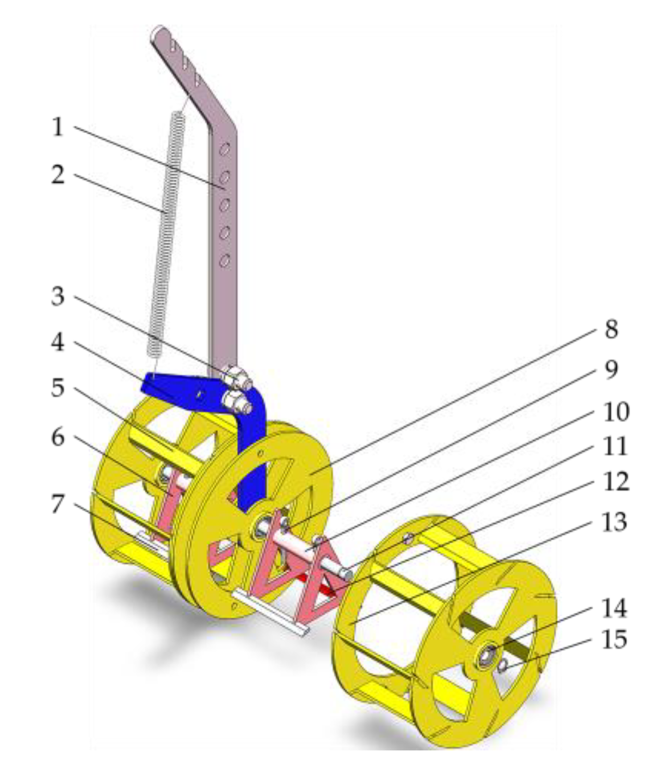
2.1. Overall Structure and Working Principle of the Combination Rice Field Inter-Row Weeding Wheel
2.2. Device Design
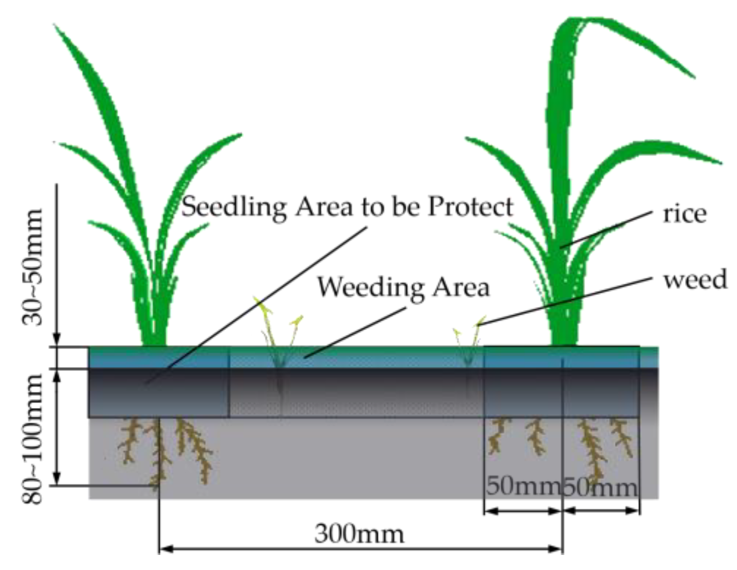
2.2.1. Rice Planting and Weed Control Agricultural Requirements in Northeastern China
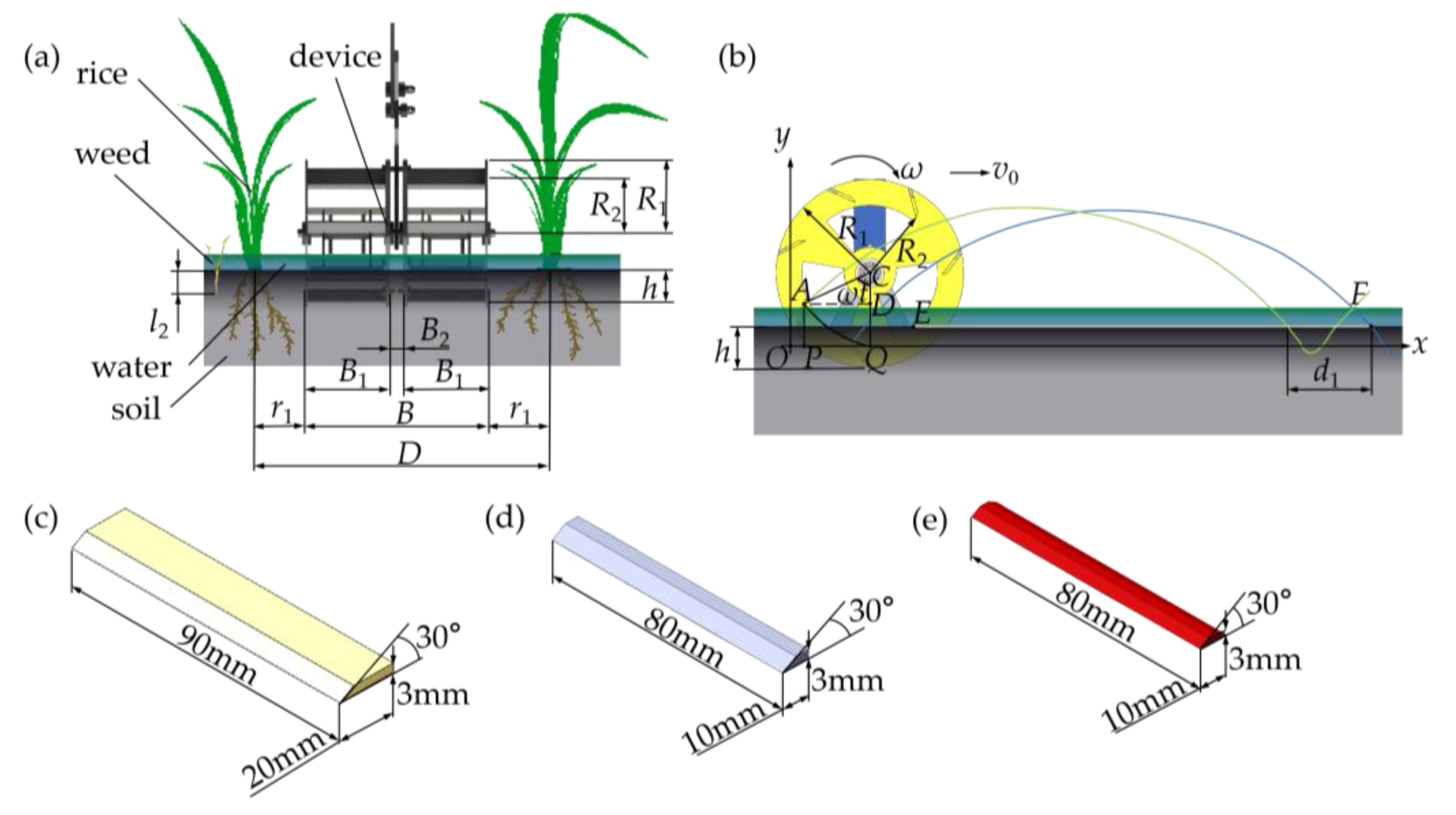
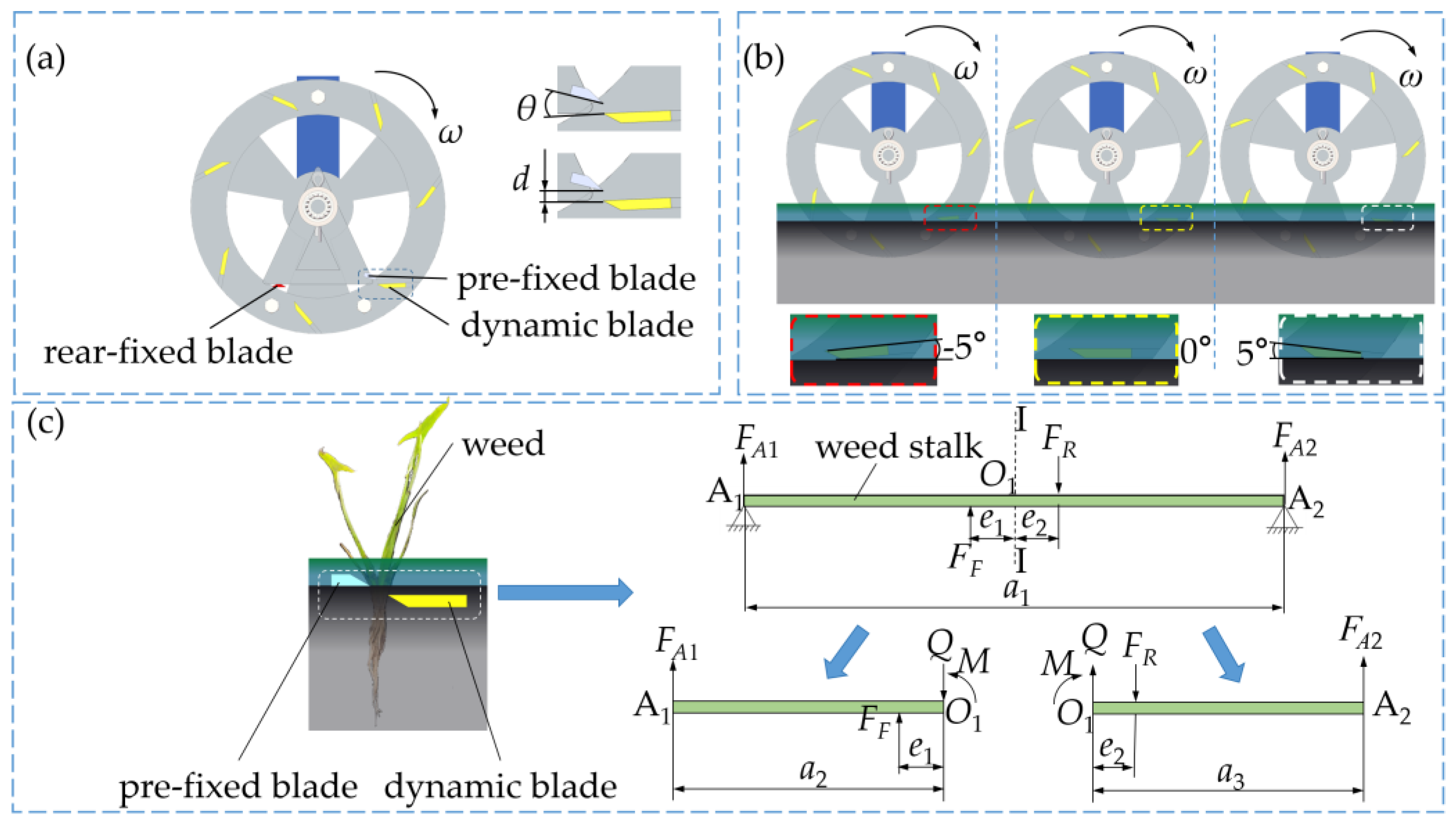
2.2.2. Designing Device Structural and Operating Parameters
2.2.3. Pending Structural Parameters
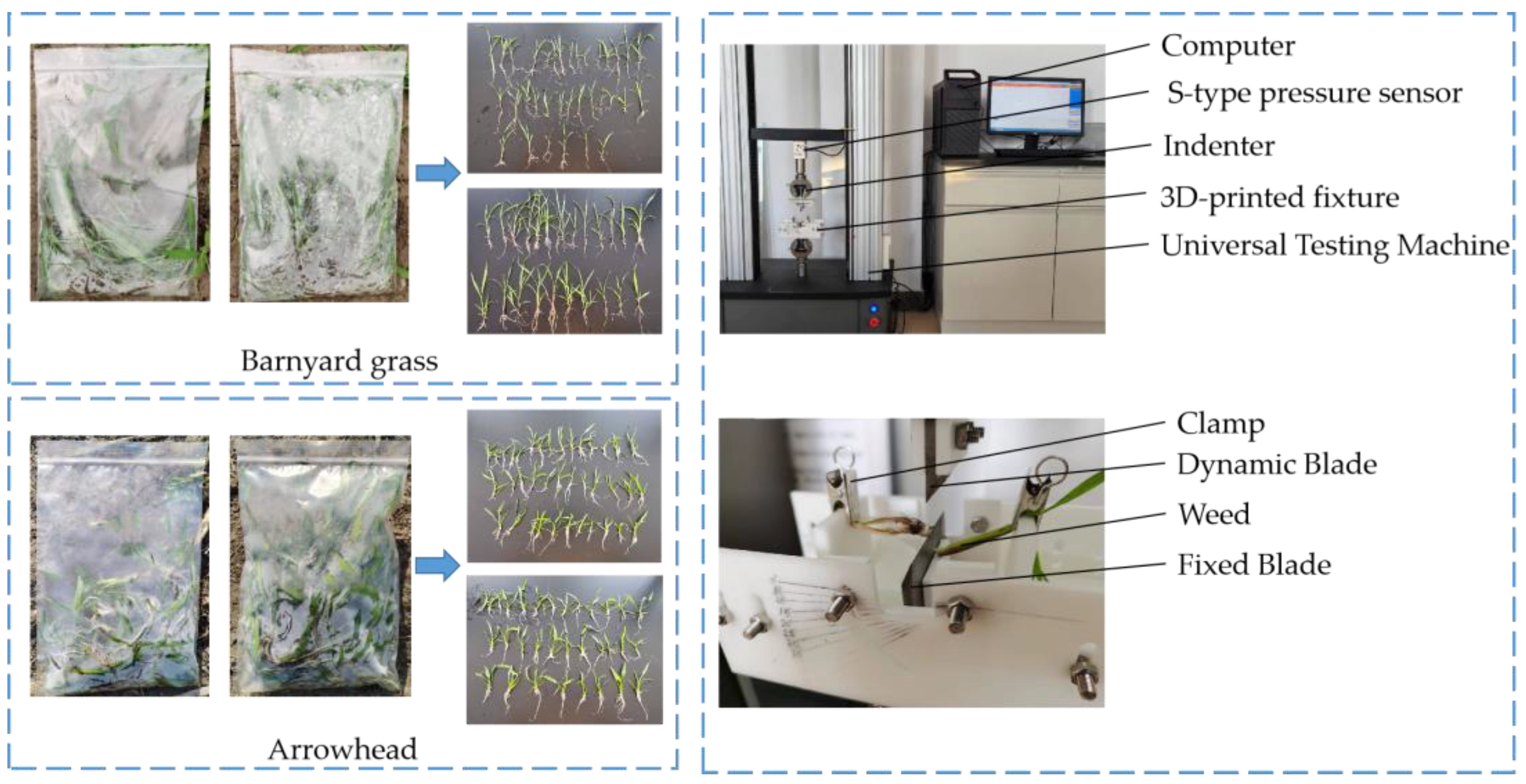
2.3. Paddy Field Weed Cutting Mechanical Properties Experiment
2.3.1. Experimental Materials and Equipment
2.3.2. Experimental Method
2.4. Structural Parameter Optimization Based on LS-DYNA
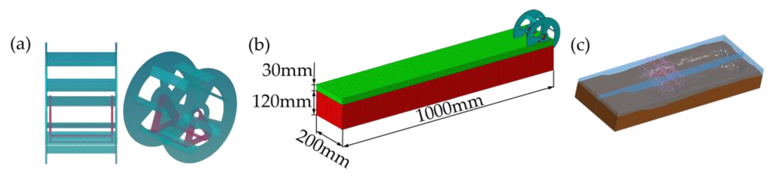
2.4.1. Establishment of the Weeding Wheel–Water–Soil Coupled Model
2.4.2. Experimental Method
2.4.3. Calculation Method for Experimental Metrics
- (1)
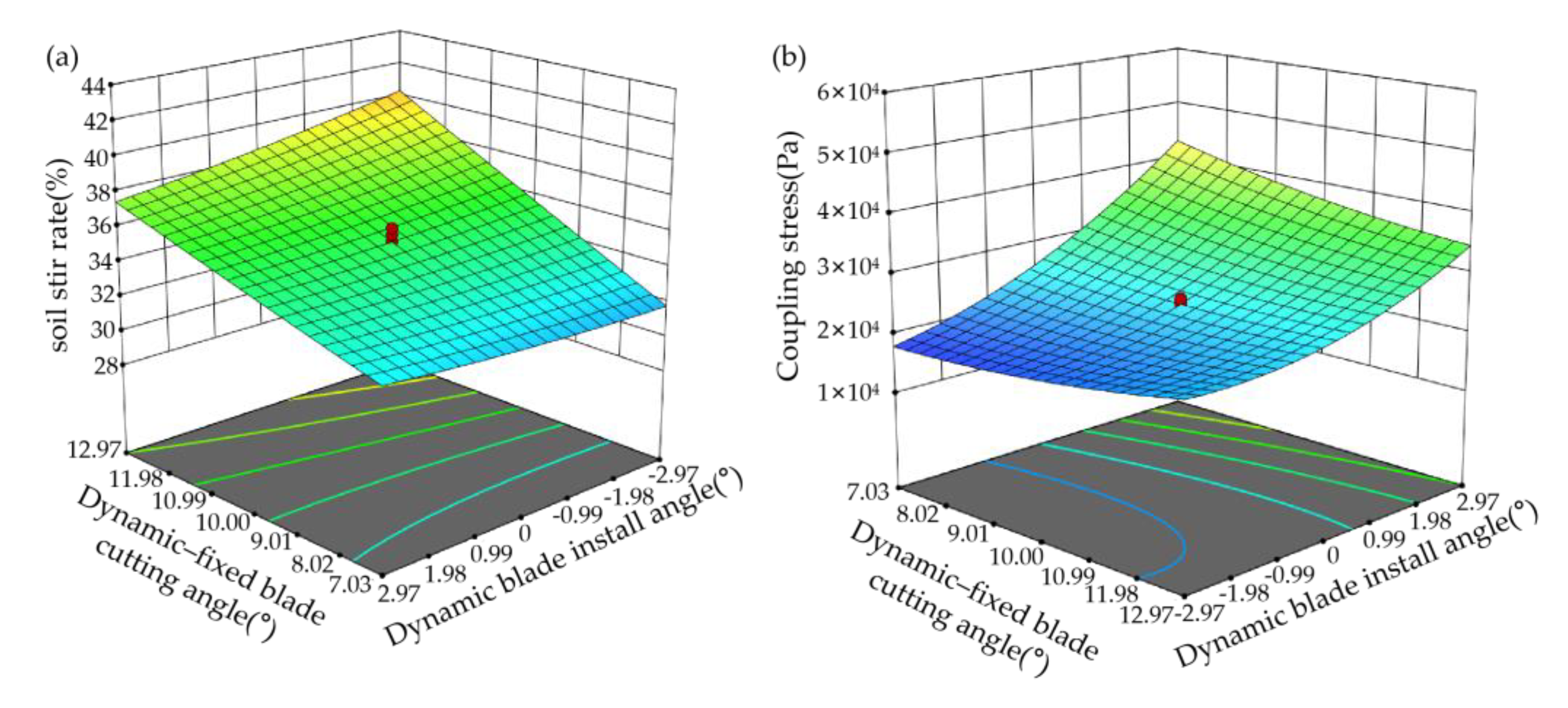
- Soil stir rate
- (2)
- Coupling stress
2.5. Field Experiment
2.5.1. Experimental Conditions
2.5.2. Experimental Method
2.5.3. Calculation of Experimental Metrics
3. Results and Discussion
3.1. Experimental Results
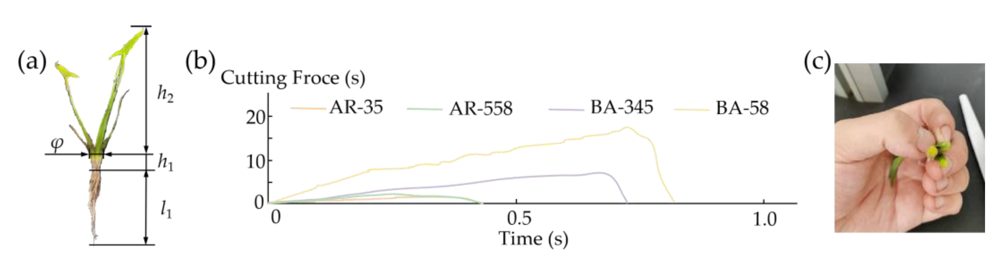
3.1.1. Results of Weed Cutting Mechanics Tests
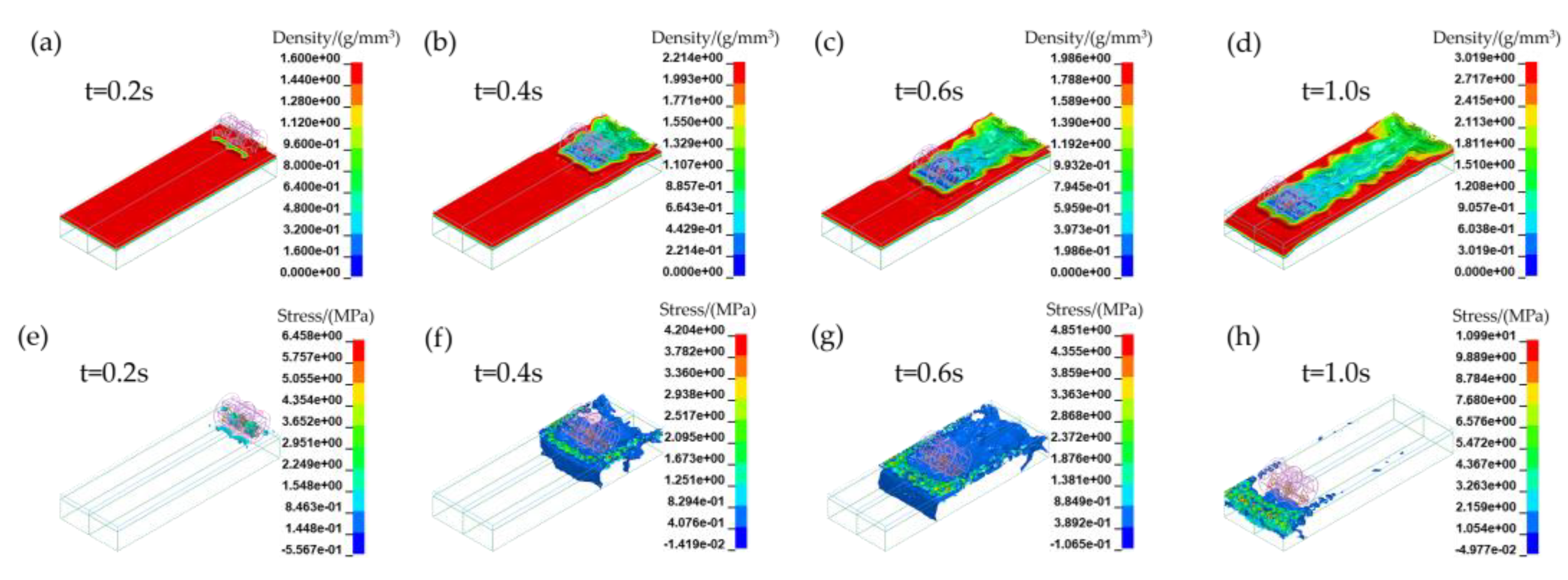
3.1.2. Results of Simulation Tests
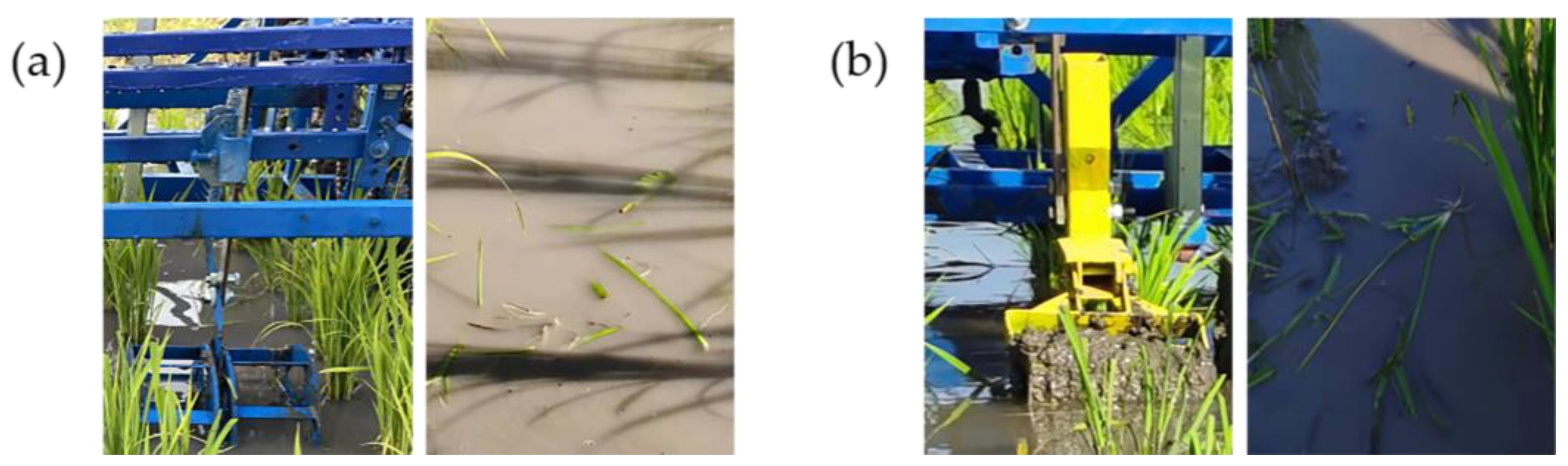
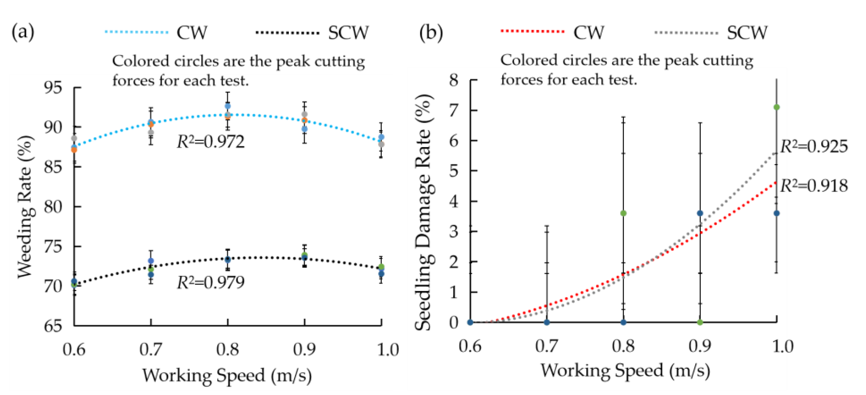
3.1.3. Field Experiment Results
3.2. Discussion
3.2.1. Discussion of Weed Cutting Mechanics Test Results
3.2.2. Discussion of Simulation Test Results
3.2.3. Discussion of Field Test Results
4. Conclusions
- (1)
- Theoretical analysis of the operational process of the designed combination weeding wheel led to the determination of certain parameters: h = 40 mm, B = 200 mm, R1 = 90 mm, R2 = 70 mm, Z = 7, and d1 = 63 mm.
- (2)
- A single factor test on the mechanical properties of weed cutting was carried out. The results show that d has a significant effect on the peak cutting force of BA-58, but no significant effect on the peak cutting force of BA-345, AR-35, and AR-558. Within the range of d from 0.6 to 1.4 mm, the peak cutting force on BA-58 reached its minimum. θ has a highly significant effect on the peak cutting force of BA-345, BA-58, and AR-35, and has a significant effect on the peak cutting force of AR-558. Within the range of θ from 5 to 15°, the peak cutting force on the above four weeds appeared to be the minimum.
- (3)
- A coupled simulation model of the weeding wheel–soil–water FSI was established using explicit dynamics simulation technology (LS-DYNA). A three-factor, five-level simulation test based on the central composite experimental design principle was conducted. The optimal structural parameters for the device were determined to be the following: d is 1.4 mm, θ is 10.95°, and α is −3.44°.
- (4)
- A comparative field experiment was conducted between the CW and SCW. The results revealed that the average weeding rate of the CW was 89.7%, and the seedling injury rate was 2.2%. The average weeding rate of the SCW was 72.3%, and the average seedling injury rate was 2.4%. The average weeding rate of the CW was significantly more outperforming than that of the SCW, and there was no significant difference in the average seedling injury rate between the CW and SCW.
Author Contributions
Funding
Institutional Review Board Statement
Data Availability Statement
Acknowledgments
Conflicts of Interest
References
- Birla, D.S.; Malik, K.; Sainger, M.; Chaudhary, D.; Jaiwal, R.; Jaiwal, P.K. Progress and Challenges in Improving the Nutritional Quality of Rice (Oryza sativa L.). Crit. Rev. Food Sci. Nutr. 2017, 57, 2455–2481. [Google Scholar] [CrossRef]
- Sen, S.; Chakraborty, R.; Kalita, P. Rice—Not Just a Staple Food: A Comprehensive Review on Its Phytochemicals and Therapeutic Potential. Trends Food Sci. Technol. 2020, 97, 265–285. [Google Scholar] [CrossRef]
- Young, S.L.; Anderson, J.V.; Baerson, S.R.; Bajsa-Hirschel, J.; Blumenthal, D.M.; Boyd, C.S.; Boyette, C.D.; Brennan, E.B.; Cantrell, C.L.; Chao, W.S.; et al. Agricultural Research Service Weed Science Research: Past, Present, and Future. Weed Sci. 2023, 71, 312–327. [Google Scholar] [CrossRef]
- Ragesh, K.T.; Jogdand, S.V.; Victor, V.M. Field Performance Evaluation of Power Weeder for Paddy Crop. Curr. Agric. Res. J. 2018, 6, 441–448. [Google Scholar] [CrossRef]
- Bennett, A.J.; Yadav, R.; Jha, P. Using Soybean Chaff Lining to Manage Waterhemp (Amaranthus tuberculatus) in a Soybean–Corn Rotation. Weed Sci. 2023, 71, 395–402. [Google Scholar] [CrossRef]
- Domingo, C.; San Segundo, B. Rice Thematic Special Issue: Beneficial Plant–Microbe Interactions in Rice. Rice 2023, 16, 50. [Google Scholar] [CrossRef] [PubMed]
- Hasanuzzaman, M.; Mohsin, S.M.; Bhuyan, M.H.M.B.; Bhuiyan, T.F.; Anee, T.I.; Masud, A.A.C.; Nahar, K. Phytotoxicity, Environmental and Health Hazards of Herbicides: Challenges and Ways Forward. In Agrochemicals Detection, Treatment and Remediation; Elsevier: Amsterdam, The Netherlands, 2020; pp. 55–99. [Google Scholar]
- Zeng, Z.; Martin, A.; Chen, Y.; Ma, X. Weeding Performance of a Spring-Tine Harrow as Affected by Timing and Operational Parameters. Weed Sci. 2021, 69, 247–256. [Google Scholar] [CrossRef]
- Shaner, D.L.; Beckie, H.J. The Future for Weed Control and Technology. Pest Manag. Sci. 2014, 70, 1329–1339. [Google Scholar] [CrossRef] [PubMed]
- Ranji, A.; Parashkoohi, M.G.; Zamani, D.M.; Ghahderijani, M. Evaluation of Agronomic, Technical, Economic, and Environmental Issues by Analytic Hierarchy Process for Rice Weeding Machine. Energy Rep. 2022, 8, 774–783. [Google Scholar] [CrossRef]
- Liu, C.; Yang, K.; Chen, Y.; Gong, H.; Feng, X.; Tang, Z.; Fu, D.; Qi, L. Benefits of Mechanical Weeding for Weed Control, Rice Growth Characteristics and Yield in Paddy Fields. Field Crops Res. 2023, 293, 108852. [Google Scholar] [CrossRef]
- Pareja, L.; Pérez-Parada, A.; Agüera, A.; Cesio, V.; Heinzen, H.; Fernández-Alba, A.R. Photolytic and Photocatalytic Degradation of Quinclorac in Ultrapure and Paddy Field Water: Identification of Transformation Products and Pathways. Chemosphere 2012, 87, 838–844. [Google Scholar] [CrossRef]
- Jones, E.A.L.; Austin, R.; Dunne, J.C.; Leon, R.G.; Everman, W.J. Discrimination between Protoporphyrinogen Oxidase–Inhibiting Herbicide-Resistant and Herbicide-Susceptible Redroot Pigweed (Amaranthus retroflexus) with Spectral Reflectance. Weed Sci. 2023, 71, 198–205. [Google Scholar] [CrossRef]
- Dayan, F.E.; Howell, J.; Marais, J.P.; Ferreira, D.; Koivunen, M. Manuka Oil, A Natural Herbicide with Preemergence Activity. Weed Sci. 2011, 59, 464–469. [Google Scholar] [CrossRef]
- Owen, M.D.K. Diverse Approaches to Herbicide-Resistant Weed Management. Weed Sci. 2016, 64, 570–584. [Google Scholar] [CrossRef]
- Richard, D.; Leimbrock-Rosch, L.; Keßler, S.; Stoll, E.; Zimmer, S. Soybean Yield Response to Different Mechanical Weed Control Methods in Organic Agriculture in Luxembourg. Eur. J. Agron. 2023, 147, 126842. [Google Scholar] [CrossRef]
- Cordill, C.; Grift, T.E. Design and Testing of an Intra-Row Mechanical Weeding Machine for Corn. Biosyst. Eng. 2011, 110, 247–252. [Google Scholar] [CrossRef]
- Gao, Y.; Zhu, Y.; Zhang, Y.; Zhang, Y.; Wang, Y.; Wang, Z.; Chen, H.; Zhang, Y.; Xiang, J. Physiological Characteristics of Root Regeneration in Rice Seedlings. Agronomy 2023, 13, 1772. [Google Scholar] [CrossRef]
- Qi, L.; Zhao, L.; Ma, X.; Cui, H.; Zheng, W.; Lu, Y. Design and Experiment of 3GY-1920 Wide-Swath Type Weeding-Cultivating Machine for Paddy. Trans. Chin. Soc. Agric. Eng. 2017, 33, 47–55. [Google Scholar] [CrossRef]
- Wang, J.; Gao, G.; Yan, D.; Wang, J.; Weng, W.; Chen, B. Design and Experiment of Electric Control Double Row Deep Fertilizing Weeder in Paddy Field. Trans. Chin. Soc. Agric. Mach. 2018, 49, 46–57. [Google Scholar]
- Wang, J.; Weng, W.; Ju, J.; Chen, X.; Wang, J.; Wang, H. Design and Experiment of Weeder between Rows in Rice Field Based on Remote Control Steering. Trans. Chin. Soc. Agric. Mach. 2021, 52, 97–105. [Google Scholar]
- Zhang, Y.; Tian, L.; Cao, C.; Zhu, C.; Qin, K.; Ge, J. Optimization and Validation of Blade Parameters for Inter-Row Weeding Wheel in Paddy Fields. Front. Plant Sci. 2022, 13, 1003471. [Google Scholar] [CrossRef]
- Kurstjens, D.A.G.; Kropff, M.J. The Impact of Uprooting and Soil-covering on the Effectiveness of Weed Harrowing. Weed Res. 2001, 41, 211–228. [Google Scholar] [CrossRef]
- Soleimani, N.; Kamandar, M.R.; Khoshnam, F.; Soleimani, A. Defining and Modelling Sesame Stalk Shear Behaviour in Harvesting by Reciprocating Cutting Blade. Biosyst. Eng. 2023, 229, 44–56. [Google Scholar] [CrossRef]
- Chattopadhyay, P.S.; Pandey, K.P. Effect of Knife and Operational Parameters on Energy Requirement in Flail Forage Harvesting. J. Agric. Eng. Res. 1999, 73, 3–12. [Google Scholar] [CrossRef]
- Allameh, A.; Reza Alizadeh, M. Specific Cutting Energy Variations under Different Rice Stem Cultivars and Blade Parameters. Idesia 2016, 34, 11–17. [Google Scholar] [CrossRef]
- Song, S.; Zhou, H.; Xu, L.; Jia, Z.; Hu, G. Cutting Mechanical Properties of Sisal Leaves under Rotary Impact Cutting. Ind. Crops Prod. 2022, 182, 114856. [Google Scholar] [CrossRef]
- Aydın, İ.; Arslan, S. Mechanical Properties of Cotton Shoots for Topping. Ind. Crops Prod. 2018, 112, 396–401. [Google Scholar] [CrossRef]
- Ramesh, K. Weed Problems, Ecology, and Management Options in Conservation Agriculture: Issues and Perspectives. Adv. Agron. 2015, 131, 251–303. [Google Scholar]
- Shinde, Y.A.; Jagtap, M.P.; Patil, M.G.; Khatri, N. Experimental Investigation on the Effect of Soil Solarization Incorporating Black, Silver, and Transparent Polythene, and Straw as Mulch, on the Microbial Population and Weed Growth. Chemosphere 2023, 336, 139263. [Google Scholar] [CrossRef]
- Sadek, M.A.; Chen, Y.; Zeng, Z. Draft Force Prediction for a High-Speed Disc Implement Using Discrete Element Modelling. Biosyst. Eng. 2021, 202, 133–141. [Google Scholar] [CrossRef]
- Wang, Y.; Xue, W.; Ma, Y.; Tong, J.; Liu, X.; Sun, J. DEM and Soil Bin Study on a Biomimetic Disc Furrow Opener. Comput. Electron. Agric. 2019, 156, 209–216. [Google Scholar] [CrossRef]
- Aikins, K.A.; Antille, D.L.; Ucgul, M.; Barr, J.B.; Jensen, T.A.; Desbiolles, J.M.A. Analysis of Effects of Operating Speed and Depth on Bentleg Opener Performance in Cohesive Soil Using the Discrete Element Method. Comput. Electron. Agric. 2021, 187, 106236. [Google Scholar] [CrossRef]
- Wang, Q.; Zhou, W.; Tang, H.; Ma, X.; Wang, J.; Tong, T. Design and Experiment of Arc-Tooth Reciprocating Motion Type Seedling Avoided Weeding Control Device for Intertillage Paddy. Trans. Chin. Soc. Agric. Mach. 2021, 52, 53–61+72. [Google Scholar]
- Zhou, W.; Song, K.; Sun, X.; Fu, Q.; Wang, Y.; Wang, Q.; Yan, D. Design Optimization and Mechanism Analysis of Water Jet-Type Inter-Plant Weeding Device for Water Fields. Agronomy 2023, 13, 1305. [Google Scholar] [CrossRef]
- Fragassa, C.; Topalovic, M.; Pavlovic, A.; Vulovic, S. Dealing with the Effect of Air in Fluid Structure Interaction by Coupled SPH-FEM Methods. Materials 2019, 12, 1162. [Google Scholar] [CrossRef] [PubMed]
- Rokhy, H.; Mostofi, T.M. Tracking the Explosion Characteristics of the Hydrogen-Air Mixture near a Concrete Barrier Wall Using CESE IBM FSI Solver in LS-DYNA Incorporating the Reduced Chemical Kinetic Model. Int. J. Impact Eng. 2023, 172, 104401. [Google Scholar] [CrossRef]
- Wang, J.; Wang, J.; Yan, D.; Tang, H.; Zhou, W. Design and Experiment of 3SCJ-2 Type Row Weeding Machine for Paddy Field. Trans. Chin. Soc. Agric. Mach. 2017, 48, 71–78+202. [Google Scholar]
- Wang, J.; Ma, X.; Tang, H.; Wang, Q.; Wu, Y.; Zhang, Z. Design and Experiment of Curved-Tooth Oblique Type Inter-Row Weeding Device for Paddy Field. Trans. Chin. Soc. Agric. Mach. 2021, 92, 91–100. [Google Scholar]
- Gaofeng, X.; Shicai, S.; Fudou, Z.; Yun, Z.; Hisashi, K.-N.; David, R.C. Relationship Between Allelopathic Effects and Functional Traits of Different Allelopathic Potential Rice Accessions at Different Growth Stages. Rice Sci. 2018, 25, 32–41. [Google Scholar] [CrossRef]
- Gibson, K.D.; Breen, J.L.; Hill, J.E.; Caton, B.P.; Foin, T.C. California Arrowhead Is a Weak Competitor in Water-Seeded Rice. Weed Sci. 2017, 49, 381–384. [Google Scholar] [CrossRef]
- Quan, L.; Wu, B.; Mao, S.; Yang, C.; Li, H. An Instance Segmentation-Based Method to Obtain the Leaf Age and Plant Centre of Weeds in Complex Field Environments. Sensors 2021, 21, 3389. [Google Scholar] [CrossRef]
- Nazari Galedar, M.; Jafari, A.; Mohtasebi, S.S.; Tabatabaeefar, A.; Sharifi, A.; O’Dogherty, M.J.; Rafiee, S.; Richard, G. Effects of Moisture Content and Level in the Crop on the Engineering Properties of Alfalfa Stems. Biosyst. Eng. 2008, 101, 199–208. [Google Scholar] [CrossRef]
- Zhang, Y.; Cui, Q.; Guo, Y.; Li, H. Experiment and Analysis of Cutting Mechanical Properties of Millet Stem. Trans. Chin. Soc. Agric. Mach. 2019, 50, 146–155+162. [Google Scholar]
- Qi, L.; Liang, Z.; Ma, X.; Tan, Y.; Jiang, L. Validation and Analysis of Fluid-Structure Interaction between Rotary Harrow Weeding Roll and Paddy Soil. Nongye Gongcheng Xuebao/Trans. Chin. Soc. Agric. Eng. 2015, 31, 29–37. [Google Scholar] [CrossRef]
- Tang, H.; Xu, C.; Wang, Q.; Zhou, W.; Wang, J.; Xu, Y.; Wang, J. Analysis of the Mechanism and Performance Optimization of Burying Weeding with a Self-Propelled Inter Row Weeder for Paddy Field Environments. Appl. Sci. 2021, 11, 9798. [Google Scholar] [CrossRef]
- Xu, J.; Sun, S.; He, Z.; Wang, X.; Zeng, Z.; Li, J.; Wu, W. Design and Optimisation of Seed-Metering Plate of Air-Suction Vegetable Seed-Metering Device Based on DEM-CFD. Biosyst. Eng. 2023, 230, 277–300. [Google Scholar] [CrossRef]
- Smith, R.J.; Fox, W.T. Soil Water and Growth of Rice and Weeds. Weed Sci. 1973, 21, 61–63. [Google Scholar] [CrossRef]
- Custodio, T.; Houle, D.; Girard, F. Impact of Environmental Conditions on Seed Germination of Glossy Buckthorn (Frangula Alnus (Mill)) in Eastern Canada. Forests 2023, 14, 1999. [Google Scholar] [CrossRef]
- Goksel Pekitkan, F. Mechanical Properties of Okuzgozu (Vitis vinifera L. Cv.) Grapevine Canes. J. King Saud Univ. Sci. 2024, 36, 103034. [Google Scholar] [CrossRef]
- Wu, K.; Song, Y. Research Progress Analysis of Crop Stalk Cutting Theory and Method. Trans. Chin. Soc. Agric. Mach. 2022, 53, 1–20. [Google Scholar]
- Igathinathane, C.; Womac, A.R.; Sokhansanj, S. Corn Stalk Orientation Effect on Mechanical Cutting. Biosyst. Eng. 2010, 107, 97–106. [Google Scholar] [CrossRef]
- Kumar, A.A.; Tewari, V.K.; Nare, B. Embedded Digital Draft Force and Wheel Slip Indicator for Tillage Research. Comput. Electron. Agric. 2016, 127, 38–49. [Google Scholar] [CrossRef]
- Wang, Y.; Xi, X.; Chen, M.; Shi, Y.; Zhang, Y.; Zhang, B.; Qu, J.; Zhang, R. Design of and Experiment on Reciprocating Inter-Row Weeding Machine for Strip-Seeded Rice. Agriculture 2022, 12, 1956. [Google Scholar] [CrossRef]


| Material | Parameter | Value |
|---|---|---|
| Water | Material index | 9 |
| Density (kg/m3) | 1000 | |
| Cutoff pressure (Pa) | −10 | |
| Viscosity coefficient (Pa/s) | 8.68 × 10⁸ | |
| Soil | Material index | 147 |
| Density (kg/m3) | 1610 | |
| Shear modulus (Pa) | 1.9 × 10⁶ | |
| Bulk modulus (Pa) | 5.6 × 10⁶ | |
| Cohesion (Pa) | 1.55 × 10⁴ | |
| Internal friction angle (°) | 15 | |
| Moisture content (%) | 40 | |
| Weeding Wheel | Material index | 20 |
| Density (kg/m3) | 7850 | |
| Young’s modulus (Pa) | 2.12 × 10¹¹ | |
| Poisson’s ratio | 0.288 |
| Code | Experimental Factor | ||
|---|---|---|---|
| Dynamic–Static Blade Cutting Gap (mm) | Dynamic–Static Blade Cutting Angle (°) | Dynamic Blade Install Angle (°) | |
| −1.682 | 0.60 | 5.00 | −5.00 |
| −1 | 0.76 | 7.03 | −2.97 |
| 0 | 1.00 | 10.00 | 0 |
| 1 | 1.24 | 12.97 | 2.97 |
| 1.682 | 1.40 | 15.00 | 5.00 |
| Weed Species | Average Root Depth of Weeds/l1 (mm) | Average Height from Mud Surface to Weed Root/h1 (mm) | Average Length of Weed Stalk/h2 (mm) | Average Stem Diameter of Weed at Mud Surface/φ (mm) |
|---|---|---|---|---|
| BA-345 | 19.61 ± 6.80 | 3.72 ± 1.62 | 62.61 ± 36.03 | 2.20 ± 0.53 |
| BA-58 | 39.00 ± 18.70 | 4.60 ± 1.84 | 88.90 ± 39.93 | 3.51 ± 0.72 |
| AR-35 | 71.75 ± 19.78 | 4.14 ± 1.70 | 51.00 ± 24.57 | 4.50 ± 1.11 |
| AR-558 | 73.65 ± 17.07 | 3.50 ± 1.64 | 80.85 ± 18.04 | 5.45 ± 1.12 |
| Experiment No. | Experimental Factors | Performance Indicators | |||
|---|---|---|---|---|---|
| Dynamic–Fixed Blade Cutting Gap x1 (mm) | Dynamic–Fixed Blade Cutting Angle x2 (°) | Dynamic Blade Install Angle x3 (°) | Soil Stir Rate (%) | Coupling Stress (Pa) | |
| 1 | −1 | −1 | −1 | 34.13 | 17,020 |
| 2 | 1 | −1 | −1 | 34.05 | 17,140 |
| 3 | −1 | 1 | −1 | 42.48 | 24,050 |
| 4 | 1 | 1 | −1 | 42.53 | 21,710 |
| 5 | −1 | −1 | 1 | 34.47 | 41,980 |
| 6 | 1 | −1 | 1 | 35.06 | 42,410 |
| 7 | −1 | 1 | 1 | 40.05 | 32,980 |
| 8 | 1 | 1 | 1 | 38.72 | 34,830 |
| 9 | −1.682 | 0 | 0 | 40.73 | 24,640 |
| 10 | 1.682 | 0 | 0 | 40.25 | 21,720 |
| 11 | 0 | −1.682 | 0 | 29.56 | 29,860 |
| 12 | 0 | 1.682 | 0 | 40.92 | 27,080 |
| 13 | 0 | 0 | −1.682 | 36.04 | 20,020 |
| 14 | 0 | 0 | 1.682 | 35.12 | 50,900 |
| 15 | 0 | 0 | 0 | 35.26 | 24,710 |
| 16 | 0 | 0 | 0 | 35.36 | 24,820 |
| 17 | 0 | 0 | 0 | 35.74 | 25,130 |
| 18 | 0 | 0 | 0 | 34.66 | 25,810 |
| 19 | 0 | 0 | 0 | 34.97 | 24,240 |
| 20 | 0 | 0 | 0 | 36.12 | 24,590 |
| Source of Variance | Soil Stir Rate | Coupling Stress | ||||||||||
|---|---|---|---|---|---|---|---|---|---|---|---|---|
| Sum of Squares | Degrees of Freedom | Mean Square | F | p | Significance | Sum of Squares | Degrees of Freedom | Mean Square | F | p | Significance | |
| Model | 213.53 | 9 | 23.73 | 77.63 | <0.0001 | ** | 0.15 × 10⁻² | 9 | 0.02 × 10⁻² | 257.21 | <0.0001 | ** |
| x1 | 0.18 | 1 | 0.18 | 0.60 | 0.46 | 1.72 × 10⁻⁶ | 1 | 1.72 × 10⁻⁶ | 2.72 | 0.13 | ||
| x2 | 149.43 | 1 | 149.43 | 488.93 | <0.0001 | ** | 6.83 × 10⁻⁶ | 1 | 6.82 × 10⁻⁶ | 10.80 | 0.0082 | ** |
| x3 | 3.03 | 1 | 3.03 | 9.93 | 0.0103 | * | 0.11 × 10⁻² | 1 | 0.11 × 10⁻² | 1786.67 | <0.0001 | ** |
| x1x2 | 0.40 | 1 | 0.40 | 1.31 | 0.279 | 1.35 × 10⁻⁷ | 1 | 1.35 × 10⁻⁷ | 0.2138 | 0.65 | ||
| x1x3 | 0.06 | 1 | 0.06 | 0.21 | 0.6595 | 2.53 × 10⁻⁶ | 1 | 2.53 × 10⁻⁶ | 4.00 | 0.0733 | ||
| x2x3 | 7.20 | 1 | 7.20 | 23.56 | 0.0007 | ** | 0.01 × 10⁻² | 1 | 0.01 × 10⁻² | 156.98 | <0.0001 | ** |
| x12 | 52.97 | 1 | 52.97 | 177.33 | <0.0001 | ** | 6.28 × 10⁻⁶ | 1 | 6.28 × 10⁻⁶ | 9.93 | 0.0103 | * |
| x22 | 0.05 | 1 | 0.05 | 0.18 | 0.6836 | 0 | 1 | 0 | 33.39 | 0.0002 | ** | |
| x32 | 0.47 | 1 | 0.47 | 1.55 | 0.2415 | 0.02 × 10⁻² | 1 | 0.02 × 10⁻² | 308.92 | <0.0001 | ** | |
| Residual | 3.06 | 10 | 0.31 | 6.32 × 10⁻⁶ | 10 | 6.32 × 10⁻⁷ | ||||||
| Misfit term | 1.68 | 5 | 0.34 | 1.22 | 0.41 | 4.87 × 10⁻⁶ | 5 | 9.74 × 10⁻⁷ | 3.35 | 0.1053 | ||
| Pure error | 1.37 | 5 | 0.27 | 1.45 × 10⁻⁶ | 5 | 2.91 × 10⁻⁷ | ||||||
| Total | 216.59 | 19 | 0.15 × 10⁻² | 19 | ||||||||
Disclaimer/Publisher’s Note: The statements, opinions and data contained in all publications are solely those of the individual author(s) and contributor(s) and not of MDPI and/or the editor(s). MDPI and/or the editor(s) disclaim responsibility for any injury to people or property resulting from any ideas, methods, instructions or products referred to in the content. |
© 2024 by the authors. Licensee MDPI, Basel, Switzerland. This article is an open access article distributed under the terms and conditions of the Creative Commons Attribution (CC BY) license (https://creativecommons.org/licenses/by/4.0/).
Share and Cite
Wang, J.; Liu, Z.; Yang, M.; Zhou, W.; Tang, H.; Qi, L.; Wang, Q.; Wang, Y.-J. A Combined Paddy Field Inter-Row Weeding Wheel Based on Display Dynamics Simulation Increasing Weed Mortality. Agriculture 2024, 14, 444. https://doi.org/10.3390/agriculture14030444
Wang J, Liu Z, Yang M, Zhou W, Tang H, Qi L, Wang Q, Wang Y-J. A Combined Paddy Field Inter-Row Weeding Wheel Based on Display Dynamics Simulation Increasing Weed Mortality. Agriculture. 2024; 14(3):444. https://doi.org/10.3390/agriculture14030444
Chicago/Turabian StyleWang, Jinwu, Zhe Liu, Mao Yang, Wenqi Zhou, Han Tang, Long Qi, Qi Wang, and Yi-Jia Wang. 2024. "A Combined Paddy Field Inter-Row Weeding Wheel Based on Display Dynamics Simulation Increasing Weed Mortality" Agriculture 14, no. 3: 444. https://doi.org/10.3390/agriculture14030444
APA StyleWang, J., Liu, Z., Yang, M., Zhou, W., Tang, H., Qi, L., Wang, Q., & Wang, Y.-J. (2024). A Combined Paddy Field Inter-Row Weeding Wheel Based on Display Dynamics Simulation Increasing Weed Mortality. Agriculture, 14(3), 444. https://doi.org/10.3390/agriculture14030444