The Discrete Taxonomic Classification of Soils Subjected to Diverse Treatment Modalities and Varied Fertility Grades Utilizing Machine Olfaction

Abstract

Soil classification stands as a pivotal aspect in the domain of agricultural practices and environmental research, wielding substantial influence over decisions related to real-time soil management and precision agriculture. Nevertheless, traditional methods of assessing soil conditions, primarily grounded in labor-intensive chemical analyses, confront formidable challenges marked by substantial resource demands and spatial coverage limitations. This study introduced a machine olfaction methodology crafted to emulate the capabilities of the human olfactory system, providing a cost-effective alternative. In the initial phase, volatile gases produced during soil pyrolysis were propelled into a sensor array comprising 10 distinct gas sensors to monitor changes in gas concentration. Following the transmission of response data, nine eigenvalues were derived from the response curve of each sensor. Given the disparate sample counts for the two distinct classification criteria, this computational procedure yields two distinct eigenspaces, characterized by dimensions of 112 or 114 soil samples, each multiplied by 10 sensors and nine eigenvalues. The determination of the optimal feature space was guided by the “overall feature information” derived from mutual information. Ultimately, the inclusion of random forest (RF), multi-layer perceptron (MLP), and multi-layer perceptron combined with random forest (MLP-RF) models was employed to classify soils under four treatments (tillage and straw management) and three fertility grades. The assessment of model performance involved metrics such as overall accuracy (OA) and the Kappa coefficient. The findings revealed that the optimal classification model, MLP-RF, achieved impeccable performance with an OA of 100.00% in classifying soils under both criteria, which showed almost perfect agreement with the actual results. The approach proposed in this study provided near-real-time data on the condition of the soil and opened up new possibilities for advancing precision agriculture management.

1. Introduction

Soil classification holds paramount significance in both agricultural practices and environmental research. In the realm of agriculture, a nuanced comprehension of soil-specific management measures, encompassing tillage treatment, straw management, and the overall nutrient level, is imperative for the optimization of crop management strategies [1,2,3,4]. Simultaneously, in the context of environmental studies, soil classification emerges as a pivotal tool facilitating an in-depth understanding of soil dynamics, fostering ecosystem health, and contributing substantively to endeavors related to climate change mitigation and adaptation [5,6,7]. Systematic soil classification not only enables farmers to tailor soil management strategies, including tillage and fertilization practices, for the maximization of crop yields but also serves to mitigate environmental impacts [8,9,10]. This multifaceted role underscores the pivotal importance of soil classification in realizing the objectives of sustainable land management and environmental protection.

Conventional approaches to soil condition assessment typically entail labor-intensive fieldwork, the collection of samples, and subsequent laboratory analyses [11]. The temporal and resource constraints associated with these procedures impede the acquisition of real-time or frequently updated soil condition information [12]. Additionally, classification methodologies often hinge on subjective visual assessments and manual field surveys, introducing a notable element of subjectivity. This reliance on manual observations can result in inconsistencies among different assessors, thereby inadequately capturing the spatial variability of soil properties, particularly in the context of large-scale soil testing [13]. Over the course of time, methodologies for soil classification have emerged as a central domain within the field of soil science, exhibiting substantial advancements at an international level, with a primary emphasis on enhancing efficiency and promoting environmental sustainability [14,15,16]. In recent years, the burgeoning adoption of cutting-edge technologies has catalyzed rapid progress in soil classification. Spectroscopic and remote sensing technologies have emerged as pivotal tools for amassing large-scale soil information swiftly, affording expedited access to and monitoring of soil properties [17,18]. These methods enable the rapid and non-destructive assessment of soil nutrient content, pH, and organic matter, aiding in the categorization of soils into different fertility classes [19,20,21]. Despite their advantages in delivering expeditious and non-destructive analyses, these techniques are hampered by equipment costs that remain prohibitive. In tandem, by modeling the spatial relationships surrounding sampling points, geostatistics serves to mitigate the inadequacies of sampling point distribution in traditional soil classification methodologies [22]. Nevertheless, geostatistics exhibits limitations in addressing nonlinear and non-normally distributed soil property data, particularly in remote or deep-soil regions.

Traditional soil classifications are often limited in their ability to capture the nuanced variations induced with different agricultural practices. In contrast, machine olfaction, commonly referred to as an electronic nose (E-nose), inspired by the human sense of smell, allows for the precise detection and analysis of volatile organic compounds (VOCs) emitted by soils [23,24]. This high-throughput approach serves as a powerful tool to discern subtle variations in soil odor profiles associated with different management practices and fertility levels. For instance, pioneering work employed electronic nose technology to discern unique volatile VOC patterns emitted by soils under various treatment regimens [25]. There is also research conducted to further advance the application of machine olfaction in the context of precision agriculture [26]. The study achieved noteworthy success in different soil moisture levels based on the distinctive olfactory profiles identified through the electronic nose analysis [27]. By harnessing sensor data on soil odors, the study achieved high accuracy in distinguishing between soils with varying fertility factors, providing valuable insights into the potential of machine olfaction for fertility-based soil classification [28]. Complementing machine olfaction, machine learning algorithms offer the capability to process vast datasets and identify intricate patterns within the complex soil odor fingerprints. The application of machine learning in soil classification specifically focuses on feature optimization and modeling. Feature optimization techniques, such as a principal component analysis (PCA) and recursive feature elimination (RFE), have been utilized to identify the most relevant soil characteristics for effective classification [24,29]. Ultimately, the integration of these diverse features into machine learning models, such as support vector machines (SVMs), random forest (RF), and a back propagation neural network (BPNN), has shown promising results in accurately classifying different soil types [30,31]. Significant progress has been made in the field of soil classification using machine learning. For instance, Barman et al. proposed a method that combines feature selection techniques with SVM to classify soils based on their texture properties [32]. Similarly, Zhang et al. introduced a machine learning approach using an RF model to classify soils according to their organic matter content [33]. Additionally, artificial neural networks (ANNs) have been applied to model and classify soils based on their water holding capacity [34]. In the field of soil moisture research, two prominent trends in moisture mapping research include a texture analysis and deep learning techniques [35,36]. A texture analysis specifically involves the extraction of spatial patterns and features from images, with a particular emphasis on satellite and aerial imagery. This analytical approach contributes to the extraction of texture features, elucidating intricate patterns of soil moisture content. For instance, deep learning methodologies, encompassing convolutional neural networks (CNNs), recurrent neural networks (RNNs), and long short-term memory (LSTM) networks, are instrumental in discerning subtle relationships within extensive satellite datasets [37,38,39]. Recent studies have also embraced integrated learning techniques, aiming to amalgamate multiple models for improved classification accuracy [40]. The ongoing refinement and integration of these advanced methodologies underscore their pivotal role in advancing our comprehension of soil classification.

In the present investigation, gas sensors characterized by substantial sensitivity to gaseous emissions occurring during soil pyrolysis were meticulously chosen to form a sensor array. The alterations in the concentration of gases emitted during soil pyrolysis were meticulously monitored through the application of the resistive partial pressure principle. Subsequently, the acquired response data were transmitted to a computer for a further analysis. The response feature matrix was extracted, and, in conjunction with machine learning algorithms, systematic soil classification was performed based on various treatments and fertility grades. By doing so, it seeks to unravel the hidden relationships between soil odor, treatment practices, and inherent fertility. The outcomes of this research will contribute to more sustainable and productive agricultural practices while addressing environmental concerns and land use optimization in the face of evolving agricultural challenges.

2. Materials and Methods

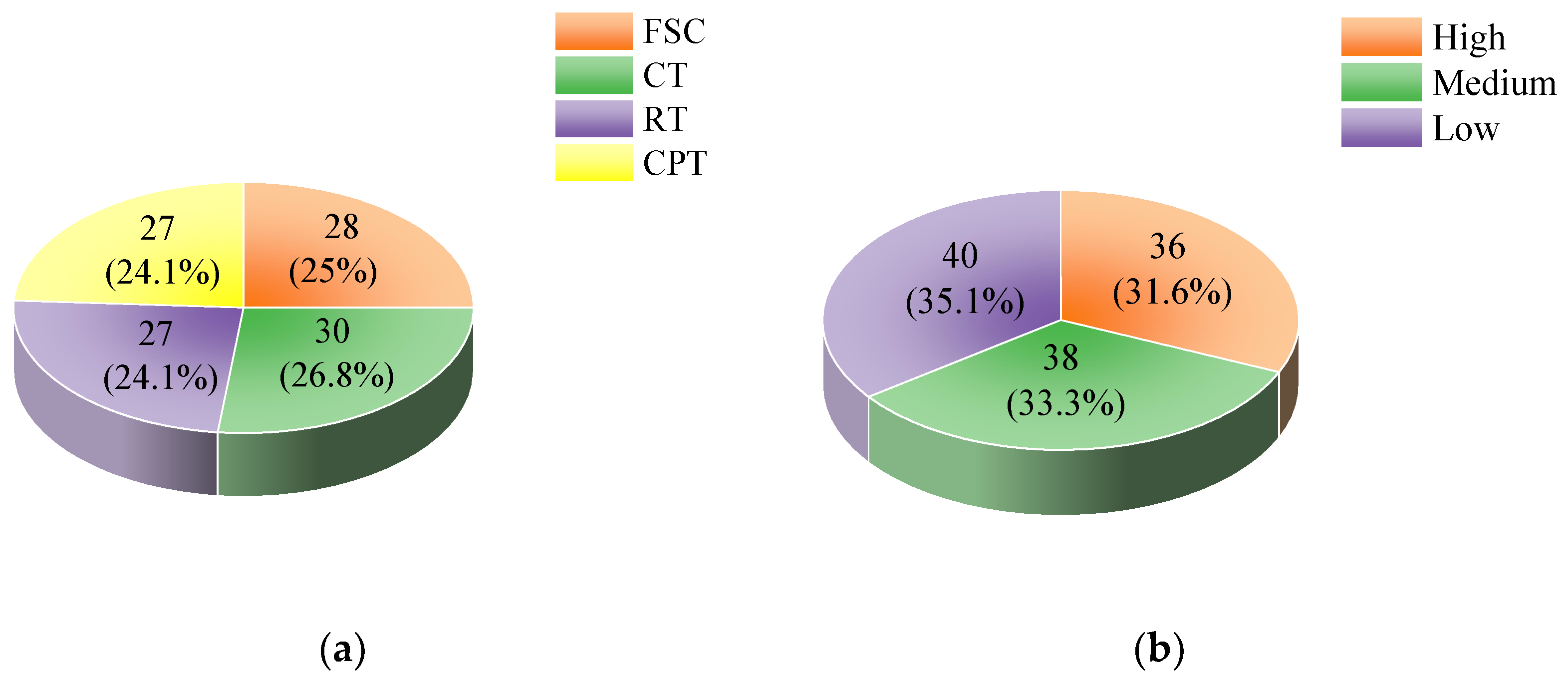
2.1. Sample Preparation

Soil from two distinct experimental fields affiliated with the Jilin Academy of Agricultural Sciences (JAAS) was selected as experimental samples. The first set comprised 112 soil samples subjected to four distinct treatments (tillage and straw management), while the other set contained 114 soil samples with a more spatially dispersed distribution. The JAAS is located in Gongzhuling City (43°5047′ N, 122°8576′ E), Jilin Province, and boasts fertile land resources and a diverse range of tillage practices. In addition, the obvious seasonal variation contributes to the deposition and storage of soil nutrients. To ensure the acquisition of relatively homogeneous soil samples, the plum-shaped sampling method was employed. At each point, five portions of tillage soil from depths of 5–20 cm were collected and thoroughly mixed. A 1 kg portion of this composite sample was subsequently hermetically sealed, labeled, and expeditiously transported to a laboratory for preservation under ambient conditions. Upon achieving a complete air-dry status, the samples were subjected to mashing, grinding, and sieving using a stone mortar, resulting in soil samples with dry particles smaller than 2 mm. In total, 30 g of the processed samples was used for testing according to the methodology in this paper, while the remaining samples were preserved for a chemical analysis, aiming to ascertain the major nutrient content of the soil to obtain the actual values.

2.2. Standards for Soil Classification

2.2.1. Soil Treatments

Within the defined research scope, soil samples were gathered without introducing additional confounding experimental factors, and 112 soil samples were collected under four treatments involving tillage and straw management including full straw coverage (FSC), conventional tillage (CT), rotational tillage (RT), and continuous plowing tillage (CPT) and obtained in the autumn of 2021. Further details of the treatments are presented in

Table 1. Detailed description of the four treatments.

Treatments	Treatment Details	Tillage and Straw Management
FSC	Full straw coverage	During harvesting in autumn, straw was pulverized (≤20 cm) and evenly spread. About a week before sowing, a straw-turning machine organized strip-like patterns (70–80 cm and 50–60 cm wide without straw). Seeding employed a no-till seeder in a wide–narrow row pattern, sowing seeds in the cleared 50–60 cm strip (40 cm seedbed width), and simultaneously applying base fertilizer.
CT	Conventional tillage	Mechanically harvested straw (≤20 cm) was baled and removed from the field pre-freezing. Approximately 20 days before sowing, a combined land leveling tool was used for stubble removal, rotary tillage, ridge formation, and fertilization. Compaction measures were applied for optimal sowing conditions. A precision seeder was then used for planting, followed by additional consolidation.
RT	Rotational tillage	In a corn–soybean rotation, straw was mechanically crushed during harvest. In autumn, a fence-type plow buried straw for incorporation, followed by harrowing for leveling. In spring, a secondary harrowing, contingent on surface conditions when soil thawed at 10 cm, achieved optimal sowing conditions.
CPT	Continuous plowing tillage	Mechanical harvest crushed and further pulverized straw. Pre-freezing, a fence-type five-share plow deeply tilled the field to 30–35 cm, followed by re-harrowing. The operation of spring sowing was the same as RT.

to aid in understanding the distribution and implications of each soil type on soil nutrient dynamics.

2.2.2. Soil Fertility Grades

The classification of soil fertility is conventionally grounded in the quantitative assessment of nutrient concentrations, with particular attention directed toward parameters encompassing carbon, nitrogen, phosphorus, potassium, and other indispensable nutrients present in the soil matrix. In this investigation, we conformed to the soil nutrient grading criteria stipulated in Beijing, China, selecting four fundamental indicators, namely, soil organic matter (SOM), total nitrogen (TN), available phosphorus (AP), and available potassium (AK). The scoring criteria for each index are delineated in

Table 2. Scoring rules for soil indicators.

Soil Nutrients	Score (F)	Extremely High	High	Medium	Low	Extremely Low
SOM	g/kg	≥25	25–20	20–15	15–10	<10
	value	100	80	60	40	20
TN	g/kg	≥1.20	1.20–1.00	1.00–0.80	0.80–0.65	<0.65
	value	100	80	60	40	20
AP	mg/kg	≥90	90–60	60–30	30–15	<15
	value	100	80	60	40	20
AK	mg/kg	≥155	155–125	125–100	100–70	<70
	value	100	80	60	40	20

. Conforming to the content magnitude of each index, a weight ratio of 0.3:0.25:0.25:0.2 was applied. The weight coefficients and scores allocated to the indices were subsequently employed in the computation of the integrated fertility index (IFI), with the explicit formula presented in Equation (1). Ultimately, 114 soil samples in this experimental study were stratified into distinct gradations, namely, “very high” (95–100), “high” (75–95), “medium” (50–75), “low” (30–50), and “very low” (0–30), where F_i is the score value of the i-th indicator and W_i is the weight of the i-th indicator. Illustratively, Figure 1 delineates the allocation of two sets of soil samples based on distinct classification criteria, facilitating a subsequent comprehension of the distribution and implications of each criterion on soil nutrient dynamics. The conspicuous observation is that the samples across various categories in both datasets exhibit a fairly uniform distribution, enhancing the feasibility of employing machine learning methodologies for the development of more robust classification models.

$$\mathrm{I}\mathrm{F}\mathrm{I}=\sum {\mathrm{F}}_{\mathrm{i}}\times {\mathrm{W}}_{\mathrm{i}}$$

(1)

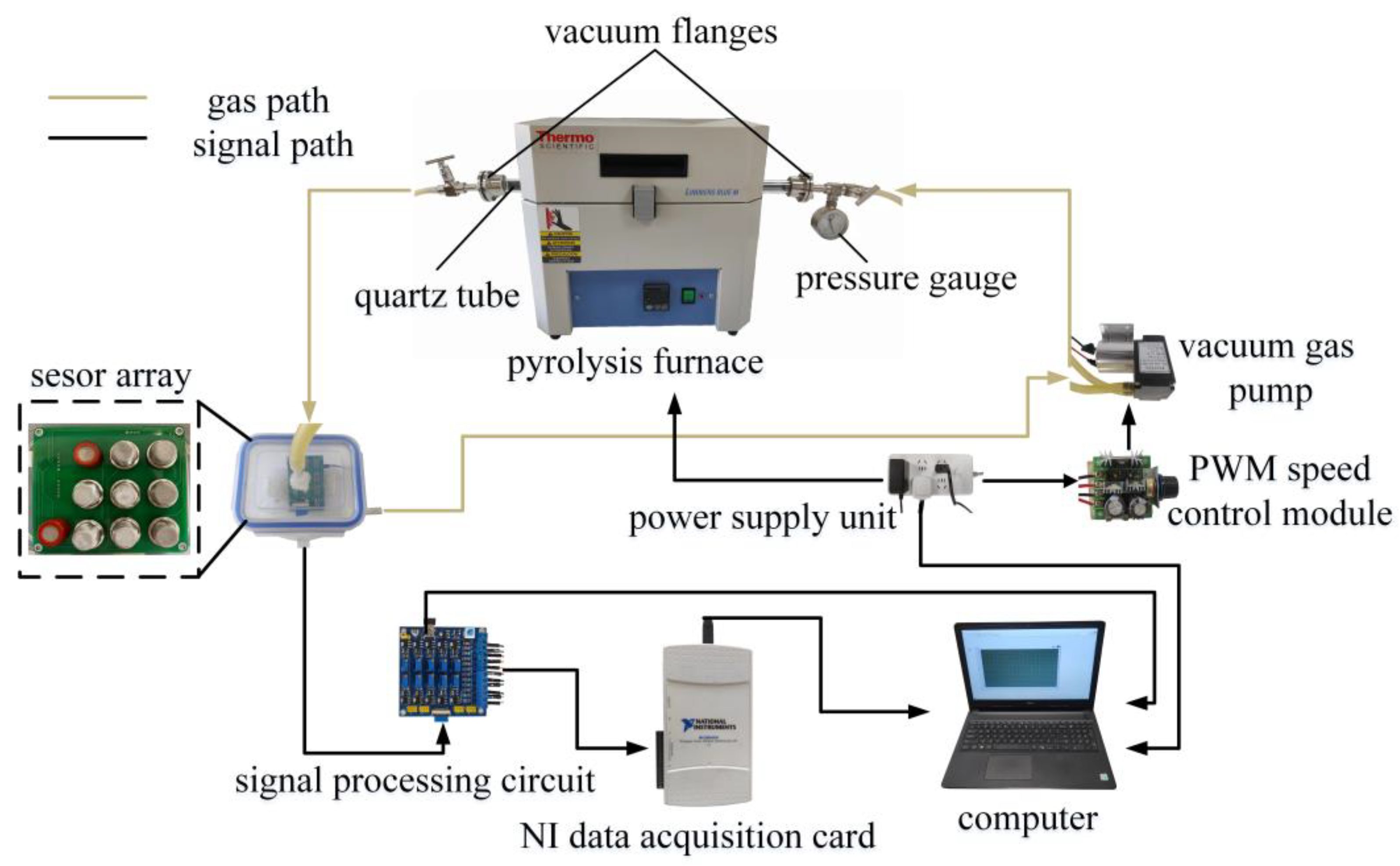
2.3. Machine Olfaction System

In this investigation, a soil detection system can be divided into a gas path and a signal path, including a power supply unit, a pyrolysis furnace, vacuum flanges, a quartz tube, a pressure gauge, a sensor array that accompanies a hermetic reaction chamber, a signal processing circuit, an NI data acquisition card, a computer, a PWM speed control module, and a vacuum gas pump being employed. As depicted in Figure 2, the pyrolysis furnace was used for high-temperature pyrolysis of soil samples. A quartz tube, with dimensions of 600 mm in length, 25 mm in outer diameter, and a wall thickness of 2.2 mm, was chosen as the pyrolysis chamber. A quartz boat was utilized to securely hold the soil samples, positioned at the central region of the quartz tube. The two ends of the quartz tubes were hermetically sealed with vacuum flanges, creating a sealed pyrolysis chamber to prevent external gas interference. Continuous monitoring of air pressure within the pyrolysis chamber was achieved through the utilization of a pressure gauge. Simultaneously, a pulse-width-modulated (PWM) module governed the flow rate of the vacuum gas pump, thereby facilitating the systematic circulation of the gas circuit encompassing the vacuum gas pump, the pyrolysis chamber, and the hermetically sealed reaction chamber. The soil pyrolysis gas was propelled into a hermetically sealed reaction chamber containing sensor arrays via a vacuum gas pump. Subsequently, the resultant sensor output signals underwent transmission to the host computer through a signal processing circuit and an NI data acquisition card. Notably, the signal processing circuit facilitated power supply to the sensor array and discerned alterations in gas concentration through the utilization of the resistor voltage division principle, converting such alterations into voltage output signals. The interconnection between the signal processing circuit and the NI data acquisition card was achieved via jumper wire, thereby affecting the transformation of analog signals into digital signals. Ultimately, the amassed sensor response data were conveyed to the Lab VIEW application on the computer through a USB data interface, thereby facilitating the presentation, storage, and subsequent data processing procedures.

2.4. Sensor Array Construction

MQ gas sensors have gained extensive usage in a wide range of machine olfaction studies, where their selectivity is reliant upon the gaseous products produced through the pyrolysis of the respective soil samples [41]. Elevated temperatures during pyrolysis intensify microbial activities in the soil, fostering the decomposition of compounds rich in carbon, nitrogen, phosphorus, sulfur, and other pertinent elements [42]. Numerous investigations have explored the decomposition process of these soil components and the subsequent release of gases. The gases formed during pyrolysis encompass carbon dioxide (CO₂), carbon monoxide (CO), alkanes, alcohols, nitrogen oxides (NO_x), ammonia (NH₃), sulfur dioxide (SO₂), and an array of volatile organic compounds (VOCs) [43,44,45]. Pertinent literature underscored the close correlation between the composition and concentration of gases produced during soil pyrolysis and factors such as the soil type and nutrient supply mechanisms. The precise makeup and quantity of these gases are subject to various influences, including the temperature, heating rate, soil type, and initial nutrient content. Consequently, variations in soil type and nutrient composition wield a notable influence on distinctions in the composition and concentration of pyrolytic gases, thereby impacting the strength of sensor output signals. We have engineered a sensor array characterized by pronounced sensitivity to gases emitted during soil pyrolysis, with specific emphasis on its reactivity to volatile compounds generated throughout the process. In-depth details regarding the specific types of gas sensors employed and associated parameters are presented in

Table 3. Specification of MOS sensors used in the designed sensor array.

Sensor No.	Sensor Type	Main Applications	Typical Detection Ranges (ppm)
S1	MQ-2	combustible gases, fumes	300–10,000
S2	MQ136	hydrogen sulfide (H2S)	1–200
S3	MQ131	ozone (O3)	10–1000
S4	MQ137	ammonia (NH3)	5–500
S5	MQ138	toluene, acetone, ethanol, hydrogen	5–500
S6	MQ-8	hydrogen (H2)	100–1000
S7	MQ-3B1	alcohol vapor	25–500
S8	MQ-4	methane (CH4)	300–10,000
S9	MQ-5	liquefied gas, methane, propane	300–10,000
S10	MQ-3B2	alcohol vapor	25–500

.

2.5. Data Acquisition

At the commencement of the experiment, 2 g of soil samples was accurately weighed and deposited onto a quartz boat. The quartz boat was then positioned at the central region of the quartz tube, and the vacuum flanges at both ends of the quartz tube were securely fastened to establish a sealed pyrolysis chamber. The tube pyrolysis furnace was activated, and the pyrolysis temperature was set to 400 °C. Once the designated temperature was attained, the pyrolysis furnace was opened, and the pre-prepared quartz tube was promptly positioned at the central locus within the pyrolysis furnace and swiftly sealed thereafter. Upon the restoration of temperature stability at 400 °C, initiate the formalized pyrolysis procedure, which persists for a duration of 3 min. Following the culmination of pyrolysis, the vacuum flanges on both sides were loosened, and the vacuum gas pump was set into operation with a flow rate of 1 L/min. Concurrently, the soil pyrolysis gas was directed into the enclosed reaction chamber. Owing to the activation of the gas path, the pyrolysis gas was pushed into the sealed reaction chamber housing the sensor array. Data acquisition was executed at a frequency of 10 Hz for a duration of 1 min. Upon the conclusion of data acquisition, the pyrolysis furnace was opened and the quartz tubes were subsequently taken out. The vacuum flanges situated at both ends were disassembled, allowing for the cooling, cleansing, and drying of the quartz tubes and quartz boats. Moreover, the flow rate of the vacuum gas pump was adjusted to 3 L/min to facilitate a 2 min cleaning procedure of the reaction gas path, wherein the experimental parameters were defined in accordance with methodologies delineated in prior research endeavors [46].

2.6. Eigenvalue Extraction

The gases obtained were converted into digital signals through a signal processing circuit and the NI data acquisition card, yielding raw data for each sensor. To mitigate the challenge of a possible “dimensionality disaster” resulting from the wealth of information within the raw response curves, a reduction in dimensionality was performed by extracting key eigenvalues. By following the principle of incorporating the most comprehensive set of eigenvalues, we extracted 9 eigenvalues from the initial response curves, including the seventh-second transient values (V_7s), initial values (V_IV), mean differential coefficient values (V_MDCV), mean values (V_MEAN), response area values (V_RAV), variance values (V_VV), maximum values (V_MAX), relative steady-state mean values (V_RSMV), and relative change values (V_RCV). Subsequently, these nine eigenvalues were employed to construct original eigenspaces with dimensions of 112 or 114 × 90 (112 or 114 samples × 10 sensors × 9 eigenvalues), wherein the calculation formulae are as follows:

$${\mathrm{V}}_{\mathrm{M}\mathrm{D}\mathrm{C}\mathrm{V}}=\frac{1}{\mathrm{N}-1}{\sum }_{\mathrm{i}}^{\mathrm{N}-1}\frac{{\mathrm{X}}_{\mathrm{i}+1}-{\mathrm{X}}_{\mathrm{i}}}{∆\mathrm{t}}$$

(2)

$${\mathrm{V}}_{\mathrm{M}\mathrm{E}\mathrm{A}\mathrm{N}}=\frac{\sum _{\mathrm{i}}^{\mathrm{N}}{\mathrm{X}}_{\mathrm{i}}}{\mathrm{N}}$$

(3)

$${\mathrm{V}}_{\mathrm{R}\mathrm{A}\mathrm{V}}={\sum }_{\mathrm{i}}^{\mathrm{N}}{\mathrm{X}}_{\mathrm{i}}∆\mathrm{t}$$

(4)

$${\mathrm{V}}_{\mathrm{V}\mathrm{V}}=\frac{{\sum }_{\mathrm{i}}^{\mathrm{N}}{({\mathrm{X}}_{\mathrm{i}}-\overline{\mathrm{X}})}^2}{\mathrm{N}}$$

(5)

$${\mathrm{V}}_{\mathrm{R}\mathrm{S}\mathrm{M}\mathrm{V}}=\frac{{\sum }_{\mathrm{i}={\mathrm{t}}_0}^{\mathrm{T}}{\mathrm{X}}_{\mathrm{i}}}{\mathrm{T}-{\mathrm{t}}_0}$$

(6)

$${\mathrm{V}}_{\mathrm{R}\mathrm{C}\mathrm{V}}=\frac{{\mathrm{X}}_{\mathrm{e}\mathrm{n}\mathrm{d}}-{\mathrm{X}}_0}{\mathrm{T}}$$

(7)

Here, X₀, X_i, $\overline{\mathrm{X}}$, and X_end represent the initial, first, average, and end values of the sensor data, respectively. The value N signifies the number of data points measured with a sensor, while t₀ denotes the time corresponding to the moment when a steady state is achieved. The acquisition time is denoted by T (70 s), and $∆\mathrm{t}$ represents the time interval between two consecutive sampling points (0.1 s). Additionally, it is noteworthy that transient response values may encompass supplementary information reflective of the real-time dynamic behavior of the sensor.

2.7. Feature Space Optimization

The initial feature space necessitates the elimination of redundant or inconsequential features through the identification and selection of the most pertinent and predictive variables. Mutual information (MI) was employed as a metric for quantifying the extent of information exchange between two variables [47,48]. Given the presence of obscure linear or nonlinear interrelationships in the original feature space, MI endeavors to identify diverse intricate relationships among variables, extending beyond the confines of linear correlation measurement. Consider the presence of random variables X and Y, wherein X represents the feature, and Y represents the target variable. The expression for MI is articulated as follows:

$$\mathrm{M}\mathrm{I}(\mathrm{X},\mathrm{Y})=\sum _{\mathrm{x}\in \mathrm{X}}\sum _{\mathrm{y}\in \mathrm{Y}}\mathrm{P}(\mathrm{X},\mathrm{Y}){\log }_2\left[\mathrm{P}(\mathrm{X},\mathrm{Y})/\mathrm{P}\left(\mathrm{X}\right)\mathrm{P}\left(\mathrm{Y}\right)\right]$$

(8)

Herein, P (X, Y) signifies the joint probability distribution of random variables X and Y, while P (X) and P (Y) denote the marginal probability distributions of X and Y, respectively. The magnitude of MI (X, Y) is directly proportional to the strength of the correlation between X and Y.

2.8. Classification Models

Classification models constitute a vital category of tasks within the realm of machine learning, characterized by their principal objective of categorizing input data into distinct classes or labels, applicable to the domain of agriculture. To partition the dataset into training and test sets for model fitting and evaluation, the Kennard–Stone (K-S) algorithm was employed [49]. Specifically, a ratio of 6:4 was applied to allocate 112 soil samples and 114 soil samples, respectively, based on two classification criteria. To optimize the classification of the dataset, three advanced machine learning algorithms—RF, multi-layer perceptron (MLP), and a hybrid MLP-RF model—were employed. The comparative analysis of these algorithms was geared toward identifying the most effective classification model, taking into account their respective capabilities in accurately categorizing the soil sample data.

2.8.1. RF Classification Model

RF functions as an ensemble learning method, employing multiple decision trees. This algorithm introduces randomness in the selection of training samples and the features considered at each node of the trees. Each tree is constructed independently, and the final prediction is determined by aggregating the predictions of all individual trees. The deliberate introduction of diversity within the decision trees allows RF to often achieve increased accuracy by mitigating overfitting and improving generalization [50]. Additionally, RF’s versatility in handling various features facilitates the integration of diverse soil properties and attributes, thereby enhancing its effectiveness in comprehensive soil classification [51].

2.8.2. MLP Classification Model

The MLP model employs the backpropagation algorithm to iteratively adjust weights, minimizing the discrepancy between predicted and actual outputs. Structurally, MLP is comprised of a stratification of neurons organized across several layers, encompassing an input layer, one or multiple hidden layers, and an output layer, and the performance depends on its structure (number of layers and neurons), the weight optimization process, and the choice of activation functions [52]. The inherent capability for learning intricate patterns within the data enhances its efficacy in discerning diverse soil classes based on multidimensional input features. The adaptive learning process facilitates the refinement of internal representations, enabling robust modeling of the intricate relationships inherent in soil properties [53].

2.8.3. MLP-RF Classification Model

The amalgamation of MLP and RF models constitutes a sophisticated integrated learning strategy, and this approach strategically weighs and amalgamates the predictions from both models. The construction of the final classifier involves an iterative synthesis of models and weights, which is orchestrated to recalibrate sample weights. The hybrid model excels in integrating diverse soil features, accommodating both linear and nonlinear relationships among soil properties [54]. The ensemble learning from RF, coupled with the ability of MLP to capture intricate patterns, enhances the accuracy of soil classification tasks.

2.9. Model Evaluation Indicators

Employing evaluation metrics for classification models serves the purpose of gauging their efficacy across diverse classification tasks. Widely employed metrics such as overall accuracy (OA) and the Kappa coefficient play pivotal roles in the evaluation of classification model performance, which provides an integrated assessment of model performance [55,56], and their mathematical expressions are as in Equations (9) and (10). Here, CS denotes the number of correctly classified samples, while TS signifies the total number of samples under the dataset. The E(OA) encapsulates the anticipated value of OA, which is derived through a calculation contingent upon the inherent category distribution within the dataset when devoid of any modeling influence.

The OA stands out as an instinctive metric employed in the evaluation of classification model performance. In concrete terms, OA is computed as the ratio of correctly classified samples to the total number of samples. The proximity of its value to 100% signifies a superior performance of the model, whereas the Kappa coefficient serves as a metric that accounts for the inherent stochastic nature of a classification model. It quantifies the degree of error reduction between the model’s classification and a completely random classification, indicating the underlying consistency between the obtained results and the true reference. Typically confined to the range of 0 to 1, the Kappa coefficient undergoes categorization into distinct groups denoting varying degrees of consistency: 0.00–0.20 (extremely low), 0.21–0.40 (fair), 0.41–0.60 (moderate), 0.61–0.80 (substantial), and 0.81–1.00 (almost perfect). A Kappa coefficient of 1 denotes perfect consistency, signifying that the classification outcome aligns impeccably with the actual situation. Within the realm of classification, the attainment of peak performance using a classification model is evidenced by the OA nearing 100% and the Kappa coefficient converging toward 1. The optimal classification model for the current task was discerned through a thorough evaluation utilizing OA and the Kappa coefficient as dual evaluative indicators.

$$\mathrm{O}\mathrm{A}=\frac{\mathrm{C}\mathrm{S}}{\mathrm{T}\mathrm{S}}\times 100\mathrm{\%}$$

(9)

$$\mathrm{K}\mathrm{a}\mathrm{p}\mathrm{p}\mathrm{a}=\frac{\mathrm{O}\mathrm{A}-\mathrm{E}\left(\mathrm{O}\mathrm{A}\right)}{1-\mathrm{E}\left(\mathrm{O}\mathrm{A}\right)}$$

(10)

3. Results and Discussion

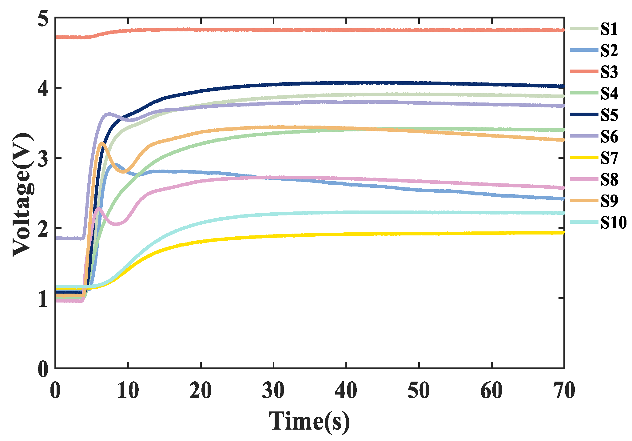
3.1. Output Signal Acquisition

The implemented detection system captures output signals at distinct phases of the soil pyrolysis process. As the soil pyrolysis gas permeates into the reaction chamber housing the sensor array, the sensor response curve exhibits a swift ascent concurrent with the gas filling, eventually attaining a stabilized state within a defined range. Figure 3 illustrates the responsiveness of the sensor array to pyrolysis gases emitted by the soil, showcasing a notable divergence in the output signals among the various sensors.

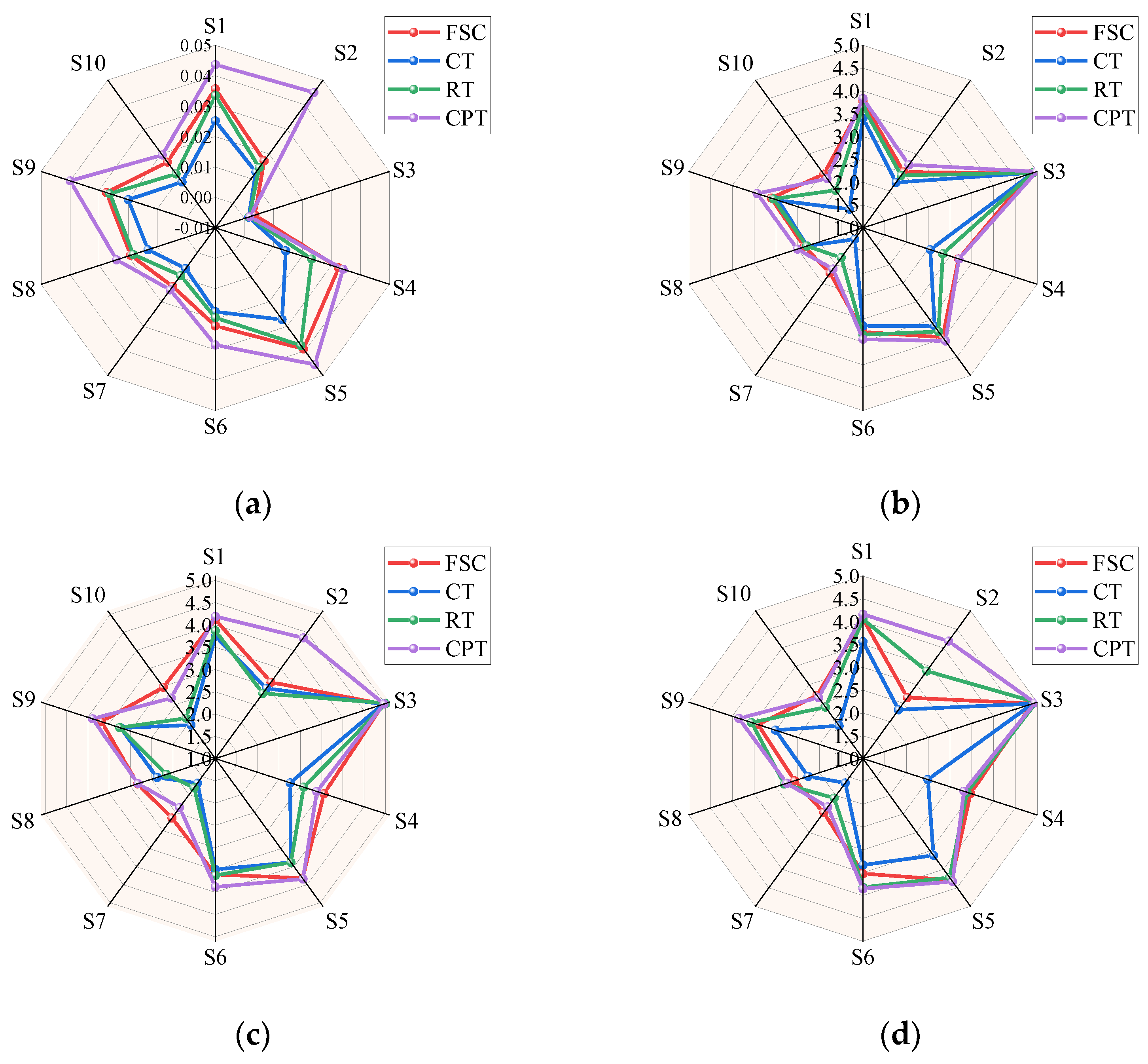
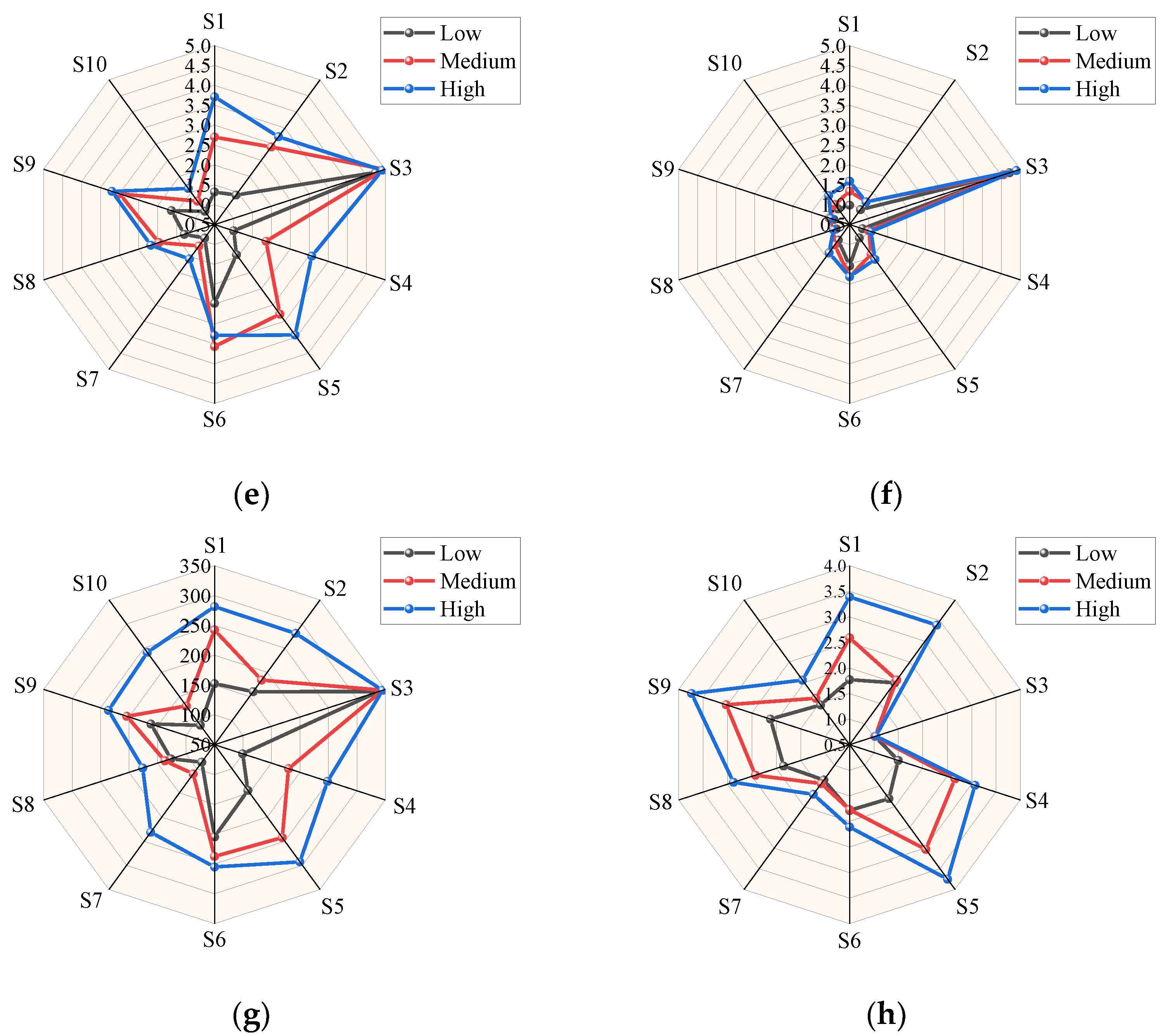
3.2. Feature Space Construction

The experimental setup incorporated 10 gas sensors, from which nine distinctive feature parameters were derived for each sensor response curve. Consequently, two original feature space matrices of dimensions 112 × 10 × 9 and 114 × 10 × 9 were constructed, representing the datasets derived from 112 or 114 soil samples, 10 sensors, and 9 feature parameters in each case. Figure 4 illustrates a radar plot delineating the disparities in the response, specifically focusing on representative eigenvalues derived from the output responses of diverse sensors. The differential responsivity of individual sensors to distinct soil classes induces disparate gas stimulation patterns within the sensor array. This point suggests substantiation with the discernible differences in the characteristics of pyrolysis gas from soil, highlighting the discriminative capacity of the machine olfaction technique in distinguishing between sample odors.

As evidenced by Figure 4a–d, radar plots representing the response eigenvalues of soils subjected to four distinct treatments reveal a consistent shape, with variations in specific values. Notably, with the exception of sensor S3, soil treatment involving CPT stands out, demonstrating elevated levels of response eigenvalues. This phenomenon can be attributed to the soil disturbance and fragmentation inherent in CPT, fostering intricate interactions between organic matter and soil microorganisms. In contrast, CT involving mechanical straw crushing posed challenges in reintegrating organic matter into farmland, impacting soil compaction, aeration, and subsequently nutrient distribution. Altered soil physical properties may affect nutrient distribution within the soil profile, potentially contributing to lower eigenvalues in CT. The distinction between FSC and RT was less pronounced. FSC involved the preservation of surface vegetation and straw, minimizing soil disturbance to enhance nutrient retention, primarily in the surface layer. RT, promoting nutrient cycling through plant residue alternation, may require increased availability of phosphorus and potassium, influencing soil salt solubility. While the non-uniform dispersion of nutrients in both FSC and RT rendered their eigenvalues comparably lower than those observed in the context of CPT, discernible differences persist under specific sensors, such as S2 and S7 under V_RAV.

The discernable variations in response eigenvalues among soils stratified into three distinct fertility classes are prominently depicted in Figure 4e–h. Evidently, there exists a positive correlation between higher fertility classes and increased response eigenvalues in the soils. This observation substantiates the conjecture that variations in the concentration of volatile organic compounds induce alterations in the responses of the sensor array.

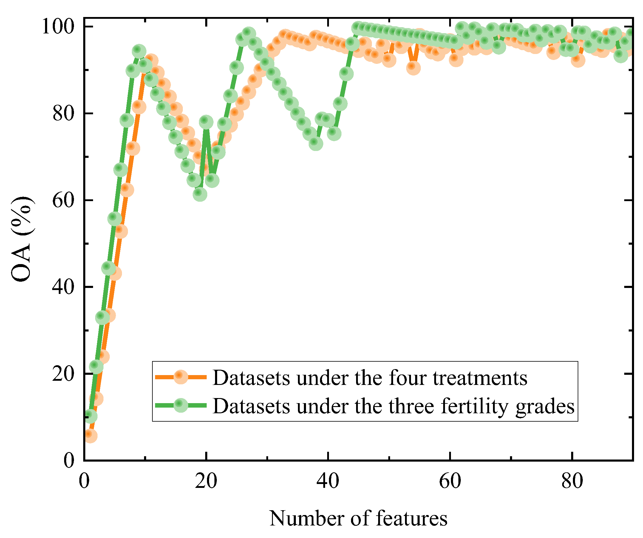
3.3. Feature Space Optimization Results

In the application of MI for feature selection within the foundational feature space, dedicated classification models were devised for the two discrete soil classification criteria by incorporating the RF algorithm. The criterion for feature selection was established upon maximizing the OA. Acknowledging the inherent stochastic properties of the RF algorithm and the instability of the fitting procedure, the present study undertook 10 iterations of averaging on the two initial feature matrices to mitigate potential ramifications of random sampling, as illustrated in Figure 5. It is evident that the cumulative accuracy of the two classification models exhibited a progressive increase as the number of features escalated until it eventually stabilized within a particular range. The OA attained its apex when the number of features reached 67 and 62, respectively. It was thus deemed appropriate to preserve 67 and 62 features to obtain the ultimate optimized feature space.

3.4. Modeling Results

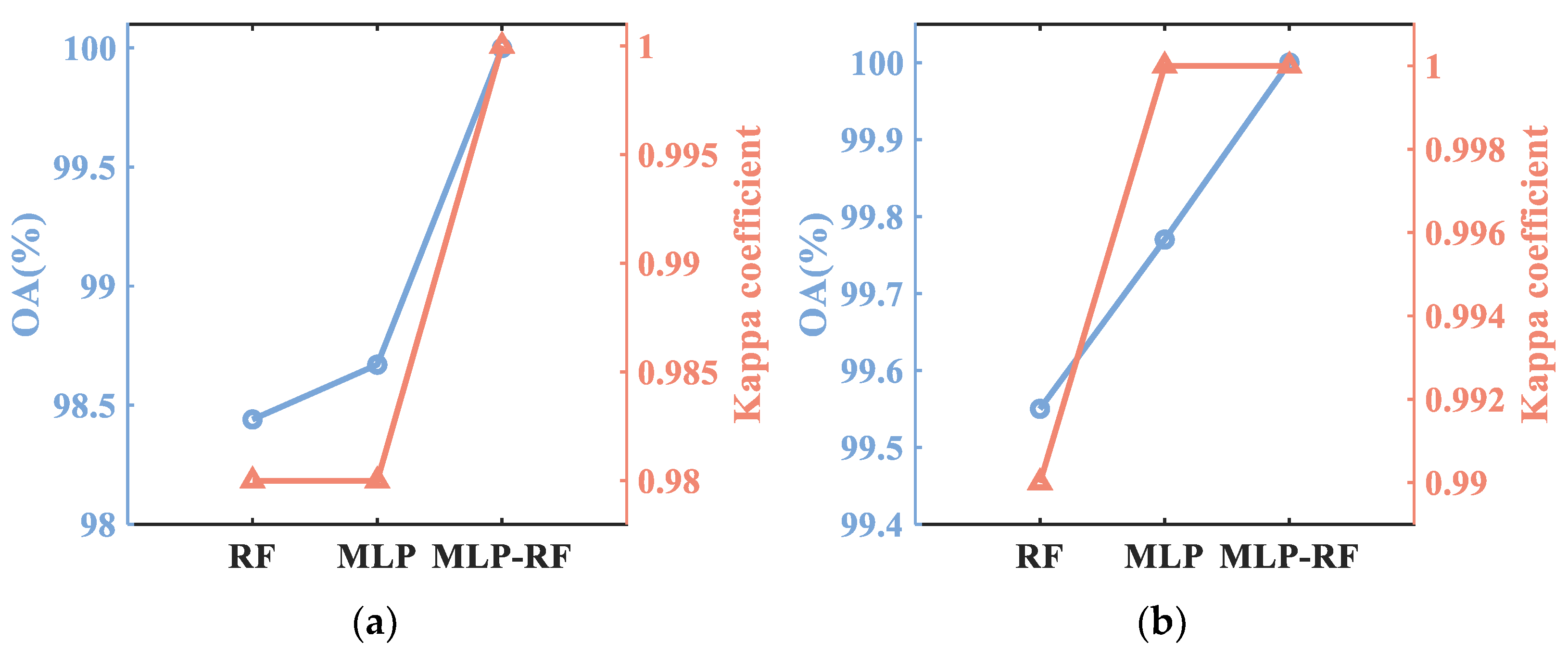
3.4.1. Modeling Performance

The ultimate modeling strategy was carried out based on the optimized feature space, and the evaluation of classification outcomes under both criteria was conducted, employing three learning models. In this particular scenario, the RF classification model was configured with 150 decision trees, a minimum leaf size of 2, and unrestricted tree depth to facilitate maximal growth. The MLP model comprised two hidden layers, encompassing 16 neurons, with a specified maximum iteration count of 70 and a mini-batch size of 12. The amalgamation of the basic learners into the MLP-RF classification model was achieved by encapsulating them in a single-element string. Subsequently, weights were assigned to the MLP and RF learners, with MLP weights set at 0.7 and RF weights set at 0.3, with a designated learning period of 50. Upon parameter adjustment and configuration through cross-validation, a discrimination analysis was conducted on two distinct datasets acquired from ten sensors. The iterative execution of each algorithm, performed in a repeated manner for a total of ten trials, was designed to alleviate the influence of random variables, thereby guaranteeing the attainment of reliable outcomes. Also, the confusion matrix obtained by using the proposed algorithm is given in

Table 4. The confusion matrix resulting from the classification of soils under four treatments using the RF model.

Soil Treatments	Number of Test Samples	Predicted				Classification Accuracy (%)
		FSC	CT	RT	CPT
FSC	110	108	0	2	0	98.18
CT	120	0	118	2	0	98.33
RT	110	3	0	107	0	97.27
CPT	110	0	0	0	110	100.00

,

Table 5. The confusion matrix resulting from the classification of soils under four treatments using the MLP model.

Soil Treatments	Number of Test Samples	Predicted				Classification Accuracy (%)
		FSC	CT	RT	CPT
FSC	110	107	0	2	1	97.27
CT	120	0	119	1	0	99.17
RT	110	2	0	108	0	98.18
CPT	110	0	0	0	110	100.00

,

Table 6. The confusion matrix resulting from the classification of soils under four treatments using the MLP-RF model.

Soil Treatments	Number of Test Samples	Predicted				Classification Accuracy (%)
		FSC	CT	RT	CPT
FSC	110	110	0	0	0	100.00
CT	120	0	120	0	0	100.00
RT	110	0	0	110	0	100.00
CPT	110	0	0	0	110	100.00

,

Table 7. The confusion matrix resulting from the classification of soils under three fertility grades using the RF model.

Soil Fertility Grades	Number of Test Samples	Predicted			Classification Accuracy (%)
		Low	Medium	High
Low	130	130	0	0	100.00
Medium	150	0	149	1	99.33
High	160	0	1	159	99.38

,

Table 8. The confusion matrix resulting from the classification of soils under three fertility grades using the MLP model.

Soil Fertility Grades	Number of Test Samples	Predicted			Classification Accuracy (%)
		Low	Medium	High
Low	130	130	0	0	100.00
Medium	150	0	149	1	99.33
High	160	0	0	160	100.00

and

Table 9. The confusion matrix resulting from the classification of soils under three fertility grades using the MLP-RF model.

Soil Fertility Grades	Number of Test Samples	Predicted			Classification Accuracy (%)
		Low	Medium	High
Low	130	130	0	0	100.00
Medium	150	0	150	0	100.00
High	160	0	0	160	100.00

.

Table 4, Table 5 and Table 6 reveal that, among soils subjected to four distinct treatments, CPT exhibited the utmost classification accuracy, achieving a flawless 100% accuracy across all three models. This exceptional performance was ascribed to the superior response output values associated with CPT. During the classification task, it was observed that the test points for the FSC and RT models exhibited notable confusion. This observation was further supported by the evidence depicted in Figure 4a,b, which demonstrates the presence of an overlap in the output eigenvalues (V_MDCV, V_MEAN) obtained from both sensors. This observation substantiates the hypothesis positing a non-uniform distribution of nutrients in both FSC and RT. Concerning CT, when subjected to classification under the RF and MLP models, a minor fraction of samples were misclassified into the RT category. Despite the conspicuous dissimilarity between CT and the other three treatments evident in Figure 4a,d, the nature of the subtle overlap in eigenvalues between CT and RT persists, as illustrated in Figure 4c. Owing to the limited sample size, the misclassification of a small fraction of sample points exerted a discernible influence on classification accuracy. Nonetheless, the RF model and MLP model both attained classification accuracy surpassing 97.00%, facilitating the fundamental achievement of soil classification under the four treatments. Similar results were obtained in the classification of multiple soil samples by Nguyen et al. [57]. In a comparative analysis, the amalgamated MLP-RF model exhibited the utmost classification accuracy, achieving a comprehensive and accurate classification of soil under all four treatment modalities. As expected, the classification of the three fertility grades demonstrated a generally satisfactory performance, with only a few misclassified samples observed in the RF and MLP models, particularly within the “medium” and “high” fertility classes. The chosen soil sampling locations were relatively dispersed. However, it is crucial to note that these sampling areas were inherently part of the same farmland. The misclassifications observed can be attributed to the inherent similarity in nutrient structure across the sampled regions. Comparable outcomes were documented by Wang and Chen et al. in their assessment of the capability of machine olfaction techniques for discerning gas mixtures [58,59].

3.4.2. Modeling Evaluation

Utilizing OA and Kappa coefficients, a comprehensive evaluation of the three classification models was conducted under the two soil classification criteria. The classification evaluation indices are presented in Figure 6. Upon employing a consistent feature space optimization method, it is observed that the MLP-RF model demonstrates superior performance. The OA in soil classification for distinct treatments and fertility classes attains 100%, accompanied by corresponding Kappa coefficients of 1.00.

Among the considered models, the RF model may exhibit suboptimal performance in the presence of intricate nonlinear relationships, yielding OA of 98.44% and 99.55%, accompanied by Kappa coefficients of 0.98 and 0.99, respectively, under the two distinct classification criteria. Despite the apparent limitation in interpretability, the RF model effectively accomplishes the soil classification task, producing classification outcomes that closely align with the actual results. On the other hand, the MLP model may exhibit a predisposition toward overfitting, particularly when confronted with a limited training dataset. The OA metrics for the MLP model, computed with respect to the two distinct classification criteria, recorded values of 98.67% and 99.77%, while the corresponding Kappa coefficients were determined to be 0.98 and 1.00, respectively. Although instances of isolated misclassification errors were observed, the resultant classification outcomes remained proximal to the idealized perfect state, being particularly noteworthy when applied to the classification of soils into three distinct fertility classes. This observed closeness underscores the model’s resilience in the context of limited data availability. The superiority of the MLP-RF model can be attributed to several factors; by amalgamating these models, the risk of overfitting is mitigated, enabling a more comprehensive capture of patterns within complex data. Given that MLP and RF excel at capturing distinct types of data, the amalgamated model achieves a more comprehensive depiction of features and relationships within complex data. This contributes to an enhanced overall understanding of the dataset and enhances the model’s generalization ability and classification accuracy. The findings substantiated the research revealing that the hybrid model surpasses conventional methodologies with respect to classification accuracy across diverse soil types [60]. Overall, our findings indicate that the MLP-RF model demonstrates superior performance on both classification criteria, displaying unbiased effectiveness across all categories. Furthermore, the classification outcomes under both criteria exhibit perfect consistency with the actual results.

4. Conclusions

Within this research endeavor, a soil classification apparatus grounded in pyrolysis and machine olfaction was conceptualized, employing a sensor array comprising ten gas sensors. This ensemble facilitated the surveillance of gas mixtures emanating from soil pyrolysis as well as variations in their concentrations. Upon the derivation of feature metrics from the sensor response curves, an optimization procedure leveraging mutual information was employed to mitigate feature redundancy within the feature space. Subsequently, the discriminatory efficacy of three distinct machine learning methodologies, namely, RF, MLP, and a hybrid MLP-RF, was systematically evaluated across soils subjected to varied treatments and diverse fertility gradients. The performance evaluation encompassed the utilization of well-established metrics, including OA and Kappa coefficients, to ascertain the efficacy and robustness of the predictive models. The experimental results demonstrate that the classification ability of the models follows a recursive pattern, with MLP-RF outperforming MLP and RF. Particularly, the MLP-RF model exhibited commendable discriminatory capabilities under both classification criteria, achieving an impeccable OA coupled with a Kappa coefficient, thus highlighting significant congruence with actual data. The superior performance of MLP-RF can be attributed, to some extent, to its integration of multiple learning algorithms. Such a synergistic learning strategy not only augments the overall predictive performance but also attenuates the inherent constraints intrinsic to singular model architectures, thereby furnishing a robust framework for advancing soil classification research.

In the realm of soil management, the spatial configuration of soil nutrient distribution exhibits a pronounced association with the gas composition resulting from soil pyrolysis processes. The method delineated machine olfaction as a dependable means for the expeditious and effective classification of soils. This holds particularly true when forecasting unknown soil samples, obviating the necessity for labor-intensive experimental procedures. Furthermore, the methodology proposed in this study can not only be applied to evaluate a wide range of soil characteristics but also warrants further investigation, particularly in the intricate field of soil contamination.

References

1. Williams, H.; Colombi, T.; Keller, T. The influence of soil management on soil health: An on-farm study in southern Sweden. Geoderma 2020, 360, 114010. [Google Scholar] [CrossRef]
2. Lehman, R.; Osborne, S.; McGraw, K. Stacking Agricultural Management Tactics to Promote Improvements in Soil Structure and Microbial Activities. Agronomy 2019, 9, 539. [Google Scholar] [CrossRef]
3. Zhao, H.; Wu, L.; Zhu, S.; Sun, H.; Xu, C.; Fu, J.; Ning, T. Sensitivities of Physical and Chemical Attributes of Soil Quality to Different Tillage Management. Agronomy 2022, 12, 1153. [Google Scholar] [CrossRef]
4. Fors, R.; Sorci-Uhmann, E.; Santos, E.; Silva-Flores, P.; Abreu, M.; Viegas, W.; Nogales, A. Influence of Soil Type, Land Use, and Rootstock Genotype on Root-Associated Arbuscular Mycorrhizal Fungi Communities and Their Impact on Grapevine Growth and Nutrition. Agriculture 2023, 13, 2163. [Google Scholar] [CrossRef]
5. Potapov, A.; Beaulieu, F.; Birkhofer, K.; Bluhm, S.; Degtyarev, M.; Devetter, M.; Goncharov, A.; Gongalsky, K.; Klarner, B.; Korobushkin, D. Feeding habits and multifunctional classification of soil-associated consumers from protists to vertebrates. Biol. Rev. 2022, 97, 1057–1117. [Google Scholar] [CrossRef] [PubMed]
6. Kim, W.; Lee, D.; Kim, T.; Kim, G.; Kim, H.; Sim, T.; Kim, Y. One-shot classification-based tilled soil region segmentation for boundary guidance in autonomous tillage. Comput. Electron. Agric. 2021, 189, 106371. [Google Scholar] [CrossRef]
7. Lee, D.; Kim, Y.; Sonn, Y.; Kim, K. Comparison of Soil Taxonomy (2022) and WRB (2022) Systems for Classifying Paddy Soils with Different Drainage Grades in South Korea. Land 2023, 12, 1204. [Google Scholar] [CrossRef]
8. Li, Y.; Wu, J.; Wang, Y.; Hu, Y. Precision agriculture technologies for sustaining smallholder farming systems. J. Integr. Agric. 2019, 18, 771–781. [Google Scholar]
9. Xu, J.; Han, H.; Ning, T.; Li, Z.; Lal, R. Long-term effects of tillage and straw management on soil organic carbon, crop yield, and yield stability in a wheat-maize system. Eur. J. Agron. 2019, 233, 33–40. [Google Scholar] [CrossRef]
10. Mutuku, E.; Vanlauwe, B.; Roobroeck, D.; Boeckx, P.; Cornelis, W. Physico-chemical soil attributes under conservation agriculture and integrated soil fertility management. Nutr. Cycl. Agroecosyst. 2021, 120, 145–160. [Google Scholar] [CrossRef]
11. Smith, J.; Johnson, A.; Doe, R. Advances in Soil Assessment Techniques. Soil Sci. Soc. Am. J. 2015, 79, 714–725. [Google Scholar]
12. Jones, M.; White, K.; Robinson, P. Real-time Soil Monitoring Technologies: A Review. Environ. Sci. Technol. 2018, 52, 7719–7732. [Google Scholar]
13. Brown, C.; Miller, E.; Davis, R. Enhancing Spatial Resolution in Large-Scale Soil Testing through Advanced Classification Methods. J. Agric. Sci. 2020, 10, 112–124. [Google Scholar]
14. Maynard, J.; Salley, S.; Beaudette, D.; Herrick, J. Numerical soil classification supports soil identification by citizen scientists using limited, simple soil observations. Soil Sci. Soc. Am. J. 2020, 84, 1675–1692. [Google Scholar] [CrossRef]
15. Vibhute, A.; Kale, K.; Gaikwad, S. Machine learning-enabled soil classification for precision agriculture: A study on spectral analysis and soil property determination. Appl. Geomat. 2024. [Google Scholar] [CrossRef]
16. Xu, H.; Xu, D.; Chen, S.; Ma, W.; Shi, Z. Rapid Determination of Soil Class Based on Visible-Near Infrared, Mid-Infrared Spectroscopy and Data Fusion. Remote Sens. 2020, 12, 1512. [Google Scholar] [CrossRef]
17. Hark, R.; Throckmorton, C.; Harmon, R.; Plumer, J.; Harmon, K.; Harrison, J.; Hendrickx, J.; Clausen, J. Multianalyzer Spectroscopic Data Fusion for Soil Characterization. Appl. Sci. 2020, 10, 8723. [Google Scholar] [CrossRef]
18. Duan, M.Q.; Zhang, X.G. Using remote sensing to identify soil types based on multiscale image texture features. Comput. Electron. Agric. 2021, 187, 106272. [Google Scholar] [CrossRef]
19. Zhang, W.; Zhu, L.; Zhuang, Q.; Chen, D.; Sun, T. Mapping Cropland Soil Nutrients Contents Based on Multi-Spectral Remote Sensing and Machine Learning. Agriculture 2023, 13, 1592. [Google Scholar] [CrossRef]
20. Haugen, H.; Devineau, O.; Heggenes, J.; Ostbye, K.; Linlokken, A. Predicting Habitat Properties Using Remote Sensing Data: Soil pH and Moisture, and Ground Vegetation Cover. Remote Sens. 2022, 14, 5207. [Google Scholar] [CrossRef]
21. Wang, Y.; Huang, H.; Chen, X. Predicting Organic Matter Content, Total Nitrogen and pH Value of Lime Concretion Black Soil Based on Visible and Near Infrared Spectroscopy. Eurasian Soil Sci. 2021, 54, 1681–1688. [Google Scholar] [CrossRef]
22. Carrillo, V.; Heenkenda, M.; Nelson, R.; Sahota, T.; Serrano, L. Deep learning in land-use classification and geostatistics in soil pH mapping: A case study at Lakehead University Agricultural Research Station, Thunder Bay, Ontario, Canada. J. Appl. Remote Sens. 2022, 16, 034519. [Google Scholar] [CrossRef]
23. Seesaard, T.; Goel, N.; Kumar, M.; Wongchoosuk, C. Advances in gas sensors and electronic nose technologies for agricultural cycle applications. Comput. Electron. Agric. 2022, 193, 106673. [Google Scholar] [CrossRef]
24. Okur, S.; Sarheed, M.; Huber, R.; Zhang, Z.J.; Heinke, L.; Kanbar, A.; Woll, C.; Nick, P.; Lemmer, U. Identification of Mint Scents Using a QCM Based E-Nose. Chemosensors 2021, 9, 31. [Google Scholar] [CrossRef]
25. Wesoly, M.; Przewodowski, W.; Ciosek-Skibinska, P. Electronic noses and electronic tongues for the agricultural purposes. Trac-Trends Anal. Chem. 2023, 164, 117082. [Google Scholar] [CrossRef]
26. Khorramifar, A.; Karami, H.; Wilson, A.D.; Sayyah, A.H.A.; Shuba, A.; Lozano, J. Grape Cultivar Identification and Classification by Machine Olfaction Analysis of Leaf Volatiles. Chemosensors 2022, 10, 125. [Google Scholar] [CrossRef]
27. Bieganowski, A.; Jaromin-Glen, K.; Guz, Ł.; Łagód, G.; Jozefaciuk, G.; Franus, W.; Suchorab, Z.; Sobczuk, H. Evaluating Soil Moisture Status Using an e-Nose. Sensors 2016, 16, 886. [Google Scholar] [CrossRef] [PubMed]
28. Lavanya, S.; Krishna Murthy, V. Suitability of Electronic Nose as a Reflective Tool to the Measurement of Soil Fertility Factors. Eng. Technol. 2018, 13, 39–47. [Google Scholar] [CrossRef]
29. Ba, F.; Peng, P.; Zhang, Y.; Zhao, Y. Classification and Identification of Contaminants in Recyclable Containers Based on a Recursive Feature Elimination-Light Gradient Boosting Machine Algorithm Using an Electronic Nose. Micromachines 2023, 14, 2047. [Google Scholar] [CrossRef] [PubMed]
30. Yu, D.B.; Gu, Y. A Machine Learning Method for the Fine-Grained Classification of Green Tea with Geographical Indication Using a MOS-Based Electronic Nose. Foods 2021, 10, 795. [Google Scholar] [CrossRef] [PubMed]
31. Tian, H.; Liu, H.; He, Y.; Chen, B.; Xiao, L.; Fei, Y.; Wang, G.; Yu, H.; Chen, C. Combined application of electronic nose analysis and back-propagation neural network and random forest models for assessing yogurt flavor acceptability. J. Food Meas. Charact. 2020, 14, 573–583. [Google Scholar] [CrossRef]
32. Barman, U.; Choudhury, D. Soil texture classification using multi class support vector machine. Inf. Process. Agric. 2020, 7, 318–332. [Google Scholar] [CrossRef]
33. Zhang, J.; Wang, J.; Zhou, X. Soil organic matter content classification based on random forest algorithm. J. Resour. Ecol. 2019, 9, 542–548. [Google Scholar]
34. Mouazen, A.M.; Alhwaimel, S.A.; Kuang, B.; Waine, T. Multiple on-line soil sensors and data fusion approach for delineation of water holding capacity zones for site specific irrigation. Soil Tillage Res. 2014, 143, 95–105. [Google Scholar] [CrossRef]
35. Zhang, Y.; Wei, Z.; Xie, Y. Texture analysis in soil moisture mapping using satellite imagery. Remote Sens. 2018, 10, 789. [Google Scholar]
36. LeCun, Y.; Bengio, Y.; Hinton, G. Deep learning. Nature 2015, 521, 436–444. [Google Scholar] [CrossRef]
37. Graves, A.; Schmidhuber, J. Framewise phoneme classification with bidirectional LSTM and other neural network architectures. Neural Netw. 2005, 18, 602–610. [Google Scholar] [CrossRef]
38. Jones, M.; White, K.; Robinson, P. Recurrent Neural Networks for Temporal Soil Moisture Prediction. J. Hydrol. 2020, 578, 124086. [Google Scholar]
39. Peng, J.; Loew, A.; Merlin, O. Deep convolutional neural networks for soil moisture retrieval from remote sensing data. IEEE Trans. Geosci. Remote Sens. 2018, 56, 3329–3345. [Google Scholar]
40. Bai, R.H.; Shen, F.; Zhang, Z.P. An integrated machine-learning model for soil category classification based on CPT. Multiscale Multidiscip. Model. Exp. Des. 2023. [Google Scholar] [CrossRef]
41. Phaisangittisagul, E.; Nagle, H. Enhancing multiple classifier system performance for machine olfaction using odor-type signatures. Sens. Actuators B Chem. 2007, 125, 246–253. [Google Scholar] [CrossRef]
42. Yuan, Y.; Zhang, C.; Li, Z.; Zhang, X.; Hu, W. Investigating the pyrolysis products of soil organic matter using TG–MS and Py–GC/MS. J. Anal. Appl. Pyrolysis 2016, 119, 25–33. [Google Scholar]
43. De la Rosa, J.; Faria, S.; Varela, M.; Knicker, H.; Gonzalez-Vila, F.; Gonzalez-Perez, J.; Keizer, J. Characterization of wildfire effects on soil organic matter using analytical pyrolysis. Geoderma 2012, 191, 24–30. [Google Scholar] [CrossRef]
44. Yang, C.; Lu, S. Pyrolysis temperature affects phosphorus availability of rice straw and canola stalk biochars and biochar-amended soils. J. Soils Sediments 2021, 21, 2817–2830. [Google Scholar] [CrossRef]
45. White, D.; Beyer, L. Pyrolysis gas chromatography mass spectrometry and pyrolysis gas chromatography flame ionization detection analysis of three Antarctic soils. J. Anal. Appl. Pyrolysis 1999, 50, 63–76. [Google Scholar] [CrossRef]
46. Li, M.; Zhu, Q.; Liu, H.; Xia, X.; Huang, D. Method for detecting soil total nitrogen contents based on pyrolysis and artificial olfaction. Int. J. Agric. Biol. Eng. 2022, 15, 167–176. [Google Scholar] [CrossRef]
47. Cang, S.; Partridge, D. Feature ranking and best feature subset using mutual information. Neural Comput. Appl. 2004, 13, 175–184. [Google Scholar] [CrossRef]
48. Jiang, W.; Dong, Z.; Sun, M.; Liu, L.; He, G. NOx emissions estimation of boiler based on mutual information feature reconstruction and optimization of extreme learning machine. Meas. Sci. Technol. 2023, 34, 105022. [Google Scholar] [CrossRef]
49. Kennard, R.; Stone, L. Computer aided design of experiments. Technometrics 1969, 11, 137–148. [Google Scholar] [CrossRef]
50. Relander, F.; Ruesch, A.; Yang, J.; Acharya, D.; Scammon, B.; Schmitt, S.; Crane, E.; Smith, M.; Kainerstorfer, J. Using near-infrared spectroscopy and a random forest regressor to estimate intracranial pressure. Neurophotonics. 2022, 9, 16. [Google Scholar] [CrossRef]
51. Chala, A.; Ray, R. Assessing the Performance of Machine Learning Algorithms for Soil Classification Using Cone Penetration Test Data. Appl. Sci. 2023, 13, 5758. [Google Scholar] [CrossRef]
52. Rumelhart, D.; Hinton, G.; Williams, R. Learning representations by back-propagating errors. Nature 1986, 323, 533–536. [Google Scholar] [CrossRef]
53. Yuan, C.; Moayedi, H. The performance of six neural-evolutionary classification techniques combined with multi-layer perception in two-layered cohesive slope stability analysis and failure recognition. Eng. Comput. 2020, 36, 1705–1714. [Google Scholar] [CrossRef]
54. Xu, S.; Lü, E.; Lu, H.; Zhou, Z.; Wang, Y.; Yang, J.; Wang, Y. Quality Detection of Litchi Stored in Different Environments Using an Electronic Nose. Sensors 2016, 16, 852. [Google Scholar] [CrossRef] [PubMed]
55. Zhang, Y.; Wang, J.; Wu, Z.; Lian, J.; Ye, W.; Yu, F. Tree Species Classification Using Plant Functional Traits and Leaf Spectral Properties along the Vertical Canopy Position. Remote Sens. 2022, 14, 6227. [Google Scholar] [CrossRef]
56. Shamaoma, H.; Chirwa, P.; Zekeng, J.; Ramoelo, A.; Hudak, A.; Handavu, F.; Syampungani, S. Use of Multi-Date and Multi-Spectral UAS Imagery to Classify Dominant Tree Species in the Wet Miombo Woodlands of Zambia. Sensors 2023, 23, 2241. [Google Scholar] [CrossRef]
57. Nguyen, M.; Costache, R.; Sy, A.; Ahmadzadeh, H.; Le, H.; Prakash, I.; Pham, B. Novel approach for soil classification using machine learning methods. Bull. Eng. Geol. Environ. 2022, 81, 468. [Google Scholar] [CrossRef]
58. Wang, Y.; Liu, J.; Li, X. Gas identification with electronic nose using deep belief networks. Sens. Actuators B Chem. 2018, 255, 468–478. [Google Scholar]
59. Chen, Z.; Li, Y.; Liu, Y. An intelligent gas identification system based on a hybrid model of MLP and random forest. Sens. Actuators B Chem. 2020, 320, 128341. [Google Scholar]
60. Schmidt, K.; Skidmore, A.K.; Klooster, S. Combining random forest and MLP neural network to improve the classification of smallholder farm land-use in the Northern Ghana. Int. J. Appl. Earth Obs. Geoinf. 2017, 60, 32–42. [Google Scholar]
Figure 1. Distribution of data emanating from the two experimental cohorts under varied classification criteria: (a) distribution of the 112 samples under four different treatments; (b) distribution of the 114 samples under three different fertility grades.
Agriculture 14 00291 g001
Figure 2. Machine olfactory system.
Agriculture 14 00291 g002
Figure 3. Output response curves of a sensor array consisting of ten sensors.
Agriculture 14 00291 g003
Figure 4. Radar plots of the eigenvalues of the sensor response following different soil pyrolysis: (a) radar plots of VMDCV for the response curves of the soil for the four treatments; (b) radar plots of VMEAN for the response curves of the soil for the four treatments; (c) radar plots of VMAX for the response curves of the soil for the four treatments; (d) radar plots of VRSMV for the response curves of the soil for the four treatments; (e) radar plots of V7s for the response curves of the soil for the three grades; (f) radar plots of VIV for the response curves of the soil for the three grades; (g) radar plots of VRAV for the response curves of the soil for the three grades; (h) radar plots of VRCV for the response curves of the soil for the three grades.
Agriculture 14 00291 g004aAgriculture 14 00291 g004b
Figure 5. Process of feature space optimization using MI.
Agriculture 14 00291 g005
Figure 6. Evaluation indexes for classification models: (a) the evaluation indexes of RF, MLP, and MLP-RF models for soil classification of four treatments; (b) the evaluation indexes of RF, MLP, and MLP-RF models for soil classification of three fertility grades.
Agriculture 14 00291 g006