4.1. Analysis of Baseline Test Results
First, we addressed potential multicollinearity in the static panel model. The results of our diagnostic study showed that the mean variance inflation factor (VIF) was 1.39, and the maximum VIF for any explanatory variable was 1.67. Both values met the conventional criterion of 5, which meant that we did not find considerable multicollinearity among the variables in our model.
Next, using the static panel analysis framework, we performed the critical task of selecting the model configuration. Random effects (REs), fixed effects (FEs), and pooled ordinary least squares (POLSs) were the candidate models evaluated, which represent alternative methods for evaluating the economic effect [
45]. They can be used to explore the same research question, only differing in their methods based on Equation (7). These models were thoroughly assessed using the F, LM, and Hausman tests, and the results indicated that the null hypotheses could be unanimously rejected at a 1% significance level. The FE (fixed-effects) method appeared the most appropriate for model estimation, as demonstrated by the results of the three tests.
We assessed the heteroskedasticity and autocorrelation of this FE model using the Wald and Wooldridge tests, respectively. The initial hypotheses were decisively rejected by the results, which yielded a p-value of 0.0000. This suggested that our model contained significant heteroskedasticity and autocorrelation. The model was recalibrated using both the PCSE and FGLS approaches in response.
Next, we assessed the dynamic panel model using the SYS-GMM estimation technique, and a breakdown of the estimative outcomes is given in
Table 3.
As shown in
Table 3, the impact of ASTI (Inn) on the growth of farmers’ incomes remained positive across models (1) to (4). The coefficient of Inn was significant at the 1% level. The results in column (3) indicate that, for every unit increase in the level of ASTI, farmers’ income will increase by 0.689. This discovery is consistent with actual trends, that is, the upward trajectory of China’s agricultural innovation and its synergistic positive impact on the incomes of farmers.
Table 3 also illustrates that the robustness levels of the fit for models (1) and (2) were 0.835 and 0.651, respectively. These results validated the model’s overall accuracy. The Wald statistic of model (3), which was developed using the FGLS technique, was validated at the 1% significance level, affirming the model’s structural integrity and result reliability. Furthermore, through the SYS-GMM approach, we found that the AR (2) test did not identify secondary serial autocorrelation in first-order differentiated residuals when applied to model (4). Additionally, the Hansen test yielded a
p-value that exceeded 0.1, which substantiated the rationale for the dynamic panel model and validated our instrumental variable selection.
With a further investigation of auxiliary control variables, we discovered that agricultural financial support (Fin) had a detrimental effect on the development of farmers’ incomes. This may be attributed to the suppression of innovation uptake as a result of subsidies for using traditional farming methods. The correlation between human capital (Edu) and farm income demonstrated a robust positive trend, underscoring the importance of improved education in facilitating the integration of agricultural technology and increasing productivity. Farm income was adversely affected by the urban unemployment metric (Une), which can be attributed to factors such as reduced urban job opportunities and suppressed agricultural demand. Furthermore, the urban–rural age disparity (Age) positively impacted farm income, likely because of the dynamism of a youthful rural workforce and age-related policy favoritism.
Finally, when lagged ASTI effects were considered, a strong correlation was observed between the farm income growth of the previous year (L. Inc) and its current-year counterpart (Inc). This finding emphasizes the cumulative, enduring nature of income growth, as present earnings closely resemble past financial trajectories.
4.4. Analysis of Factors Affecting Regional Disparities
Our empirical analysis suggested that agricultural innovations substantially impacted the increase in farms’ incomes. Nevertheless, the advantages derived from innovation-driven income varied due to the significant variation in the innovation landscape across different regions. Additionally, the adoption and implementation of new agricultural methods can be facilitated through the enhancement of rural human capital, which, in turn, leads to an increase in the income of farm households. It was thus plausible to anticipate that regions with robust rural human capital would be more receptive to the favorable financial consequences of innovations. Additionally, we determined that the considerable age disparities between urban and rural populations contribute to the increase in farm household incomes by prompting the migration of rural labor to urban employment, following which those laborers supplement rural incomes through money sent back from their non-agricultural activities. A favorable environment for the promotion of agricultural innovation and dynamism was suggested in the trends of urbanization and a relatively youthful rural population. In general, younger generations are more adept at utilizing new agricultural technologies and are more receptive to them. As a result, regions with substantial disparities in urban–rural aging are well positioned to capitalize on the potential of agricultural innovations to increase the incomes of farm households.
Regional heterogeneity in the financial benefits of agricultural innovations was found to be influenced by factors such as the urban–rural demographic disparity and rural human capital. This implied the existence of prospective “threshold characteristics” in relation to the impact of these innovations on the incomes of farm households. In other words, the impact of these innovations had discernible variations contingent upon distinct thresholds associated with the level of innovation, rural human capital, and urban–rural age disparities. To elucidate this further, our research team created a panel threshold model that investigated the threshold-centric attributes of agricultural innovation’s impact on farm household income. This model was predicated on regional factors, including the level of agricultural innovation, rural human capital, and urban–rural aging differentials.
- (1)
Model and Estimation Method
We modified Hansen’s analytical paradigm to identify the non-linear threshold association between agricultural innovation and an increase in farm family income to investigate the heterogeneity of the effect of ASTI in raising farm household income [
44,
47]. In this way, we developed three-panel threshold models derived from the basic econometric model (7). The basic idea of this model is to estimate the possible inflection point values and then perform tests to obtain the corresponding confidence intervals. Our models used the following threshold determinants: the urban–rural population age divergence (Age), rural human capital (Edu), and agricultural science and technological innovation (Inn). Agricultural scientific and technological innovation (Inn) was studied as the dependent variable of interest in these thresholds.
The models considered different thresholds based on the level of education, the age of rural residents, and the age disparity between urban and rural areas. In Formulas (9)–(11), , , and represent the thresholds at different levels. The model segments the data based on these values to explore the influence of Innit within these segments. , , and depict how ASTI affects a farm’s income within the intervals defined by the thresholds , , and . A significant difference between them would emphasize the importance of the selected threshold variables. are fixed effects specific to each province, capturing any province-specific characteristics that do not change over time. represents random error terms, accounting for unobserved factors affecting the dependent variable.
Prior to examining the specifics of the threshold model, we initially determined the threshold values, which are shown in
Table 6. The data indicated the presence of two clear threshold values for agricultural science and technological innovation (Inn) at 0.6603 and 0.8747. Regarding rural human capital (Edu), the minimum value was 8.0900, and the maximum value was 10.5400. As for the urban–rural population age disparity (Age), the minimum value was 10.1000, and the maximum value was 21.2000. All of these values fell inside the corresponding 95% confidence intervals, which strongly indicated that our threshold calculations were based on solid evidence.
- (3)
Estimation of threshold parameters
The estimations of the threshold model are delineated in
Table 7, and they were obtained via a comprehensive threshold effect analysis. This analysis considered variables such as the urban–rural population age disparity (Age), rural human capital (Edu), and agricultural science and technological innovation (Inn). A careful examination of the table reveals that the impact coefficient of Inn on the growth of farm household income is a robust 0.474, which is significant at the 1% level, when agricultural innovation levels are below the 0.6603 threshold. Although this coefficient remains positively significant, it experiences a slight decline to 0.376 as innovation levels fluctuate between the first and second thresholds. The coefficient undergoes an additional decrease to 0.284 upon surpassing the second threshold, which is set to 0.8747. This progression emphasizes the complexity of the relationship. Initially, the introduction of innovative agricultural practices, including new seed variants, fertilizers, and improved irrigation systems, results in a significant increase in productivity and, as a result, substantial income growth [
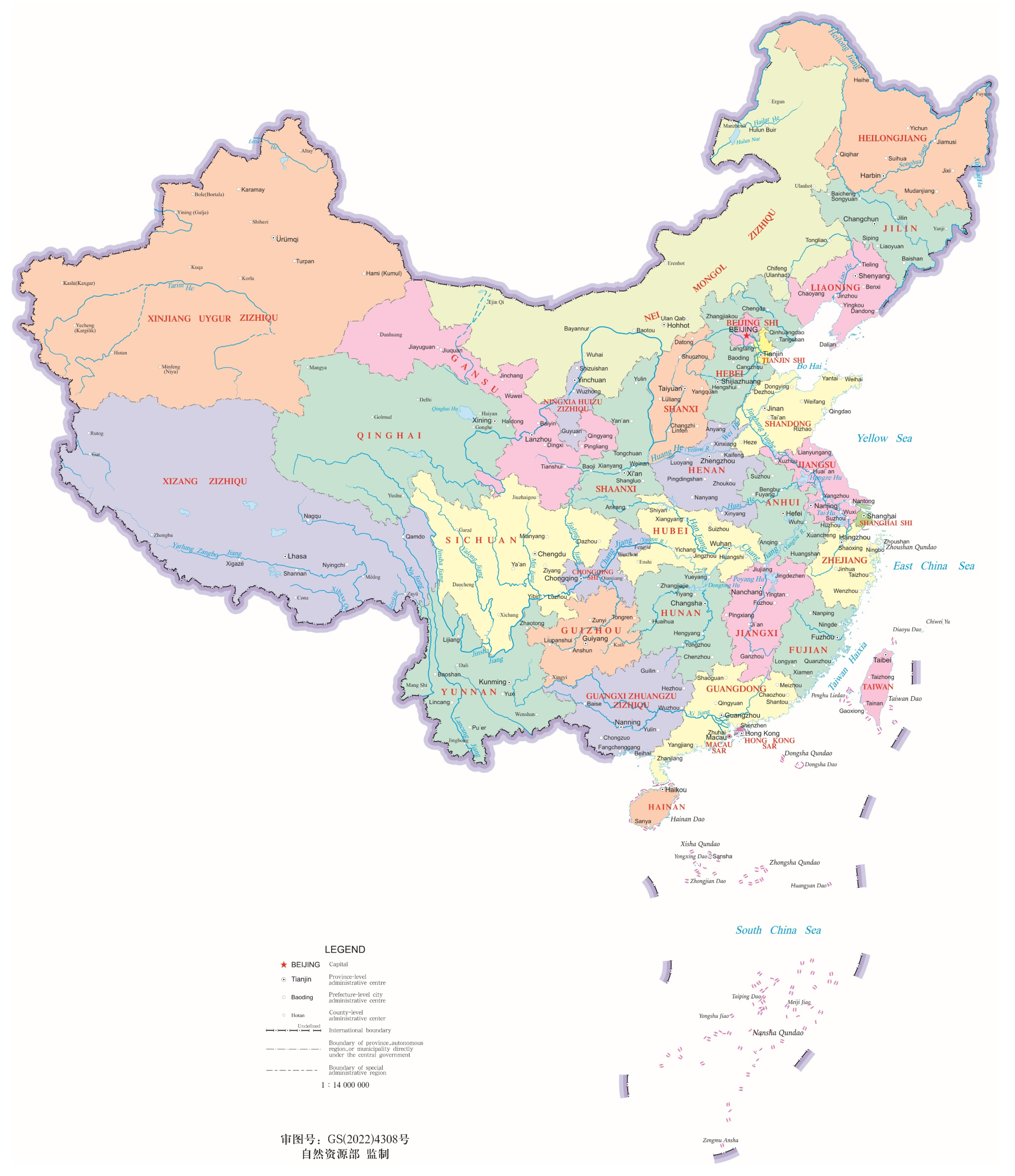
48]. Nevertheless, the innovation stratum, which is situated between the initial and secondary thresholds, may have reaped most of the benefits from prior adoptions, with only marginal benefits from subsequent innovations. The diminishing influence of innovation beyond the second threshold could be attributed to the law of diminishing marginal returns, which holds that increased innovation endeavors will result in diminishing income increases. This decreasing trend may be exacerbated by other production constraints that producers encounter, such as educational or labor constraints. The following regions, mostly located in eastern China, surpassed this secondary innovation threshold: Beijing, Tianjin, Shanghai, Jiangsu, Zhejiang, Anhui, Shandong, Henan, Hubei, Guangdong, and Chongqing.
In the context of rural human capital, the coefficient 0.217, which delineated the influence of agricultural science and technological innovation on the development of agricultural-household income, maintained significance at the 1% level for values below the threshold of 8.0900. It is intriguing that this coefficient increased to 0.351 when rural human capital surpassed this threshold, indicating a more significant effect. This impact coefficient was significantly increased to 0.538 as rural human capital continued to increase beyond the 10.5400 threshold. This progression demonstrates a critical correlation: the bolstering effect of agricultural science and technological innovation on farm-household income increases as rural human capital improves. Guizhou, Yunnan, Gansu, Qinghai, Ningxia, Xinjiang, Jilin, Heilongjiang, Anhui, and Sichuan were among the central and western provinces identified as having yet to achieve the threshold for rural human capital as of the end of 2021. Only Beijing, Shanghai, and Guangdong had succeeded in surpassing the secondary rural human capital threshold.
The impact coefficient of ASTI on farm household income growth was 0.274 when the urban–rural population aging gap was below the threshold of 10.1000. This value increased to 0.391 as the gap surpassed the initial threshold, but it marginally decreased to 0.305 upon surpassing a more pronounced second threshold of 21.2000. This trend indicates that the impact of agricultural innovation on rural income increases during the early phases as the age gap between urban and rural areas widens; however, this increase tends to moderate after the second threshold is exceeded.
This dynamic arises as rural gains from agricultural technology may not be as apparent as they are in urban areas at smaller aging differentials. However, as this differential increases, rural sectors may increasingly rely on technology to increase agricultural productivity and, as a result, income, in response to potential labor deficits or other challenges induced via an aging population. However, at extreme age disparities, the inherent challenges become so pervasive that technological interventions alone are unable to address the labor and production shortfalls caused by an aging populace. The secondary aging threshold was exceeded in regions such as Beijing, Tianjin, Shanghai, Hebei, Zhejiang, Guangdong, and Chongqing by the end of 2021, with a substantial portion of the population residing in the eastern region of China.


