Article

Does Agricultural Science and Technological Innovation Always Boost Farmers’ Income? Evidence from China

by
Yi Xiang
,
Yuke Ding
and
Shaohua Yin
*
Business School, Central South University of Forestry and Technology of China, Changsha 410004, China
*
Author to whom correspondence should be addressed.
Agriculture 2024, 14(12), 2154; https://doi.org/10.3390/agriculture14122154
Submission received: 16 October 2024 / Revised: 17 November 2024 / Accepted: 17 November 2024 / Published: 27 November 2024
(This article belongs to the Section Agricultural Economics, Policies and Rural Management)

Abstract

:
Agricultural science and technological innovation (ASTI) provides important opportunities to enhance agricultural welfare. Based on comparative advantage, value chain, and resource dependence theories, this study employed a variety of econometric models, including fixed effects (FEs), panel-corrected standard errors (PCSEs), feasible generalized least squares (FGLSs), and the systematic generalized method of moments (SYS-GMM), to investigate the impacts of ASTI on farmers’ income using data from a panel of 31 Chinese provinces spanning from 2012 to 2021. Our results reveal that ASTI contributes significantly positively to income growth, but its effects are not uniform: the central and western regions benefit more from ASTI compared to the eastern region. Moreover, as the level of ASTI increases, its positive impact on income growth diminishes. However, regions with higher levels of rural human capital—measured by educational attainment and skills—experience a more pronounced amplification of ASTI’s benefits on income. Additionally, aging populations in both urban and rural areas initially enhance the influence of ASTI on farmers’ income, but this effect diminishes as demographic gaps widen.

1. Introduction

An increase in farmers’ income has profound significance in promoting rural economic prosperity and improving farmers’ living standards. With the rapid development of technology, agricultural technological innovation has become a key factor in promoting agricultural modernization and improving agricultural production efficiency. At present, agricultural development is facing an important stage of transition from traditional agriculture to modern agriculture, with tight resource constraints and increasing environmental pressure. There is an urgent need to solve development problems through technological innovation. This article studies the impact of agricultural technological development on farmers’ income, aiming to explore how to effectively promote increases in farmers’ income through technological innovation achievements and provide theoretical support and practical paths for achieving sustainable agricultural development and comprehensive rural revitalization.
Agriculture, as a cornerstone of global economies, is deeply intertwined with rural social stability and economic prosperity. However, challenges such as population growth, shrinking arable land, and climate change are pressuring traditional agricultural models, rendering them increasingly insufficient in meeting food and agricultural demands. Agricultural science and technological innovation (ASTI) has emerged as a key driver in improving agricultural productivity and increasing farmers’ incomes. This includes advancements and applications in a variety of fields, such as new planting techniques, high-yield crop varieties, digital agricultural tools, and agricultural mechanization [1,2]. For instance, the economic benefits for farmers have been enhanced with the adoption of precision agricultural technology in Europe, America, and countries in other regions, which has reduced production costs and increased crop yields. In addition, the Chinese government has established robust frameworks to stimulate the development of agricultural science and technology and increase the income of farmers.
However, there are still research gaps in the literature. On the one hand, there is a gap in the research on the relationship between ASTI and the incomes of farmers. Despite the wealth of studies on science, technology, and innovation (STI), there is limited research exploring the impact of ASTI on farmers’ benefits and how these impacts vary across different regions [3,4,5]. Of relevance to this are the significant differences in education, geography, and other endowments between different regions in some countries, which may lead to changes in the economic effects of ASTI. On the other hand, research on the dynamic effects of ASTI is also lacking. Previous studies have explored the long-term impact of technology and innovation. Such technologies may not assume an obvious role in the initial period of their adoption, depending on their recognition and popularization. Indeed, farmers may adopt ASTI later due to their perception of technology or their education level, resulting in a lag effect in the change in farmers’ income. Nonetheless, ASTI may have dynamic effects that are missed in long-term studies. Furthermore, there is also a research gap in the literature in terms of empirical studies on STI. Many studies have discussed the role and value of STI, but they mainly rely on qualitative analysis, lacking empirical research to provide adequate evidence [6,7,8].
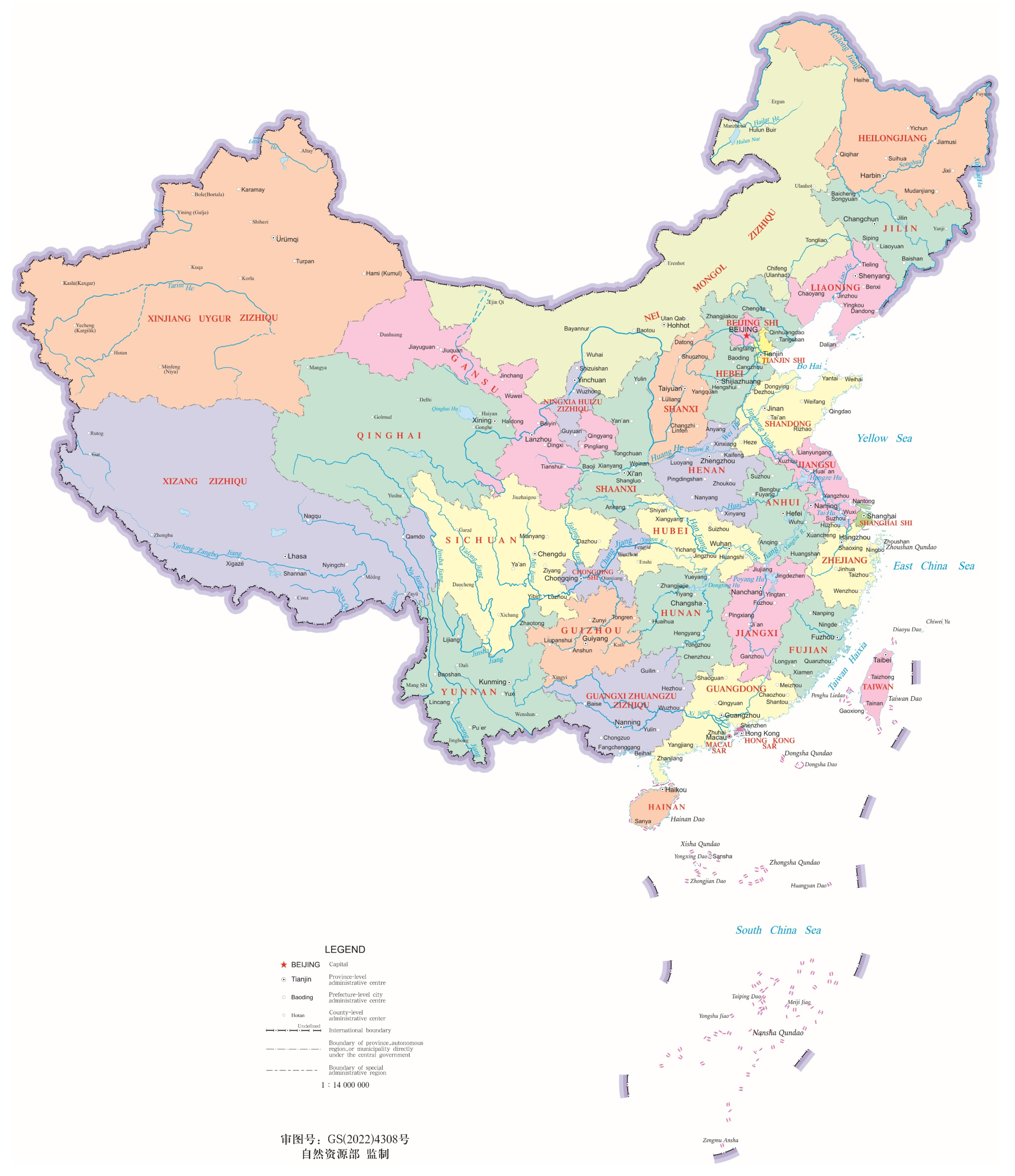
This study fills this research gap by focusing on regional disparities and examining how ASTI contributed to income growth across China’s eastern, central, and western provinces between 2012 and 2021 using advanced econometric models [9]. While science, technology, and innovation (STI) are widely recognized as key drivers of enhanced agricultural productivity and product quality, their benefits are not uniformly distributed. Existing studies have highlighted challenges such as financial barriers and access to specialized training [10,11]. This disparity can limit STI adoption, particularly for poorer farm households, exacerbating regional inequalities [12]. Previous research has largely focused on the overall impact of STI on agricultural output, while few studies have comprehensively explored its direct effects on household income, especially in regions with varying economic and technological capabilities. This study aims to bridge that gap by exploring how ASTI impacts farmers’ incomes across different regions in China. As shown in Figure 1, there are significant geographical differences among the eastern, central, and western regions of China. The eastern region has flat terrain, dense rivers, large amounts of precipitation, and a developed economy, so its agricultural endowment is relatively rich. The central and western regions are mainly mountainous and hilly, with sparse rivers, so the agricultural endowment is relatively poor. There may be significant differences between these regions in terms of the effectiveness of applying ASTI.
Additionally, the integration of STI could inadvertently exacerbate existing inequalities by granting only a privileged subset of the farming community unrestricted access and proficiency in assimilating these technological advancements [12]. Consequently, a dichotomy arises: while STI has the potential to significantly increase agricultural output, its financial implications and inherent disparities may limit the potential for income growth for a portion of the farming population.
This study also fills the gap in the study of the dynamic effects of STI. Several studies have investigated the effects of STI on broad agricultural economic dynamics, but there is an absence of literature that comprehensively examines the correlations between ASTI and income augmentation for farm households [13]. A nuanced, bidirectional relationship between ASTI and the economic well-being of the agricultural sector has been revealed through empirical studies [14]. Regions that are at the forefront of cutting-edge STI consistently exhibit superior agricultural economic trajectories. These insights invariably raise the question of whether a thriving agricultural economy unambiguously indicates a corresponding increase in farmers’ income. To answer that question, we examined the dynamic effect of ASTI, which reflects the lagging impact of urban and rural disparities such as population aging and human capital on the relationship between ASTI and the incomes of farmers.
This study provides a large amount of empirical evidence to fill the quantitative research gap on STI. We incorporated macroeconomic panel data from various Chinese provinces covering the period from 2012 to 2021, and we developed both static and dynamic panel analytical frameworks using a composite index that measures competency in ASTI and its effect on farm household income. Various analytical methodologies, such as fixed effects (FEs), panel-corrected standard errors (PCSEs), feasible generalized least squares (FGLSs), and systematic moment estimation (SYS-GMM), were employed to examine the influence of ASTI on the incomes of farming households. The analysis specifically focused on regional disparities and utilized panel threshold models.
The remaining structure of this paper is as follows: Section 2 discusses our theoretical analysis and research hypothesis, Section 3 presents the materials and methods, Section 4 outlines the empirical tests performed and our analysis of results, and Section 5 and Section 6 present a discussion and a conclusion, respectively.

2. Theoretical Analysis and Research Hypothesis

2.1. Mechanism Underlying How ASTI Impacts the Increase in Farmers’ Income

In income growth theory, the core assumption is that ASTI is the intrinsic driving force behind an income increase [15,16]. In the field of agriculture, ASTI involves a combination of the land, the labor force, and technology (such as novel crop varieties and advanced agricultural methods) [17,18,19]. Technological advancements raise the overall production with the same amount of land and labor input [20], which leads to a cost reduction and increased productivity. Moreover, farmers can increase their production by embracing innovative technologies that concentrate their work on specialized agricultural pursuits [21]. Beyond those, further technological innovations have not only enhanced the amount and standard of farmers’ outputs but also decreased the amount of manual effort required [22,23]. Additionally, ASTI plays a vital role in enhancing market access, offers valuable insights that help farmers increase their sales networks, and ensures that they set advantageous pricing [24].
In such ways, ASTI has enabled farmers to increase their production of high-value-added and distinct products. For instance, there has been a constant increase in customer demand for organic food, pesticide-residue-free products, and items a region is known for [25], and ASTI—for instance, using precise fertilizer applications and pest management procedures—has empowered farmers to fulfill the requirements of these markets and consequently achieve elevated price premiums [26,27]. Moreover, farmers frequently encounter difficulties in comprehending market dynamics with precision because of constraints on the available information. By implementing technologies like the Internet of Things (IoT), big data, and artificial intelligence in agriculture, farmers may obtain up-to-date information on market prices, weather forecasts, and supply and demand [28,29,30]. Drawing on value chain theory reveals how ASTI may also optimize the value generated at each stage of production, including raw material selection, processing, and marketing, through technological intervention [31]. Technological improvements in agriculture may also enable farmers to create customized products for certain consumer segments, based on market segmentation. In the example from earlier of items that are free from pesticide residue or have organic certification, it is important for farmers to identify whether there is a consumer segment for these, as they generally command higher prices in the market [32,33,34].
Hypothesis 1 (H1):
ASTI enhances farmers’ income by improving production efficiency, expanding market demand, and raising product value.

2.2. The Impact of ASTI on Farmers’ Income Is Regionally Heterogeneous

Both Reed’s law and Metcalfe’s law suggest that networks display significant externalities and positive feedback effects. ASTI is an externality that may be deeply integrated into the network of agricultural production via advanced information technology. The value of ASTI for raising farmers’ income will increase significantly if the size of the network exceeds a certain threshold. Unlike other systems, ASTI’s positive feedback mechanism is only triggered if a specific level of maturity is reached. This implies that continuing improvements in ASTI might lead to the exponential development of its advantages and increase farmers’ revenue. There are several reasons for this, which are as follows.
Initially, ASTI undergoes significant and progressive changes over a launch period [35,36,37]. Disparities in the level and use of ASTI among areas are influenced by regional climate variability, soil conditions, agricultural policies, and technology uptake. However, once ASTI in a specific region surpasses a particular level, it can significantly enhance the favorable effect on farmers’ income. Furthermore, the extensive data and valuable insights collected via ASTI can be optimized through economies of scale when implemented at the local level. Once ASTI reaches a certain threshold, the expenses incurred by farmers to obtain new technology, market data, and other resources decrease considerably. Therefore, the beneficial influence of innovation on farmers’ income shows a slightly upward trajectory. Ultimately, the inherent risks associated with ASTI, such as reliance on technology and ecological imbalances, may initially impede farmers’ income increase; however, as ASTI develops, the influence of these risks decreases, consequently enhancing the positive effect of this innovation on the incomes of farm households.
Hypothesis 2 (H2):
Due to regional differences in terrain and the geographical environment, there is a lack of agricultural technological implementation, which, in turn, affects farmers’ income growth.

2.3. Dynamic Threshold Effect Analysis of ASTI Driving Farmers’ Income Increase

Both Reed’s law and Metcalfe’s law suggest that networks display significant externalities and positive feedback effects. ASTI is an externality that may be deeply integrated into the network of agricultural production via advanced information technology. The value of ASTI for raising farmers’ income will increase significantly if the size of the network exceeds a certain threshold. Unlike other systems, ASTI’s positive feedback mechanism is only triggered if a specific level of maturity is reached. This implies that continuing improvements in ASTI might lead to exponential development of its advantages and increase farmers’ revenue. There are several reasons for this, which are as follows.
Initially, ASTI undergoes significant and progressive changes over a launch period. Disparities in the level and use of ASTI among areas are influenced by regional climate variability, soil conditions, agricultural policies, and technology uptake. However, once ASTI in a specific region surpasses a particular level, it can significantly enhance the favorable effect on farmers’ income. Furthermore, the extensive data and valuable insights collected via ASTI can be optimized through economies of scale when implemented at the local level. Once ASTI reaches a certain threshold, the expenses incurred by farmers to obtain new technology, market data, and other resources decrease considerably. Therefore, the beneficial influence of innovation on farmers’ income shows a slightly upward trajectory. Ultimately, the inherent risks associated with ASTI, such as reliance on technology and ecological imbalances, may initially impede farmers’ income increase; however, as ASTI develops, the influence of these risks decreases, consequently enhancing the positive effect of this innovation on the incomes of farm households.
Hypothesis 3 (H3):
The effects of ASTI on farmers’ income diminish progressively as ASTI levels increase.
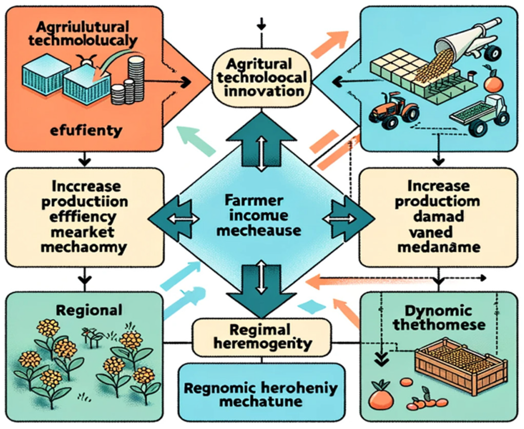
The direct relationship between the increase in producers’ income and ASTI is demonstrated by the theoretical analysis framework in Figure 2. ASTI enhances producers’ income via three primary mechanisms: Initially, it enhances production efficiency and allows producers to produce a greater quantity of high-quality agricultural products on fixed land. Secondly, it assists producers in meeting the high-value demand of specific markets, expands market demand, and adjusts production strategies in real time. Finally, it increases the market value of producers and improves the added value of products. However, the extent to which farmers in various regions may benefit from technological advancements may vary due to resource variations, technical acceptability, and geographic location. Furthermore, the development and widespread application of technology may result in a significant increase in farmers’ incomes; however, this effect may ultimately diminish.

3. Materials and Methods

3.1. Data Sources

This study analyzed panel data collected from 31 provinces spanning the years 2012 to 2021. To enhance the robustness of our analysis, we managed occasional missing values and outliers using advanced smoothing and interpolation techniques. We collected relevant datasets by obtaining comprehensive records from reputable publications such as the China Statistical Yearbook, China Agricultural Yearbook, China Science and Technology Statistical Yearbook, China County Statistical Yearbook, China Rural Statistical Yearbook, and China Employment and Population Yearbook. In addition, we integrated data from the EPS database, provincial statistics yearbooks, and relevant policy documents released by the Ministry of Agriculture and Rural Development. The above data sources are all from the Chinese government (National Bureau of Statistics of China: https://www.stats.gov.cn/sj/ndsj/). Due to statistical limitations, data on ASTI, such as agricultural patent applications, authorizations, total counts of agricultural scientific publications, and the number of full-time equivalent employees for agricultural R&D professionals, were not available prior to 2012. Furthermore, most of the relevant datasets collected after 2021 have not yet been made available to the public; consequently, this study’s temporal scope was set from 2012 to 2021.

3.2. Selection and Measurement of Variables

(1)
The outcome variable was the income of farmers
The income of farmers was measured by the per capita disposable income of rural residents, expressed in units of RMB 10,000 (USD 1 ≈ RMB 7.179, based on 2023.12).
(2)
The independent variable was the level of ASTI
ASTI is a complex process rooted in a particular agricultural scientific and technological environment, with the goal of introducing and promoting new varieties and methods of agricultural production, thereby ensuring a balanced integration of economic, social, and ecological elements. This complex process is principally supported by four fundamental elements:
First, the ASTI environment serves as the foundation for agricultural innovation efforts, highlighting the importance of the main contributors to agricultural innovation within the larger socio-economic context. Second, tangible infrastructure and resources are provided for agricultural innovation activities, which are particularly crucial for the development of new products.
Third, many resources and much capital are utilized in scientific and technical agricultural activities, which contribute to the development of new knowledge, technologies, and outcomes. The need for a sound distribution and integration of resources for innovation is crucial to consider. Fourth, the results of the innovation and the resulting increase in value act as prominent measures to assess the success of any inventive endeavor.
This index framework is shown in Table 1. According to the impact of the change in each index value, we calculated the entropy and determined the overall weight of that index. Furthermore, the level of ASTI was acquired by multiplying the weight by the real value (after normalization) of each index. The computation proceeded as follows:
P i j = [ p i j p min ( j ) ] / [ p max ( j ) p min ( j ) ]
Formula (1) is the process of normalization for each index. i indicates the province, and j indicates the index. p i j is the value of index j for province i . p min ( j ) and p max ( j ) are the min and max for index j . P i j is the value of index j in province i after normalization, which ranges from 0 to 1.
Furthermore, we need to calculate the entropy of each indicator. The calculation formula of information entropy is as follows:
H j = k i = 1 n P i j l n ( P i j )
In Formula (2), H j is the information entropy of index j , which means that the greater the uncertainty of information, the greater the entropy and the more information it contains. k is a normalization constant, which equals 1 / l n ( n ) in general, and n is the number of provinces.
Then, information entropy redundancy should be calculated to identify the extent of valid information.
D j = 1 H j
In Formula (3), D j is the information entropy redundancy of index j . Based on this, we can acquire the weight of each indicator. The equation is as follows:
W j = D j j = 1 m D j
In Equation (4), W j is the weight of index j , and D j is the information entropy redundancy of index j .
Finally, we can calculate the scores of each index to horizontally compare the rankings of the indexes:
M i = j = 1 n W j P i j
where M i is the composite ASTI index for province i , and the higher the value of M i , the higher the level of ASTI, while W j is the weight of index j .
(3)
Control variables
To improve the robustness of our study, we included several control factors in this analysis, including fiscal support for agriculture, rural human capital, the urban registered unemployment rate, and the urban–rural population age disparity (Table 2).
Fiscal support for agriculture: This metric represents the proportion of local agricultural fiscal allocations relative to the total local fiscal disbursements, expressed as a percentage.
Rural human capital: This parameter is expressed in years, quantifying the mean duration of education received by farmers across various provinces and districts. Using data from the China Rural Statistical Yearbook, the literacy-level stratification of the rural household workforce was categorized into six distinct brackets:
  • Illiterate or merely literate: corresponding to 1 year of formal education.
  • Primary school: corresponding to 6 years.
  • Junior high school: corresponding to 9 years.
  • Senior high school and secondary school: corresponding to 12 years.
  • Post-secondary school and beyond: corresponding to 16 years.
Urban registered unemployment rate: This denotes the documented unemployment proportion in urban areas, expressed as a percentage.
Urban–rural population age disparity: This metric is measured as the ratio between the urban and rural old-age dependency ratios.

3.3. Model Setting and Estimation Methods

This study aimed to analyze the impact of ASTI on farmers’ incomes and regional disparities. It drew upon multiple regressions outlined in the academic literature that examined the factors influencing agricultural economic growth [38,39,40,41]. The method of multiple regression analysis was utilized in the aim of exploring the relationship between ASTI and farmers’ incomes while keeping other factors constant. We developed the following econometric framework:
INC i t = α 0 + α 1 INN i t + μ i + ε i t
In Formula (6), i and t indicate the province and year, respectively. Variables INC i t and INN i t correspond to the magnitude of farm household income and the level of ASTI, respectively. The coefficient α 1 was of interest to us, which represents the impact of ASTI on the agricultural incomes of farmers. μ i captures the unobserved regional effects, and ε i t is the stochastic error term.
Beyond the scope of ASTI, the income dynamics of farm households are influenced by a variety of factors, including demographic aging, the prevailing unemployment landscape, the shortage of rural human capital, and fiscal patronage. To ensure that our model was comprehensive, we incorporated these variables in a modified Equation (6), as illustrated in the following:
INC i t = α 0 + α 1 INN i t + α 2 FIN i t + α 3 EDU i t + α 4 UNE i t + α 5 A G E i t + μ i + ε i t
In Formula (7), FIN i t is the financial support for agriculture; EDU i t is the rural human capital; UNE i t is the urban registered unemployment rate; and A G E i t is urban–rural population aging. In acknowledging the potential estimation biases introduced by omitted variables and considering that farm household income-generation efficiency may be historically contingent, this analysis introduced a first-order lag term of the explanatory variable—specifically, the agricultural scientific and technological innovation. Hence, we built the dynamic panel model below:
I N C i t = β 0 + β 1 I N C i , t 1 + β 2 I N N i t + β 3 F I N i t + β 4 E D U i t + β 5 U N E i t + β 6 A G E i t + μ i + ε i t
In this formula, I N C i , t 1 captures the farm household income metric from the previous period. The coefficient β 1 reflects that the dynamic effect of ASTI, which includes the impact of the level of ASTI in the previous year on the current period. This formula seeks to amalgamate historic data points with present indicators, fostering a comprehensive analysis.
Formulas (6) and (7) aim to explore the impact of ADSI on farmers’ income, and (8) further explores the dynamic effect of ASTI. When choosing static panel data, we used a systematic approach whereby we performed the F, LM, and Hausman tests [42]. Afterwards, we conducted tests specifically designed to detect heteroskedasticity and autocorrelation in the static panel data structure. The above methods mainly identify the stationarity of the model [43,44].
In general, multiple regressions are combined with fixed-effects models. When the panel-estimating model is affected by heteroskedasticity or autocorrelation, the PCSE (panel-corrected standard error) and FGLS (feasible generalized least square) approaches are considered appropriate alternatives for re-estimation. To explore the dynamic effect of ASTI, we used the SYS-GMM (systematic generalized method of moments) technique as the preferred estimator for our analysis, specifically focusing on dynamic panel data handling.

4. Empirical Tests and Analysis of Results

4.1. Analysis of Baseline Test Results

First, we addressed potential multicollinearity in the static panel model. The results of our diagnostic study showed that the mean variance inflation factor (VIF) was 1.39, and the maximum VIF for any explanatory variable was 1.67. Both values met the conventional criterion of 5, which meant that we did not find considerable multicollinearity among the variables in our model.
Next, using the static panel analysis framework, we performed the critical task of selecting the model configuration. Random effects (REs), fixed effects (FEs), and pooled ordinary least squares (POLSs) were the candidate models evaluated, which represent alternative methods for evaluating the economic effect [45]. They can be used to explore the same research question, only differing in their methods based on Equation (7). These models were thoroughly assessed using the F, LM, and Hausman tests, and the results indicated that the null hypotheses could be unanimously rejected at a 1% significance level. The FE (fixed-effects) method appeared the most appropriate for model estimation, as demonstrated by the results of the three tests.
We assessed the heteroskedasticity and autocorrelation of this FE model using the Wald and Wooldridge tests, respectively. The initial hypotheses were decisively rejected by the results, which yielded a p-value of 0.0000. This suggested that our model contained significant heteroskedasticity and autocorrelation. The model was recalibrated using both the PCSE and FGLS approaches in response.
Next, we assessed the dynamic panel model using the SYS-GMM estimation technique, and a breakdown of the estimative outcomes is given in Table 3.
As shown in Table 3, the impact of ASTI (Inn) on the growth of farmers’ incomes remained positive across models (1) to (4). The coefficient of Inn was significant at the 1% level. The results in column (3) indicate that, for every unit increase in the level of ASTI, farmers’ income will increase by 0.689. This discovery is consistent with actual trends, that is, the upward trajectory of China’s agricultural innovation and its synergistic positive impact on the incomes of farmers.
Table 3 also illustrates that the robustness levels of the fit for models (1) and (2) were 0.835 and 0.651, respectively. These results validated the model’s overall accuracy. The Wald statistic of model (3), which was developed using the FGLS technique, was validated at the 1% significance level, affirming the model’s structural integrity and result reliability. Furthermore, through the SYS-GMM approach, we found that the AR (2) test did not identify secondary serial autocorrelation in first-order differentiated residuals when applied to model (4). Additionally, the Hansen test yielded a p-value that exceeded 0.1, which substantiated the rationale for the dynamic panel model and validated our instrumental variable selection.
With a further investigation of auxiliary control variables, we discovered that agricultural financial support (Fin) had a detrimental effect on the development of farmers’ incomes. This may be attributed to the suppression of innovation uptake as a result of subsidies for using traditional farming methods. The correlation between human capital (Edu) and farm income demonstrated a robust positive trend, underscoring the importance of improved education in facilitating the integration of agricultural technology and increasing productivity. Farm income was adversely affected by the urban unemployment metric (Une), which can be attributed to factors such as reduced urban job opportunities and suppressed agricultural demand. Furthermore, the urban–rural age disparity (Age) positively impacted farm income, likely because of the dynamism of a youthful rural workforce and age-related policy favoritism.
Finally, when lagged ASTI effects were considered, a strong correlation was observed between the farm income growth of the previous year (L. Inc) and its current-year counterpart (Inc). This finding emphasizes the cumulative, enduring nature of income growth, as present earnings closely resemble past financial trajectories.

4.2. Analysis of the Results of the Regional Differences Test

A comprehensive analysis of the regional variations in the impact of ASTI on the economic situation of farm households is provided in Table 4. Models (1) to (3) concentrate on the eastern region, while models (4) to (6) provide insights into the central and western regional samples. The robustness of our model framework was ensured through the integration of R2 values, Wald’s statistics, the AR (2) test, and Hansen’s test results, which guaranteed the accuracy of our assessments and the suitability of our instrumental variable selection for the context.
The eastern region’s agricultural science and technological innovation (Inn) coefficients were 0.665, 0.665, and 0.078, respectively, at a 1% significance threshold, as revealed by an examination of the core explanatory variable metrics. Meanwhile, the central and western region’s coefficients were 0.808, 0.808, and 0.095 at the 1% significance level. These discrepancies emphasize the regional variations in the way agricultural innovations influence the income trajectories of farm households. It is intriguing that the central and western provinces have experienced a more significant increase in farm household incomes because of these innovations than their eastern counterparts. This distinction aligns with our second hypothesis (H2) and reinforces its validity.

4.3. Robustness Tests

To enhance the rigor of our preliminary tests, we sought to ensure the findings’ validity by reviewing the quantification procedure for the markers that depicted the level of ASTI. Here, principal component analysis was utilized to adjust the weights of innovation’s secondary indicators, instead of the entropy method previously used. As a result, a new composite index called “Inns” was created at the ASTI level. Later, we implemented a modification by replacing the variable for the rise in income of farm households [46]. More precisely, the initial independent variable representing the disposable income of farmers was replaced with a measurement indicating the disposable income of rural households.
Table 5 displays the outcomes of these rigorous assessments. An important observation that can be made is that the uniformity of the estimates for the fundamental explanatory variable (Inn) at all levels. Although there is a small variation in magnitude, the direction and statistical significance remain constant at both the national and sub-regional levels. This coherence undeniably strengthens our initial conclusions, confirming their trustworthiness. The analysis suggested that ASTI had a substantial impact on the increase in agricultural household income, but with significant regional disparities. We conducted additional research to identify the prospective factors contributing to these regional disparities.

4.4. Analysis of Factors Affecting Regional Disparities

Our empirical analysis suggested that agricultural innovations substantially impacted the increase in farms’ incomes. Nevertheless, the advantages derived from innovation-driven income varied due to the significant variation in the innovation landscape across different regions. Additionally, the adoption and implementation of new agricultural methods can be facilitated through the enhancement of rural human capital, which, in turn, leads to an increase in the income of farm households. It was thus plausible to anticipate that regions with robust rural human capital would be more receptive to the favorable financial consequences of innovations. Additionally, we determined that the considerable age disparities between urban and rural populations contribute to the increase in farm household incomes by prompting the migration of rural labor to urban employment, following which those laborers supplement rural incomes through money sent back from their non-agricultural activities. A favorable environment for the promotion of agricultural innovation and dynamism was suggested in the trends of urbanization and a relatively youthful rural population. In general, younger generations are more adept at utilizing new agricultural technologies and are more receptive to them. As a result, regions with substantial disparities in urban–rural aging are well positioned to capitalize on the potential of agricultural innovations to increase the incomes of farm households.
Regional heterogeneity in the financial benefits of agricultural innovations was found to be influenced by factors such as the urban–rural demographic disparity and rural human capital. This implied the existence of prospective “threshold characteristics” in relation to the impact of these innovations on the incomes of farm households. In other words, the impact of these innovations had discernible variations contingent upon distinct thresholds associated with the level of innovation, rural human capital, and urban–rural age disparities. To elucidate this further, our research team created a panel threshold model that investigated the threshold-centric attributes of agricultural innovation’s impact on farm household income. This model was predicated on regional factors, including the level of agricultural innovation, rural human capital, and urban–rural aging differentials.
(1)
Model and Estimation Method
We modified Hansen’s analytical paradigm to identify the non-linear threshold association between agricultural innovation and an increase in farm family income to investigate the heterogeneity of the effect of ASTI in raising farm household income [44,47]. In this way, we developed three-panel threshold models derived from the basic econometric model (7). The basic idea of this model is to estimate the possible inflection point values and then perform tests to obtain the corresponding confidence intervals. Our models used the following threshold determinants: the urban–rural population age divergence (Age), rural human capital (Edu), and agricultural science and technological innovation (Inn). Agricultural scientific and technological innovation (Inn) was studied as the dependent variable of interest in these thresholds.
Inc it = a 0 + a 1 Inn it I ( Inn it γ 1 ) + a 2 Inn it I ( γ 1 < Inn it γ 2 ) + + a n Inn it I ( γ n 1 < Inn it γ n ) + a n + 1 Inn it I ( Inn it > γ n ) + λ C o n t r o l i t + μ i + ε i t
Inc it = β 0 + β 1 Inn it I ( Edu it ν 1 ) + β 2 Inn it I ( ν 1 < Edu it ν 2 ) + + β n Inn it I ( ν n 1 < Edu it ν n ) + β n + 1 Inn it I ( Edu n > ν n ) + ϕ C o n t r o l i t + μ i + ε i t
I n c i t = δ 0 + δ 1 I n n i t I ( A g e i t σ 1 ) + δ 2 I n n i t I ( σ 1 < A g e i t σ 2 ) + + δ n I n n i t I ( σ n 1 < A g e i t σ n ) + δ n + 1 I n n i t I ( A g e i t > σ n ) + θ C o n t r o l i t + μ i + ε i t
The models considered different thresholds based on the level of education, the age of rural residents, and the age disparity between urban and rural areas. In Formulas (9)–(11), γ n , ν n , and σ n represent the thresholds at different levels. The model segments the data based on these values to explore the influence of Innit within these segments. a 1 a n + 1 , β 1 β n + 1 , and δ 1 δ n + 1 depict how ASTI affects a farm’s income within the intervals defined by the thresholds γ n , ν n , and σ n . A significant difference between them would emphasize the importance of the selected threshold variables. μ i are fixed effects specific to each province, capturing any province-specific characteristics that do not change over time. E i t represents random error terms, accounting for unobserved factors affecting the dependent variable.
(2)
Threshold effect test
Prior to examining the specifics of the threshold model, we initially determined the threshold values, which are shown in Table 6. The data indicated the presence of two clear threshold values for agricultural science and technological innovation (Inn) at 0.6603 and 0.8747. Regarding rural human capital (Edu), the minimum value was 8.0900, and the maximum value was 10.5400. As for the urban–rural population age disparity (Age), the minimum value was 10.1000, and the maximum value was 21.2000. All of these values fell inside the corresponding 95% confidence intervals, which strongly indicated that our threshold calculations were based on solid evidence.
(3)
Estimation of threshold parameters
The estimations of the threshold model are delineated in Table 7, and they were obtained via a comprehensive threshold effect analysis. This analysis considered variables such as the urban–rural population age disparity (Age), rural human capital (Edu), and agricultural science and technological innovation (Inn). A careful examination of the table reveals that the impact coefficient of Inn on the growth of farm household income is a robust 0.474, which is significant at the 1% level, when agricultural innovation levels are below the 0.6603 threshold. Although this coefficient remains positively significant, it experiences a slight decline to 0.376 as innovation levels fluctuate between the first and second thresholds. The coefficient undergoes an additional decrease to 0.284 upon surpassing the second threshold, which is set to 0.8747. This progression emphasizes the complexity of the relationship. Initially, the introduction of innovative agricultural practices, including new seed variants, fertilizers, and improved irrigation systems, results in a significant increase in productivity and, as a result, substantial income growth [48]. Nevertheless, the innovation stratum, which is situated between the initial and secondary thresholds, may have reaped most of the benefits from prior adoptions, with only marginal benefits from subsequent innovations. The diminishing influence of innovation beyond the second threshold could be attributed to the law of diminishing marginal returns, which holds that increased innovation endeavors will result in diminishing income increases. This decreasing trend may be exacerbated by other production constraints that producers encounter, such as educational or labor constraints. The following regions, mostly located in eastern China, surpassed this secondary innovation threshold: Beijing, Tianjin, Shanghai, Jiangsu, Zhejiang, Anhui, Shandong, Henan, Hubei, Guangdong, and Chongqing.
In the context of rural human capital, the coefficient 0.217, which delineated the influence of agricultural science and technological innovation on the development of agricultural-household income, maintained significance at the 1% level for values below the threshold of 8.0900. It is intriguing that this coefficient increased to 0.351 when rural human capital surpassed this threshold, indicating a more significant effect. This impact coefficient was significantly increased to 0.538 as rural human capital continued to increase beyond the 10.5400 threshold. This progression demonstrates a critical correlation: the bolstering effect of agricultural science and technological innovation on farm-household income increases as rural human capital improves. Guizhou, Yunnan, Gansu, Qinghai, Ningxia, Xinjiang, Jilin, Heilongjiang, Anhui, and Sichuan were among the central and western provinces identified as having yet to achieve the threshold for rural human capital as of the end of 2021. Only Beijing, Shanghai, and Guangdong had succeeded in surpassing the secondary rural human capital threshold.
The impact coefficient of ASTI on farm household income growth was 0.274 when the urban–rural population aging gap was below the threshold of 10.1000. This value increased to 0.391 as the gap surpassed the initial threshold, but it marginally decreased to 0.305 upon surpassing a more pronounced second threshold of 21.2000. This trend indicates that the impact of agricultural innovation on rural income increases during the early phases as the age gap between urban and rural areas widens; however, this increase tends to moderate after the second threshold is exceeded.
This dynamic arises as rural gains from agricultural technology may not be as apparent as they are in urban areas at smaller aging differentials. However, as this differential increases, rural sectors may increasingly rely on technology to increase agricultural productivity and, as a result, income, in response to potential labor deficits or other challenges induced via an aging population. However, at extreme age disparities, the inherent challenges become so pervasive that technological interventions alone are unable to address the labor and production shortfalls caused by an aging populace. The secondary aging threshold was exceeded in regions such as Beijing, Tianjin, Shanghai, Hebei, Zhejiang, Guangdong, and Chongqing by the end of 2021, with a substantial portion of the population residing in the eastern region of China.
5. Discussion

This study has revealed significant regional differences in the impacts of ASTI on farmers’ incomes, especially in the central and western regions of China. That finding led us to consider the mechanisms behind regional differences. The existing research has confirmed the role of technological innovation in increasing farmers’ incomes, including via channels such as computer penetration, agricultural scale management, and e-commerce participation [47,49,50]. However, it has focused more on the overall effect and not considered regional differences. In other areas, numerous scholars have discussed the regional heterogeneity in China related to, for instance, energy efficiency [51], carbon emissions [52,53,54], technological innovation [55], and financial agglomeration [56,57]. Therefore, our paper filled a gap in exploring the regional heterogeneity of the impacts of ASTI on the incomes of farmers.
We further explored the influencing factors in regional heterogeneity. The existing literature mainly attributes urban–rural disparities to infrastructure and human capital [58,59] and to rural endowments negatively impacting rural areas. In regard to the imbalanced urban–rural development in China, this study highlights that population aging provides an opportunity for technological substitution to some extent, especially in the context of labor shortage. Here, automation and mechanization technologies may hold the key to making up for the labor gap. However, with the loss of the young labor force, an excessive dependence on technological substitution may lead to bottlenecks in the popularization and application of technology. Therefore, policies should address how to balance the labor shortage caused by aging with the promotion of scientific and technological innovation, especially for scientific and technological support in areas with serious labor loss.
Based on our findings, we can draw some policy implications: (1) Increase support for ASTI in the central and western regions. This research shows that agricultural science and technological innovation play a more significant role in increasing the incomes of farmers in the central and western regions. Therefore, policies should increase support for scientific and technological research and development and infrastructural construction in these areas, as well as promote the application of agricultural scientific and technological achievements in these areas. (2) Enhance rural human capital. The improvement of rural human capital can enhance the effect of ASTI. Therefore, policies should strengthen the skills training for the rural labor force, especially in modern ASTI, to help farmers better apply scientific and technological achievements and increase their income. (3) Optimize the impact of the age gap between urban and rural areas on STI. The change in the age gap between urban and rural populations will affect the impact of ASTI on income. Policies should focus on aging areas and ensure that all farmers benefit from technological innovation by providing employment opportunities and skill training. (4) Given the different effects of ASTI in different regions, policies should formulate differentiated support measures according to regional characteristics. Policies in the eastern region should focus on high-end agricultural science and technological research and development, while the policies in the central and western regions should strengthen the popularization of basic science and technology and promote the balanced growth of farmers’ incomes in various regions.

6. Conclusions

The findings suggest that ASTI universally functions as a catalyst for an increase in farm household income. Nevertheless, the effect of ASTI on income is intriguingly inconsistent across different regions. In comparison to their eastern counterparts, the central and western regions exhibit a more significant increase in income because of advancements in agricultural technology. The threshold benefit model was implemented to ascertain the underlying causes of these regional disparities. The insights obtained indicate that the positive effects of agricultural innovation on farm household income decrease as its magnitude increases. In contrast, the beneficial effects of these innovations on income are raised by an increase in rural human capital. Furthermore, initially, the positive impact of technological innovations on farm household income is raised by disparities in age demographics between urban and rural areas; however, the beneficial effects of innovation begin to diminish as these disparities become more pronounced over time.
However, note that, due to limitations in data availability and our research methods, we did include potential mechanisms such as farmers’ psychology and information technology uptake, which may require questionnaire surveys and rural experiments to explore. In some areas of China with strong traditional agricultural cultures, farmers may have a low acceptance of new technologies, which is not only a matter of their education level but also related to the farmers’ concept renewal and psychological adaptation. Accordingly, future research should address cultural factors and explore how to enhance farmers’ acceptance of new technologies through a combination of cultural adaptability and technology promotion to improve the effect of agricultural science and technological innovation. In addition, information technology may have an important impact on the incomes of farmers via precision agriculture and data-driven management, as well as by helping farmers better access the market and improve their price transparency and competitiveness. Therefore, we recommend that future research should focus on the application of information technology in agriculture and explore how it can promote agricultural modernization and improve farmers’ income levels through intelligent management.

Author Contributions

Conceptualization, S.Y.; Methodology, Y.D.; Data curation, Y.X. All authors have read and agreed to the published version of the manuscript.

Funding

This study was funded as a general project of National Social Science, “Research on Government Ecological Purchase Mechanism and Implementation Path Based on Green Development” (number: 19BJY045).

Institutional Review Board Statement

Not applicable.

Data Availability Statement

Data are contained within the article.

Conflicts of Interest

The authors declare no conflicts of interest.

References

  1. Islam, M.S.; Grönlund, Å. Bangladesh calling: Farmers’ technology use practices as a driver for development. Inf. Technol. Dev. 2011, 17, 95–111. [Google Scholar] [CrossRef]
  2. Neupane, D.; Adhikari, P.; Bhattarai, D.; Rana, B.; Ahmed, Z.; Sharma, U.; Adhikari, D. Does climate change affect the yield of the top three cereals and food security in the world? Earth 2022, 3, 45–71. [Google Scholar] [CrossRef]
  3. Dominguez Lacasa, I.; Molina Vogelsang, M. Enhancing international collaboration in science, technology, and innovation to achieve sustainable development goals. Sci. Public Policy 2024, 51, 509–525. [Google Scholar] [CrossRef]
  4. Saidi, T.; Douglas, T.S. Towards the socialization of science, technology and innovation for African development. Afr. J. Sci. Technol. Innov. Dev. 2018, 10, 110–113. [Google Scholar] [CrossRef]
  5. Webersik, C.; Wilson, C. Achieving environmental sustainability and growth in Africa: The role of science, technology and innovation. Sustain. Dev. 2009, 17, 400–413. [Google Scholar] [CrossRef]
  6. Manyuchi, A.E. Conceptualizing and institutions facilitating ‘use’ of innovation indicators in South Africa’s science, technology and innovation policymaking. Afr. J. Sci. Technol. Innov. Dev. 2018, 10, 483–492. [Google Scholar] [CrossRef]
  7. Dubeuf, J. Science, technology, innovation and governance for the goat sectors. Small Rumin. Res. 2014, 121, 2–6. [Google Scholar] [CrossRef]
  8. Hailu, G. Reflections on technological progress in the agri-food industry: Past, present, and future. Can. J. Agric. Econ. 2023, 71, 119–141. [Google Scholar] [CrossRef]
  9. Gao, Y.; Zang, L.; Sun, J. Does computer penetration increase farmers’ income? An empirical study from China. Telecommun. Policy 2018, 42, 345–360. [Google Scholar] [CrossRef]
  10. Zhang, Y. The regional disparity of influencing factors of technological innovation in China: Evidence from high-tech industry. Technol. Econ. Dev. Econ. 2021, 27, 811–832. [Google Scholar] [CrossRef]
  11. Wordofa, M.G.; Sassi, M. Impact of farmers’ training centres on household income: Evidence from propensity score matching in Eastern Ethiopia. Soc. Sci. 2017, 7, 4. [Google Scholar] [CrossRef]
  12. Liu, E.M. Time to change what to sow: Risk preferences and technology adoption decisions of cotton farmers in China. Rev. Econ. Stat. 2013, 95, 1386–1403. [Google Scholar] [CrossRef]
  13. Alston, J.M.; Pardey, P.G. Agriculture in the global economy. J. Econ. Perspect. 2014, 28, 121–146. [Google Scholar] [CrossRef]
  14. Huang, L.J.; Liu, L.Y.; Xiao, H.; Liu, X. Agricultural Science and Technology Innovation, Agricultural Technology Efficiency and Agricultural Economic Development—An Empirical Analysis Based on Vector Autoregressive (VAR) Model. Res. Sci. Technol. Manag. 2021, 41, 107–113. [Google Scholar]
  15. Tan, C.; Tao, J.; Yi, L.; He, J.; Huang, Q. Dynamic Relationship between Agricultural Technology Progress, Agricultural Insurance and Farmers’ Income. Agriculture 2022, 12, 1331. [Google Scholar] [CrossRef]
  16. Zhu, X.W. Exploration of the Way to Cross the Middle Income Trap Based on the Reality of Demographic Transition—The Perspective of Unified Growth Theory. J. Chongqing Univ. (Soc. Sci. Ed.) 2019, 25, 37–56. [Google Scholar]
  17. Welfens, P.J.J. Innovation, inequality and a golden rule for growth in an economy with Cobb-Douglas function and an R&D sector. Int. Econ. Econ. Policy 2015, 12, 469–496. [Google Scholar]
  18. DeLay, N.D.; Thompson, N.M.; Mintert, J.R. Precision agriculture technology adoption and technical efficiency. J. Agric. Econ. 2022, 73, 195–219. [Google Scholar] [CrossRef]
  19. Latruffe, L.; Bravo-Ureta, B.E.; Carpentier, A.; Desjeux, Y.; Moreira, V.H. Subsidies and technical efficiency in agriculture: Evidence from European dairy farms. Am. J. Agric. Econ. 2017, 99, 783–799. [Google Scholar] [CrossRef]
  20. Lv, C.Z.; Xu, L.Y. Measurement of total factor productivity in China’s agricultural production. Bus. Times 2012, 33, 132–133. [Google Scholar]
  21. Li, L.; Cai, K.; Li, Y. Mechanisms of e-commerce platform’s impact on agricultural business: Technological innovation drive and market channel widening. Rural Econ. 2021, 6, 120–128. [Google Scholar]
  22. Rao, E.J.O.; Brümmer, B.; Qaim, M. Farmer participation in supermarket channels, production technology, and efficiency: The case of vegetables in Kenya. Am. J. Agric. Econ. 2012, 94, 891–912. [Google Scholar] [CrossRef]
  23. Deng, F.; Jia, S.; Ye, M.; Li, Z. Coordinated development of high-quality agricultural transformation and technological innovation: A case study of main grain-producing areas, China. Environ. Sci. Pollut. Res. 2022, 29, 35150–35164. [Google Scholar] [CrossRef] [PubMed]
  24. Bhanot, D.; Kathuria, V.; Das, D. Can institutional innovations in agri-marketing channels alleviate distress selling? Evidence from India. World Dev. 2021, 137, 105202. [Google Scholar] [CrossRef]
  25. Huang, S.H.; Hu, X.P. Evaluation of Migrant Workers on Urban Public Cultural Products under the Perspective of Differentiated Demand. Financ. Sci. 2018, 5, 47–55. [Google Scholar]
  26. Porteous, O. Trade and agricultural technology adoption: Evidence from Africa. J. Dev. Econ. 2020, 144, 102440. [Google Scholar] [CrossRef]
  27. Zaman, K.; Khan, M.M.; Ahmad, M.; Rustam, R. The relationship between agricultural technology and energy demand in Pakistan. Energy Policy 2012, 44, 268–279. [Google Scholar] [CrossRef]
  28. He, Y.Q.; Xiong, Z.Y.; Zhang, K.; Wang, W. Digital economy development, non-farm employment and farmers’ income. Stat. Decis. Mak. 2023, 39, 111–115. [Google Scholar]
  29. Awada, L.; Phillips, P.W.B. Market power in smart farming and the distribution of gains in two-stage crop production system. J. Agric. Appl. Econ. Assoc. 2023, 2, 753–768. [Google Scholar] [CrossRef]
  30. Nicoletti, J.; Ning, C.; You, F. Incorporating agricultural waste-to-energy pathways into biomass product and process network through data-driven nonlinear adaptive robust optimization. Energy 2019, 180, 556–571. [Google Scholar] [CrossRef]
  31. Lou, X.Y.; Chen, S.Y.; Yang, L.W.; Li, M. An analysis of the competitiveness enhancement path of regional public brand of fruits in Shandong Province based on value chain theory. China Fruit Tree 2021, 8, 101–105. [Google Scholar]
  32. Liu, X.Y. Agricultural products intelligent marketing technology innovation in big data era. Procedia Comput. Sci. 2021, 183, 648–654. [Google Scholar] [CrossRef]
  33. Wang, C.; Zhang, L.; Chang, Y.; Pang, M. Biomass direct-fired power generation system in China: An integrated energy, GHG emissions, and economic evaluation for Salix. Energy Policy 2015, 84, 155–165. [Google Scholar] [CrossRef]
  34. Zhai, T.; Liu, J.; Wang, D. Optimization path of agricultural products marketing channel based on innovative industrial chain. Econ. Chang. Restruct. 2023, 56, 3949–3977. [Google Scholar] [CrossRef]
  35. Chen, Q. Advanced Econometrics and Stata Applications; Higher Education Press: Beijing, China, 2014. [Google Scholar]
  36. Ruttan, V.W. Induced innovation, evolutionary theory, and path dependence: Sources of technical change. Econ. J. 1997, 107, 1520–1529. [Google Scholar] [CrossRef]
  37. Lybbert, T.J.; Sumner, D.A. Agricultural technologies for climate change in developing countries: Policy options for innovation and technology diffusion. Food Policy 2012, 37, 114–123. [Google Scholar] [CrossRef]
  38. Luo, J.; Hu, J. Agricultural Credit Guarantee, Credit Supply, and Agricultural Economic Development: Empirical evidence from Chinese Interprovincial Panel Data. Res. Financ. Trade 2023, 1–14. [Google Scholar]
  39. Lian, J. Digital Financial Development, Rural Financial Inclusion, and Agricultural Economic Growth: Empirical evidence from Chinese County Data. China Soft Sci. 2022, 5, 134–146. [Google Scholar]
  40. Pang, J.; Yang, M. Rural Financial Development and Agricultural Economic Growth: Based on the Mediating Effect of Agricultural Science and Technology Innovation. Res. Sci. Technol. Manag. 2021, 41, 85–90. [Google Scholar]
  41. Dai, K.; Liu, Y. How factor market distortions affect innovation performance. World Econ. 2016, 39, 54–79. [Google Scholar]
  42. Hausman, J.; Stock, J.H.; Yogo, M. Asymptotic properties of the Hahn–Hausman test for weak instruments. Econ. Lett. 2005, 89, 333–342. [Google Scholar] [CrossRef]
  43. Lee, Y.; Okui, R. Hahn–Hausman test as a specification test. J. Econom. 2012, 167, 133–139. [Google Scholar] [CrossRef]
  44. Hansen, B.E. Threshold effects in non-dynamic panels: Estimation, testing, and inference. J. Econom. 1999, 93, 345–368. [Google Scholar] [CrossRef]
  45. Baltagi, B.H.; Bresson, G.; Pirotte, A. Fixed effects, random effects or Hausman–Taylor? A pretest estimator. Econ. Lett. 2003, 79, 361–369. [Google Scholar] [CrossRef]
  46. Liang, B.; Ji, H. How does unemployment insurance affect job search effort? Evidence from the China Time Use Survey. Econ. Res. 2020, 55, 179–197. [Google Scholar]
  47. Yi, F.; Yao, L.; Sun, Y.; Cai, Y. E-commerce participation, digital finance and farmers’ income. China Agric. Econ. Rev. 2023, 15, 833–852. [Google Scholar] [CrossRef]
  48. Sime, G.; Aune, J.B. Sustainability of improved crop varieties and agricultural practices: A case study in the central rift valley of Ethiopia. Agriculture 2018, 8, 177. [Google Scholar] [CrossRef]
  49. Yu, B. The impact of the internet on industrial green productivity: Evidence from china. Technol. Forecast. Soc. Chang. 2022, 177, 121527. [Google Scholar] [CrossRef]
  50. Yin, G.; You, Y.; Han, X.; Chen, D. The effect of agricultural scale management on farmers’ income from a dual-scale perspective: Evidence from rural China. Int. Rev. Econ. Financ. 2024, 94, 103372. [Google Scholar] [CrossRef]
  51. Yu, J.; Zhou, K.; Yang, S. Regional heterogeneity of China’s energy efficiency in “new normal”: A meta-frontier super-SBM analysis. Energy Policy 2019, 134, 110941. [Google Scholar] [CrossRef]
  52. Han, J.; Qu, J.; Maraseni, T.N.; Zeng, J.; Wang, D.; Ge, Y.; Wu, D. Spatiotemporal analysis of the food-related carbon emissions of China: Regional heterogeneity and the urban-rural divide. J. Environ. Manag. 2024, 370, 122441. [Google Scholar] [CrossRef] [PubMed]
  53. Liu, Q.; Ding, G.; Shu, K. Economic policy uncertainty, firm carbon emissions, and regional heterogeneity: Evidence from China’s exporters. Ann. Reg. Sci. 2024, 73, 521–555. [Google Scholar] [CrossRef]
  54. Yan, B.; Yan, X.; Jiang, X. Carbon productivity and value-added generations: Regional heterogeneity along global value chain. Struct. Chang. Econ. Dyn. 2023, 65, 111–125. [Google Scholar] [CrossRef]
  55. Che, X.; Zhou, P.; Wang, M. The policy effect on photovoltaic technology innovation with regional heterogeneity in China. Energy Econ. 2022, 115, 106385. [Google Scholar] [CrossRef]
  56. Xie, R.; Fu, W.; Yao, S.; Zhang, Q. Effects of financial agglomeration on green total factor productivity in Chinese cities: Insights from an empirical spatial Durbin model. Energy Econ. 2021, 101, 105449. [Google Scholar] [CrossRef]
  57. Dong, X.; Cui, R.; Bai, X.; Liu, K. Can digital inclusive finance reduce household poverty? Evidence from the China Household Finance Survey. Int. Rev. Econ. Financ. 2024, 96, 103603. [Google Scholar] [CrossRef]
  58. Yu, G.; Lu, Z. Rural credit input, labor transfer and urban–rural income gap: Evidence from China. China Agric. Econ. Rev. 2021, 13, 872–893. [Google Scholar] [CrossRef]
  59. Lu, H.; Zhao, P.; Hu, H.; Zeng, L.; Wu, K.S.; Lv, D. Transport infrastructure and urban-rural income disparity: A municipal-level analysis in China. J. Transp. Geogr. 2022, 99, 103292. [Google Scholar] [CrossRef]
Figure 1. Geographical differences in China. Source: Ministry of Natural Resources of the People’s Republic of China (2022). The content of non-English means No. GS (2024) 4308 of drawing number, supervised by the Ministry of Natural Resources.
Agriculture 14 02154 g001
Figure 2. Theoretical framework diagram of this study.
Agriculture 14 02154 g002
Table 1. Agricultural science, technology, and innovation indicator system.
Measurement IndexCodingVariable DefinitionOrientation
Agricultural science, technology, and innovation (INN)EnvironmentF1Gross regional product (billion RMB)+
F2Number of higher education institutions in the region (number)+
F3Average years of education of the population (years)+
Support F4Crops sown (thousands of hectares)+
F5Total power of agricultural machinery (million kWh)+
F6Telephone penetration rate (units/100 population)+
Investment F7Expenditure on internal funding for agricultural R&D (billion RMB)+
F8Full-time equivalent of agricultural R&D personnel (persons)+
OutputF9Total agricultural production (billion RMB)+
F10Technology market turnover (billion RMB)+
F11Number of agricultural patent applications authorized (pieces)+
F12Total number of scientific and technical papers on agriculture (articles)+
Notes: USD 1 ≈ RMB 7.179 (based on 2023.12).
Table 2. Descriptive statistical analysis of variables.
VariableVariable CodeAverage ValueStandard DeviationMinimum ValueMaximum Values
Farmers’ Incomelnc9.450.3908.50310.558
Level of Innovation in Agricultural Science and TechnologyInn0.420.2140.02280.9797
Fiscal Support for AgricultureFin9.585.0650.225.1
Rural Human CapitalEdu9.211.1064.2212.68
Urban Registered Unemployment RateUne3.200.6341.214.61
Urban–Rural Population AgingAge15.194.6733.328.4
Table 3. Benchmark regression results.
FEPCSEFGLSSYS-GMM
(1)(2)(3)(4)
Inn0.649 ***0.689 ***0.689 ***0.081 ***
(0.045)(0.083)(0.070)(0.006)
Fin−0.022 ***−0.026 ***−0.026 ***−0.003 ***
(0.005)(0.001)(0.003)(0.000)
Edu0.154 ***0.119 ***0.119 ***0.017 ***
(0.025)(0.005)(0.013)(0.002)
Une−0.010−0.053 ***−0.053 ***−0.020 ***
(0.015)(0.011)(0.020)(0.002)
Age0.021 ***0.011 ***0.011 ***0.003 ***
(0.002)(0.003)(0.003)(0.000)
L. Inc 0.843 ***
(0.006)
Constant 7.686 ***8.317 ***8.317 ***1.414 ***
(0.236)(0.068)(0.148)(0.052)
Wald 577.06 ***
AR (2) test 0.260
Hansen test 0.824
R-squared (R2)0.8350.651
Number of areas31313131
Observation310310310279
Note: *** indicates the 1% level of significance, and within () are standard errors. The following table uses the same approach.
Table 4. Results of the test of regional differences.
Eastern PartCentral and Western Region
PCSEFGLSSYS-GMMPCSEFGLSSYS-GMM
(1)(2)(3)(4)(5)(6)
Inn0.665 ***0.665 ***0.078 ***0.808 ***0.808 ***0.095 ***
(0.123)(0.120)(0.018)(0.080)(0.065)(0.011)
Fin−0.025 ***−0.025 ***−0.001−0.013 ***−0.013 ***−0.005 ***
(0.001)(0.003)(0.001)(0.003)(0.004)(0.001)
Edu0.077 ***0.077 ***0.0060.046 ***0.046 ***0.012 ***
(0.009)(0.023)(0.008)(0.006)(0.014)(0.002)
Une−0.064 ***−0.064 **−0.026 ***−0.047 **−0.047 **−0.008 ***
(0.015)(0.026)(0.005)(0.019)(0.023)(0.001)
Age0.017 ***0.017 ***0.003 ***0.012 ***0.012 ***0.002 ***
(0.005)(0.005)(0.000)(0.002)(0.003)(0.000)
Constant8.794 ***8.794 ***1.418 ***8.650 ***8.650 ***1.421 ***
(0.130)(0.269)(0.145)(0.089)(0.145)(0.088)
L. Inc 0.856 *** 0.847 ***
(0.011) (0.010)
Wald value 326.28 *** 443.39 ***
AR (2) test 0.841 0.284
Hansen test 1.000 0.998
R-squared (R2)0.712 0.715
Number of areas131313181818
Observation130130117180180162
Note: ***, ** indicate significant at 1%, 5% levels of significance, respectively, and within () are standard errors.
Table 5. Robustness of results.
National Level
Alternative Core Explanatory VariablesAlternative Explanatory Variables
PCSEFGLSSYS-GMMPCSEFGLSSYS-GMM
(1)(2)(3)(4)(5)(6)
Inn 0.725 ***0.725 ***0.089 ***
Inns0.058 ***0.058 ***0.011 ***(0.093)(0.072)(0.009)
(0.009)(0.014)(0.001)
Constant 8.548 ***8.548 ***1.017 ***8.297 ***8.297 ***1.949 ***
(0.149)(0.168)(0.035)(0.068)(0.152)(0.050)
Wald value 512.90 *** 719.28 ***
AR (2) test 0.189 0.387
Hansen test 0.838 0.836
R-squared (R2)0.623 0.699
Number of areas313131313131
Observation310310279310310279
Eastern Part
Inn 0.658 ***0.658 ***0.056 *
Inns0.078 **0.078 **0.021 ***(0.119)(0.117)(0.034)
(0.013)(0.017)(0.004)
Constant8.642 ***8.642 ***1.373 ***8.760 ***8.760 ***1.243 ***
(0.184)(0.299)(0.135)(0.122)(0.263)(0.177)
Wald value 239.45*** 348.14 ***
AR (2) test 0.797 0.857
Hansen test 1.000 1.000
R-squared (R2)0.648 0.728
Number of areas131313131313
Observation130130117130130117
Central and Western Region
Inn 0.859 ***0.859 ***0.142 ***
Inns0.174 ***0.174 ***0.012 ***(0.101)(0.069)(0.021)
(0.035)(0.035)(0.003)
constant 9.346 ***9.346 ***0.930 ***8.672 ***8.672 ***2.091 ***
(0.190)(0.204)(0.058)(0.093)(0.154)(0.147)
Wald value 220.73 *** 440.37 ***
AR (2) test 0.631 0.913
Hansen test 0.999 0.999
R-squared (R2)0.527 0.710
Number of areas181818181818
Observation180180162180180162
Note: Estimates of control variables, lagged terms of explanatory variables, and constant terms are not reported to save space. ***, **, * indicate significant at 1%, 5%, 10% levels of significance, respectively, and within () are standard errors.
Table 6. Threshold estimation results.
Threshold VariablesEstimated Threshold95% Confidence Interval
InnSingle threshold0.6603[0.6312, 0.6915]
Double threshold0.8747[0.5618, 0.9193]
EduSingle threshold8.0900[8.0400, 8.4900]
Double threshold10.5400[10.2300, 10.6400]
AgeSingle threshold10.1000[9.0500, 10.2000]
Double threshold21.2000[20.5500, 21.5000]
Table 7. Panel threshold model parameter estimates.
InnEduAge
Variable(1)Variable(2)Variable(3)
Fin−0.080 **Fin−0.012 **Fin−0.092 **
(0.032) (0.0508) (0.0356)
Edu0.070 ***Edu0.074 ***Edu0.066 ***
(0.002) (0.002) (0.002)
Une0.114Une−0.072Une−0.0104
(0.011) (0.012) (0.012)
Age0.015 ***Age0.0132 ***Age0.017 ***
(0.016) (0.018) (0.019)
Inn it 0.474 *** Inn it 0.217 *** Inn it 0.274 ***
( Inn it ≤ 0.6603)(0.036)( Edu it ≤ 8.0900)(0.056)( A g e i t ≤ 10.1000)(0.052)
Inn it 0.376 *** Inn it 0.351 *** Inn it 0.391 ***
(0.6603 < Inn it ≤ 0.8747)(0.034)(8.0900 < Edu it ≤ 10.5400)(0.034)(10.1000 < A g e i t ≤ 21.2000)(0.036)
Inn it 0.284 *** Inn it 0.538 *** Inn it 0.305 ***
Inn it > 0.8747(0.031) Edu it > 10.5400(0.093) A g e i t > 21.2000(0.035)
Constant7.599 ***Constant7.600 ***Constant7.600 ***
(0.178) (0.141) (0.156)
Number of areas310Number of areasNumber of areas310310
Observation31Observation31Observation31
R-squared (R2)0.920R-squared (R2)0.902R-squared (R2)0.909
Note: ***, ** indicate significant at 1%, 5% levels of significance, respectively, and within () are standard errors.
Disclaimer/Publisher’s Note: The statements, opinions and data contained in all publications are solely those of the individual author(s) and contributor(s) and not of MDPI and/or the editor(s). MDPI and/or the editor(s) disclaim responsibility for any injury to people or property resulting from any ideas, methods, instructions or products referred to in the content.