Color Dominance-Based Polynomial Optimization Segmentation for Identifying Tomato Leaves and Fruits

Abstract

Optimization processes or methods play an essential role in the continuous improvement of various human activities, particularly in agriculture, given its vital role in food production. In precision agriculture, which utilizes technology to optimize food production, a primary goal is to minimize the consumption of resources like water, fertilizers, and the detection of pests and diseases. In the fertilization process, it is essential to identify any deficiencies or excesses of chemical elements. Nutrient deficiencies, which are essential for plant development, are typically detected in the leaves of crops. This paper proposes a methodology for optimizing the color threshold dominance factors employed in the segmentation process for tomato crop leaves and fruits. The optimization is performed using an interpolation method to find the values that maximize the segmentation of leaves and fruits used by the color dominance segmentation method. A comparison of the interpolation method results with those obtained using a greedy algorithm, which iteratively finds the optimal segmentation values, shows nearly identical outcomes. Similarly, a UNetmodel is used for semantic segmentation, the results of which are inferior to those obtained by the proposed interpolation optimization method. The most significant contribution of the interpolation method is that it requires only a single iteration to generate the initial data, in contrast to the iterative search required by the greedy algorithm and the lengthy training process and video card dependency of the UNet model. This results in an 80% reduction in computation time.

1. Introduction

The use of technology in agricultural processes to enhance production and promote environmental sustainability has given rise to what is known as precision agriculture [1]. This approach focuses on providing crops with the precise resources they need for growth at the right time and in the exact amounts.

For example, Rorie [2] utilized images captured with a digital camera and image processing software to estimate nitrogen concentration in corn leaves. Similarly, Sun [3] analyzed the changes in the morphology and color of rice leaves under various nitrogen, phosphorus, and potassium fertilization processes. This analysis involved processing a series of images taken at different developmental stages using MATLAB 2013b (MathWorks Inc., Natick, MA, USA). In [4] Dhingra presented a segmentation technique based on neutrosophic logic extended with fuzzy sets to evaluate the region of interest to identify crop diseases. The method presented by Ireri [5] for the estimation of fruit quality of tomato crops employs computer vision techniques such as the manipulation of histograms and thresholds using the RGB color model [6]. The papers mentioned above have a stage in which they classify the pixels of the image in a process called image segmentation. These methods require the adjustment of various numerical values to improve performance, which is usually done by trial and error. Kirk [7] estimated the leaf area index of cereal crops based on red-green images, labeling pixels as vegetation or soil using combinations of shades of green derived from the red and green color bands. The method presented by Sun [8] allows nondestructive testing to identify nutrient deficiencies based on leaf morphology and color using mean value and regionprops functions of MATLAB. Castillo [9] used color index thresholds to separate the background from the plants present in the images, highlighting the simplicity of the calculations of the proposed method.

The objective of image segmentation is to partition or classify pixels into specific classes based on prior information. The complexity of achieving rigorous segmentation increases according to the total number of classes. Segmentation methods, particularly those involving thresholding, rely on parameters that can be optimized using metaheuristic algorithms [10]. For example, Puranik [11] used a particle swarm optimization (PSO) algorithm to determine the fuzzy rules for the segmentation of a color image; the aim is to generate a small set of fuzzy rules while keeping a low error rate. Ghamisi [12] presented an improvement of the PSO method called fractional-order Darwinian, with the goal of segmenting hyperspectral images. Additionally, it is mentioned as the main advantage the use of several traditional PSO swarms running in parallel to improve the ability to move out of local optima, and a fractional computation is added to control the convergence speed. The particles encode the optimal thresholds to perform the segmentation. Tao [13] proposed a method to optimize six integer parameters using a genetic algorithm to segment a grayscale image into three different classes; the parameters are encoded as an 8-bit string. The method presented by Liang [14] developed a combination of an ant colony optimization (ACO) algorithm with the classical Otsu segmentation method, reported to be more efficient in terms of speed for segmenting images from 2 to 4 color levels compared to the Otsu method with exhaustive search. Vergues [15] presented a greedy algorithm GA to segment graphs, reducing the limitations, such as the impossibility of some regions to grow and the uniqueness of the solution, while maintaining the segmentation efficiency. Subr [16] presented a method based on a greedy iterative algorithm to enhance local contrast by posing it as an optimization problem, employing a scalar objective function for estimating the average local contrast of the image. The contrast enhancement is subject to strict constraints on the local gradients and the color range of the image. The comparison of results of segmenting leaves of different types of plants presented by Patil [17] using the greedy snake algorithm is compared with the M Kass snake algorithm. From the comparison, it is observed that the GA is faster and more efficient than the Kass algorithm in terms of required iterations to obtain the desired contour of an image. Sequential search methods and those that employ some heuristic-type strategy to perform the optimization process have in common the disadvantage of being slow.

The use of numerical method tools has the advantage of requiring less time to find a solution. The use of interpolation in image segmentation has been applied using different interpolation techniques. For example, LeGuyader [18] used Lagrange multipliers, which enabled us to formulate the corresponding variational problem with interpolation conditions to detect objects in images. Paiement [19] proposed that applying the interpolation process uses segmentation information rather than pixel intensities for increased robustness and accuracy in images in 3D and 4D. The use of numerical interpolation methods is used in different tasks in agriculture, in particular Ge [20] to measure the accuracy of the radial distribution of irrigation water using interpolation techniques such as cubic spline interpolation, Lagrange interpolation, least-squares polynomial fitting, and simplified geometric curves. Moon [21] compares the accuracy of interpolation methods in predicting variables such as temperature, humidity, atmospheric pressure, and others with other types of methods such as neural networks.

In [22], the color dominance segmentation method (CDSM) is introduced as a segmentation technique that focuses on dominant colors and is implemented using the RGB color modeler. This method used a single parameter $\alpha$ to segment the leaves and fruits of the tomato crop, taking advantage of the superiority of the red color in the fruits and the green color in the leaves of the plant. A disadvantage of CDSM is that the search for the $\alpha$ value that optimizes the results of both segmentation tasks is a slow process as it is done iteratively without a clear optimization strategy, and using a single $\alpha$ factor to control both segmentation tasks decreases its performance.

The method proposed in this research uses two $\alpha$ parameters, the first one for the segmentation of the leaves (${\alpha }_1$) and the second one for the segmentation of fruits (${\alpha }_2$) instead of only one used in the original method [22]. It is a segmentation method that is performed in two stages of segmentation using thresholds. The first one is performed by directly using the value of the green color channel against the other two channels, letting pass those pixels in which the value of the green color channel is higher, while for the case of the pixels that belong to the fruits, the comparison of the red color channel against the other two is used, and the pixels that have these conditions pass through a second filter. The second stage calculates four thresholds, using the parameter ${\alpha }_1$ to modulate the performance of the filter to identify the pixels that form the leaves, while in the case of the pixels that form the fruits, the parameter ${\alpha }_2$ is used to modulate the filter performance. As a strategy to reduce the time necessary to find the optimal values of the parameters ${\alpha }_1$ and ${\alpha }_1$, a unique interpolation polynomial (UIP) is used to determine the optimal values that are used in segmentation tasks, which is part of a polynomial optimization method (POM) that uses the CDSM to generate the set of points necessary to carry out any interpolation process. POM has the advantage that it can be used with different degrees of polynomials, which, by finding the roots of these polynomials, generates the optimal value for the segmentation of leaves and fruits. To generate the set of initial points, the leaves and fruits are directly segmented within a numerical range by trying different values that are within the same used in CDSM.POM has the advantage that with the same set of points, different degrees of polynomial can be tested, reducing considerably the time required to find the values that generate the best segmentation results. A weakness of the POM is the fact that it does not guarantee an optimal value for the parameters ${\alpha }_1$ and ${\alpha }_2$ when estimating a set of initial points.

This paper is structured as follows: Section 2 describes the methods used during the research, including the color dominance segmentation method, the polynomial interpolation technique, the metrics for evaluating result effectiveness, and how these methods are combined to optimize segmentation results. Section 3 outlines the parameters used for the interpolation experiments applied to segmentation and presents the results obtained. A comparison of the results achieved with the interleaving method and a greedy-type algorithm is provided in Section 4. Finally, the conclusions are discussed in Section 6.

2. Color Dominance Segmentation Applying Unique Interpolation Polynomial Method

An interpolation process requires a dataset that accurately reflects the behavior of the experiment or function. From this dataset, a specific number of data points are selected to carry out the interpolation. The following section outlines the methods and techniques used to determine the coefficients of a polynomial, which, by identifying its maxima, are employed to enhance the efficacy of the tomato leaf and fruit segmentation technique. These results can then be used for detecting pests and diseases on the leaves [8,23,24] or as indicators of fruit yield [25,26].

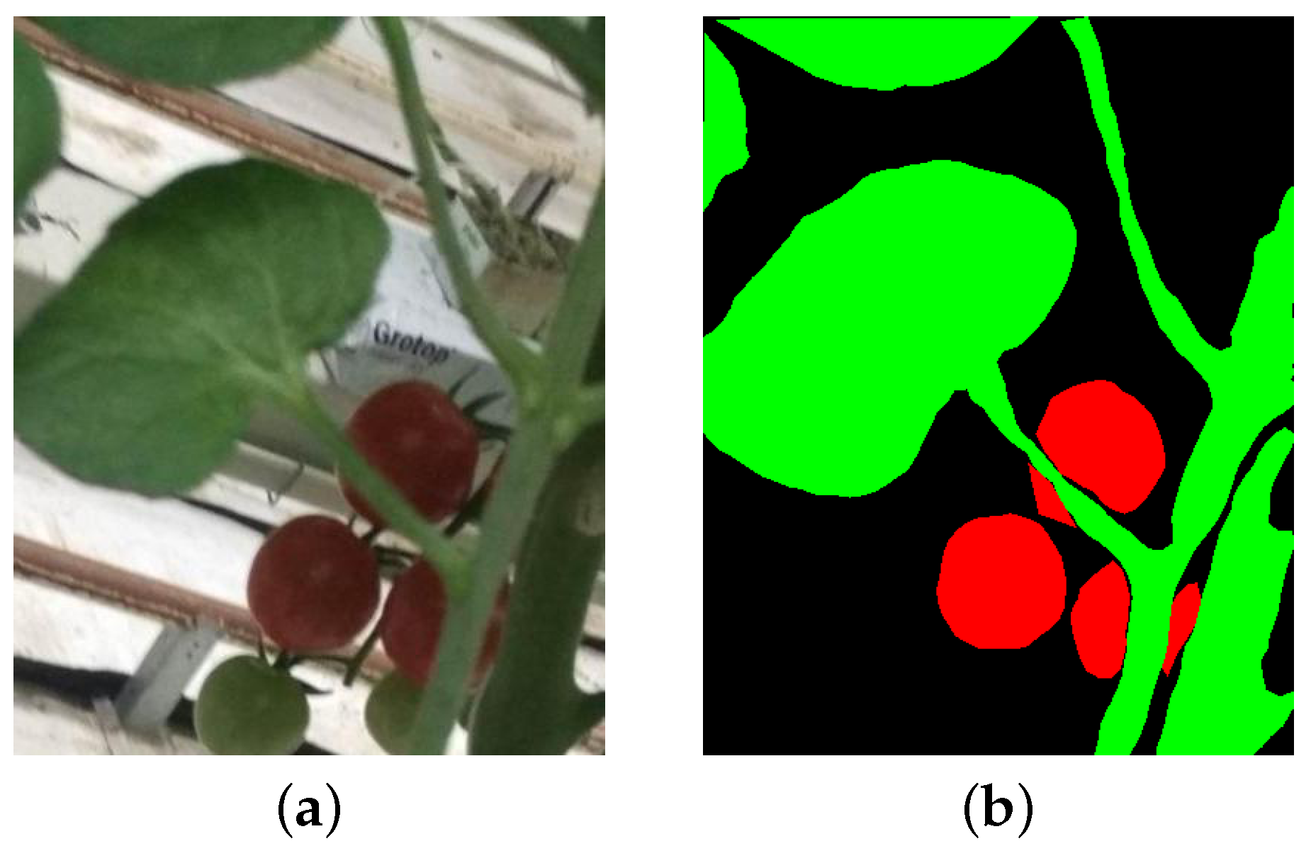
2.1. Segmentation Method by Color Dominance

The process of dividing the elements within images into more easily analyzable sections is known as segmentation [27,28]. The color dominance segmentation method (CDSM),presented in [22], operates in the RGB color space, highlighting the dominance of green in leaves and red in ripe tomato fruits. It is a process to classify pixels into three different classes: the first is the leaves, the second is the fruit, and the last one is the background, which is performed in two stages using threshold-based segmentation.

The CDSM uses the RGB color model; it is important to remember that an image is the representation of a two-dimensional function $f(x,y)$, where x and y represent the spatial coordinates in a Cartesian plane of a pixel. The segmentation method uses the color model RGB, which handles the primary colors red (R), green (G), and blue (B) by the elements: $f_R(x,y)$, $f_G(x,y)$, and $f_B(x,y)$, where the subscript refers to each primary color, respectively. The first stage performs a comparison of the green color channel for the leaves against the other two channels; if the value of the green channel is higher, a pixel belonging to the leaves is determined, and this is stored in the function $h(x,y)$, while for the pixels that make up the fruits, a similar operation is performed, but looking for the pixels whose value of the red channel is higher than the other two, the filtered pixels are stored in the function $j(x,y)$.

The purpose of the second stage is to reduce as much as possible errors in pixel classification generated in the first stage. It begins with the calculation of the differences between the dominant color channel minus non-dominant channels in $h(x,y)$ and $j(x,y)$.

The values of thresholds $U_G^R(x,y)$ and $U_G^B(x,y)$, which determine the final segmentation of pixels corresponding to leaves, while $U_R^G(x,y)$ and $U_R^B(x,y)$ are used in the final segmentation of the pixels that belong to the fruits, observe the following Equations:

$$U_G^R(x,y)={\displaystyle \frac{h_G(x,y)}{M_G}}\ast {\sigma }_G^R\ast {\alpha }_1,$$

(1)

$$U_G^B(x,y)={\displaystyle \frac{h_G(x,y)}{M_G}}\ast {\sigma }_G^B\ast {\alpha }_1,$$

(2)

$$U_R^G(x,y)={\displaystyle \frac{j_R(x,y)}{M_R}}\ast {\sigma }_R^G\ast {\alpha }_2,$$

(3)

$$U_R^B(x,y)={\displaystyle \frac{j_R(x,y)}{M_R}}\ast {\sigma }_R^B\ast {\alpha }_2,$$

(4)

where $M_G$ is the highest value in the green color channel, while $M_R$ is the highest value in the red channel in $h(x,y)$ and $j(x,y)$, respectively. ${\sigma }_G^R$, ${\sigma }_G^B$, ${\sigma }_R^G$, and ${\sigma }_R^B$ correspond to the standard deviations of the ${\Delta }_G^R$, ${\Delta }_G^B$, ${\Delta }_R^G$, and ${\Delta }_R^B$ values, which are the differences of the dominant color channel minus the non-dominate channels, respectively. Finally, values of ${\alpha }_1$ and ${\alpha }_2$ are the factors used to adjust the thresholds in order to improve leaf and fruit segmentation results.

The image $h_F(x,y)$ with the pixels that make up the leaves filtered from $h(x,y)$$\forall x=0,1,2,\dots ,M$ and $\forall y=0,1,2,\dots ,N$ is obtained by

$$h_F(x,y)=\left\{\begin{array}{ccccc}h(x,y)\hfill & if& ({\Delta }_G^R(x,y)>U_G^R(x,y))& and& \left({\Delta }_G^B(x,y)\right)>U_G^B(x,y)\left)\right)\\ \\ 0\hfill & in& another& case\end{array}\right..$$

(5)

The image $j_F(x,y)$ with the pixels that make up the fruits filtered from $j(x,y)$, $\forall x=0,1,2,\dots ,M$ and $\forall y=0,1,2,\dots ,N$ is obtained by:

$$j_F(x,y)=\left\{\begin{array}{ccccc}j(x,y)\hfill & if& (({\Delta }_G^R(x,y)>U_G^R(x,y))& and& ({\Delta }_G^B(x,y)>U_G^B(x,y)))\\ \\ 0\hfill & in& another& case\end{array}\right..$$

(6)

It is important to note that the efficiency of the segmentation performed by the CDSM depends on the values of the color threshold parameters ${\alpha }_1$ and ${\alpha }_2$ used in Equations (1) through (4). A sequential search of these values requires excessive computational power, especially when the size of the image set is large. Therefore, it is necessary to explore alternative methods to determine the values of ${\alpha }_1$ and ${\alpha }_2$, as suggested in the original method [22]. A possible alternative is the use of numerical methods such as polynomial interpolation, which will be described in detail in the following sections, to find an estimate close to the optimal values of the ${\alpha }_1$ and ${\alpha }_2$ parameters with the advantage of saving computational time.

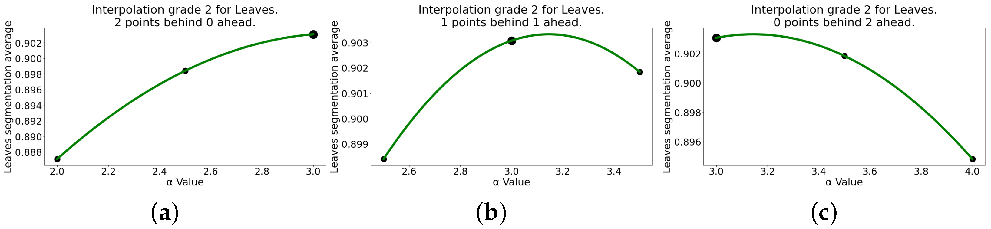
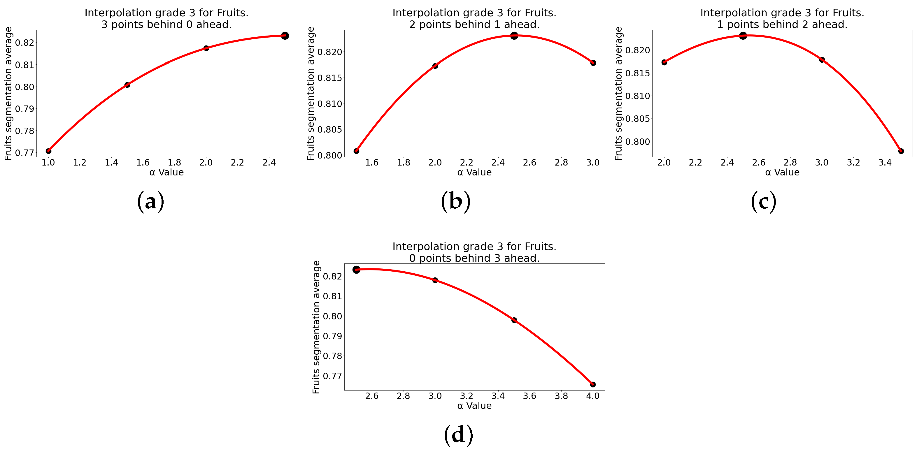
2.2. Unique Interpolation Polynomial (UIP)

A common problem is the estimation of intermediate points between pairs of points in the form $(x,y)$. A polynomial of degree n requires $n+1$ pairs of points to generate a polynomial of the form:

$$P\left(x\right)=a_0+a_{1}x+a_2{x}^2+\cdots +a_n{x}^n.$$

(7)

There are several methods in the literature for generating polynomials, including Newton’s and Lagrange’s methods. While these are effective at estimating intermediate values between points, they have the drawback of not producing a polynomial in the form of Equation (7).

Given a set of $n+1$ points in the form $[(x_0,y_0),(x_1,y_1),\cdots ,(x_{n+1},y_{n+1})]$, it is possible to construct a system of equations similar to

$$\begin{array}{c}\hfill P\left(x_0\right)=a_0+a_1{x}_0+a_2{x}_0^2+\cdots +a_n{x}_0^n\\ \hfill P\left(x_1\right)=a_0+a_1{x}_1+a_2{x}_1^2+\cdots +a_n{x}_1^n\\ \hfill ⋮\\ \hfill P\left(x_n\right)=a_0+a_1{x}_n+a_2{x}_n^2+\cdots +a_n{x}_n^n\end{array}$$

(8)

The x’s represent the known points, and the a’s are the unknowns. Since the number of equations matches the number of unknowns, we can rewrite them as a system of equations in the form:

$$\left[\begin{array}{c}P\left(x_0\right)\\ P\left(x_1\right)\\ ⋮\\ P\left(x_n\right)\end{array}\right]=\left[\begin{array}{ccccc}1& x_0& x_0^2& \cdots & x_0^n\\ 1& x_1& x_1^2& \cdots & x_1^n\\ ⋮& ⋮& ⋮& \cdots & ⋮\\ 1& x_n& x_n^2& \cdots & x_n^n\end{array}\right]\left[\begin{array}{c}{a}_0\\ a_1\\ ⋮\\ a_n\end{array}\right]$$

(9)

Then, the proposed method optimizes the color threshold parameters $\alpha$ for leaf and fruit segmentation using polynomial interpolation. CDSM generates a point set with varying ${\alpha }_1$ and ${\alpha }_2$ values, and UIP is applied to find the optimal values that maximize segmentation results. Solving the system of equations described in Equation (9), where $a_0$ to $a_n$ are the values of the coefficients that generate the curve that describes the behavior of the segmentation with the different values of ${\alpha }_1$ and ${\alpha }_2$.

2.3. Dataset

The dataset used in the experiments of this work, titled “Tomato Detection”, is available at https://www.kaggle.com/datasets/andrewmvd/tomato-detection (accessed on 10 July 2024) and contains nearly 900 images of tomato plants grown in greenhouses Figure 1a shows an example of the images in the dataset. The site hosting the dataset does not provide information on factors such as lighting conditions, capture device, or type of lighting. However, it is evident from the images that they were taken in various environments, at different times of day, and under natural sunlight.

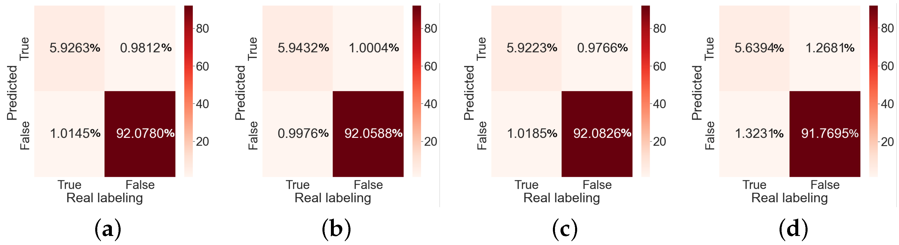
2.3.1. Performance Metrics

Dataset image labeling is crucial for implementing performance metrics, as it provides a basis for quantitatively contrast the results of a segmentation method against images with manual annotations of the elements of interest. This process, known as labeling, can be carried out using various available tools.

In our case, image labeling was performed using the web tool called computer vision annotation tool (CVAT), which is available from the https://www.cvat.ai/ (accessed on 10 July 2024). CVAT is a free tool to perform different labeling functions for applications such as recognition, detection, and segmentation. Figure 1b shows the image masks: the leaves are labeled in green, the fruits in red, and the image background in black.

The term confusion matrix refers to a matrix representation of the prediction results of a binary test. It is used to assess the performance of a classification model on a test dataset where the true outcomes are already known. Each classification result is categorized as either positive (P) or negative (N). The classification within the confusion matrix should be into one of four elements:

• True-Positive $\left(TP\right)$ are pixels that the segmentation algorithm classifies as belonging to a class and in the mask if they belong to this class.
• True-Negative $\left(TN\right)$ are pixels that the segmentation algorithm classifies as not belonging to a class and in the mask do not belong to this class.
• False-Positive $\left(FP\right)$ are pixels that the segmentation algorithm classifies as belonging to a class and in the mask are not.
• False-Negative $\left(FN\right)$ are pixels that the segmentation algorithm classifies as not belonging to a class, and in the mask they are.

Selected metrics are Accuracy, Precision, Recall, and F1-Score [29], and Intersection over Union [30], which are the metrics used to measure the performance of an image segmentation method. During the experimentation stage, the average of the five metrics is used as the target to be optimized.

The Accuracy metric is expressed as:

$$Accuracy={\displaystyle \frac{TP+TN}{TP+TN+FP+FN}}.$$

(10)

The Precision metric defines as:

$$Precision={\displaystyle \frac{TP}{TP+FP}}.$$

(11)

The Recall metric is expressed as:

$$Recall={\displaystyle \frac{TP}{TP+FN}}.$$

(12)

The F1-Score metric is calculated by the expression:

$$F1\text{-}Score=2\ast {\displaystyle \frac{precision\ast recall}{precision+recall}}.$$

(13)

The IoU metric is expressed as:

$$IoU={\displaystyle \frac{TP}{TP+FP+FN}}.$$

(14)

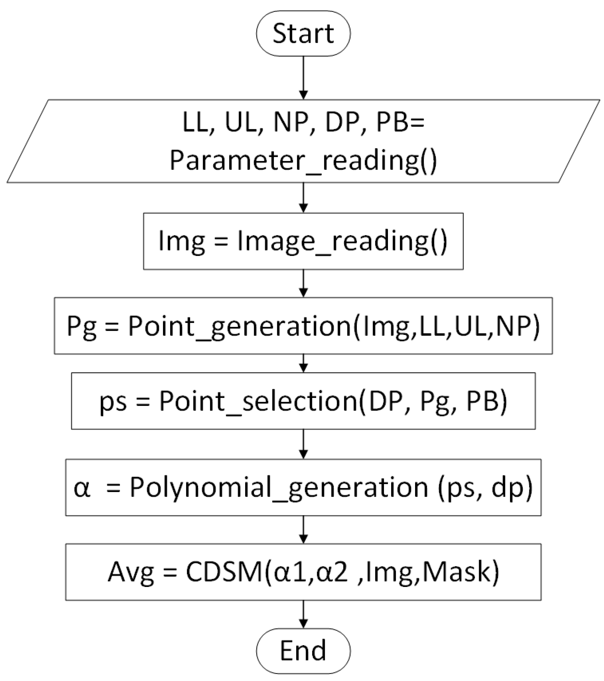
2.4. Polynomial Optimization Method

In reference [22], the color threshold parameter $\alpha$ is employed to optimize the segmentation of tomato plant leaves and fruits. The optimal value of $\alpha$ was determined using a trial-and-error approach until the value that maximized the segmentation results was identified. This approach involved exploring a wide range of values, which required a significant amount of time to test various options.

The polynomial optimization method (POM) proposed in this research is implemented in two stages. In the first one, CDSM is applied with two parameters, ${\alpha }_1$ and ${\alpha }_2$, to maximize the segmentation results. Various values ranging from LL to UL are tested for these parameters, with each value increased by a fixed amount to generate the next test value. For each $\alpha$, the average of the five metrics described in Section 2.3.1 is calculated by segmenting the images, resulting in a set of ordered pairs ($\alpha$, average). This first stage provides the data necessary for performing the polynomial interpolation in the second stage.

The second stage uses a UIP process taking $n+1$ data of the set of ordered pairs generated in the first stage, being n the degree of the desired polynomial. The points to interpolate are selected based on the positions of the ordered pairs with the highest average segmentation, using a specified number of points both before and after these positions until the required number of points for the polynomial degree is reached. The way in which the points to be interpolated are selected is explained in detail in the function Point_selection. Figure 2 illustrates the general procedure of the POM.

Five parameters are necessary to perform the POM to indirectly determine the $\alpha$ values that optimize segmentation results using CDSM. The first two parameters are the Lower Limit (LL) and Upper Limit (UL), which define the range of values used to generate the initial set of points. The third parameter, NP, specifies the number of points to be displayed between the LL and UL values. The fourth parameter, DP, represents the degree of the polynomial to be interpolated. The value of the parameter PB determines the starting position of the points relative to the pivot point. If the number of data points needed $(DP+1)$ is not reached after the pivot point, additional data points are taken from before the pivot point until the required number $(DP+1)$ is obtained, completing the number of points necessary for the polynomial interpolation.

The purpose of the Image_reading function is to read the set of images selected for the first stage of the method, which consists of generating a set of points. In the same way, the data corresponding to the images of the masks with the labeling of the elements of interest are loaded, which are used at the time of calculating the accuracy of the segmentation. For the reading of the images, we use the library functions from the OpenCV.

The Point_generation function receives four parameters: the set of images (Img), the lower (LL) and upper limits (UL), and (NP) are the number of values to be tested with the CDSM between the LL and UL values. The averages of the segmentation of the leaves and fruits of the images with the tomato plants of the dataset are used to generate the set of initial points needed for the POM. This function returns the set of ordered pairs of segmentation averages obtained with the different values taken by the parameters ${\alpha }_1$ and ${\alpha }_2$ in the search range from LL to UL. The Algorithm 1 explains the operation of the function Point_generation.

Algorithm 1 Basic Algorithm for generation of initial points

1: function Point_generation($Img,LL,UL,NP$)   2:     ${\alpha }_1=LL$   3:     ${\alpha }_2=LL$   4:     $Step=(UL-LL)/NP$   5:     $P{g}_{leaves}\left[NP\right]\left[2\right]=0$   6:     $P{g}_{leaves}\left[NP\right]\left[2\right]=0$   7:     $P{g}_{fruits}\left[NP\right]\left[2\right]=0$   8:     $P{g}_{fruits}\left[NP\right]\left[2\right]=0$   9:     $n=0$ 10:     for ($n\le NP$) do 11:         $Av{g}_{leaves},Av{g}_{fruits}=CDSM(Img,{\alpha }_1,{\alpha }_2)$ 12:         $P{g}_{leaves}\left[n\right]\left[0\right]={\alpha }_1$ 13:         $P{g}_{leaves}\left[n\right]\left[1\right]=Av{g}_{leaves}$ 14:         $P{g}_{fruits}\left[n\right]\left[0\right]={\alpha }_2$ 15:         $P{g}_{fruits}\left[n\right]\left[1\right]=Av{g}_{fruits}$ 16:         ${\alpha }_1={\alpha }_1+Step$ 17:         ${\alpha }_2={\alpha }_2+Step$ 18:         $n=n+1$ 19:     end for 20:     return $P{g}_{leaves},P{g}_{fruits}$ 21: end function

$P{g}_{leaves}$ and $P{g}_{fruits}$ are a matrix data structure with dimensions $NP\times 2$ that stores the values of ${\alpha }_1$, ${\alpha }_2$, and the average values generated by segmenting the leaves or fruits of tomato plants.

The function point_selection receives four parameters; DP is the degree of the polynomial to be generated; PB is the number of points behind pivot point; and finally $P{g}_{leaves}$ and $P{g}_{fruits}$ are the dataset of ordered pairs delivered by the Point_generation function, its objective is return the set of ordered pairs selected to generate a UIP; its general structure is shown in the Algorithm 2.

The pivot point is defined as the ordered pair with the highest average segmentation value, either for tomato plant leaves or fruits, as applicable. The algorithm’s operation requires additional functions, such as position_of_max_avg, which identifies the position of the pivot point within the data structures $P{g}_{leaves}$ or $P{g}_{fruits}$.

The UIP process to calculate the values of ${\alpha }_1$ and ${\alpha }_2$ that optimize the averages of segmentation of leaves and fruits of the tomato plant is performed in the Polynomial_generation function shown in Algorithm 3. This requires two parameters: the first is the set of ordered pairs, Ps, used for interpolation, and the second is the degree of the polynomial, DP, to be generated. The result of this function is the root of the generated polynomial, which maximizes the results of segmentation process by CDSM.

Algorithm 2 Selection of points to interpolate from $P{g}_{leaves}$ and $P{g}_{fruits}$

function Point_selection($DP,PB,P{g}_{leaves},P{g}_{fruits}$)     $np=DP+1$     $s\leftarrow size\left(P{g}_{leaves}\right)$     $P{s}_{leaves}\left[np\right]\left[2\right]$=0     $P{s}_{fruits}\left[np\right]\left[2\right]$ =0     $i_1=position\_of\_max\_avg\left(P{g}_{leaves}\right)$     $i_2=position\_of\_max\_avg\left(P{g}_{fruits}\right)$     $p_1=i_1-PB$     $p_2=i_2-PB$     $n=0$     for ($n<np$) do         $P{s}_{leaves}\left[n\right]\left[0\right]=P{g}_{leaves}\left[p_1\right]\left[0\right]$         $P{s}_{leaves}\left[n\right]\left[1\right]=P{g}_{leaves}\left[p_1\right]\left[1\right]$         $P{s}_{fruits}\left[n\right]\left[0\right]=P{g}_{fruits}\left[p_2\right]\left[0\right]$         $P{s}_{fruits}\left[n\right]\left[1\right]=P{g}_{fruits}\left[p_2\right]\left[1\right]$         $p_1=p_1+1$         $p_2=p_2+1$         $n=n+1$     end for     return $P{s}_{leaves},P{s}_{fruits}$ end function

Algorithm 3 Basic Algorithm for function polynomial generation

function Polinomyal_generation($Ps,DP$)     $total=DP+1$     $m=Matrix\_generator(Ps,total)$     $coefficients=Equation\_solution\_method\left(m\right)$     $P=unique\_polynomial\_generator\left(coefficients\right)$     $P^{\prime }=derivate\_polynomial\left(P\right)$     $\alpha =find\_roots\left(P^{\prime }\right)$     return $\alpha$ end function

The Polynomial_generation function shown in Algorithm 3 is composed of several subfunctions. The first of these is Matrix_generator, which takes two parameters: the first is the selected points (Ps) for interpolation, and the second is the degree of the desired polynomial. Its purpose is to generate and return a matrix created from the data of the Ps parameters. The second subroutine, called Equation_solution_method, receives the generated matrix and returns the coefficients of the polynomial. The polynomial_generator function returns the polynomial that is formed with the coefficients that it receives as parameters. The function derivate_polynomial receives as a parameter the polynomial P and returns the first derivative of the polynomial; finally, find_roots delivers the root of the result of equating the derivative to zero and solving the resulting equation. In case there is more than one root, those that are negative are eliminated, and if there are two or more positive roots, they are tested to see which one generates the highest average segmentation.

The color dominance segmentation method is applied in the CDSM function, which requires the parameters ${\alpha }_1$ and ${\alpha }_2$, as well as the sets of images to be segmented and their corresponding masks to be able to carry out the quantitative calculation of the results of the method with the values ${\alpha }_1$ and ${\alpha }_2$. This function is shown in Algorithm 4.

The metric_calculation function receives as a first parameter the result of the segmentation of the leaves or fruits of tomato plants, as well as the data of the mask corresponding to the initial image. As a result, it returns the average of the five metrics described in Section 2.3.1.

Algorithm 4 Color dominance method of segmentation

function CDSM(${\alpha }_1,{\alpha }_2,Img,Mask$)     $s\leftarrow size\left(Img\right)$     $Av{g}_{leaves}=0$     $Av{g}_{fruits}=0$     $i=0$     for ($i<s$) do         $M=Img\left[i\right].number\_of\_rows$         $N=Img\left[i\right].number\_of\_columns$         $h=First\_segmentation\_green\_color\left(Img\right[i\left]\right)$         $j=First\_segmentation\_red\_color\left(Img\right[i\left]\right)$         for ($m<M$) do            for ($n<N$) do                $U_G^R=calculation\_first\_threshold\_green(h(m,n),{\alpha }_1)$                $U_G^B=calculation\_second\_threshold\_green(h(m,n),{\alpha }_1)$                $U_R^G=calculation\_first\_threshold\_red(f(m,n),{\alpha }_2)$                $U_R^B=calculation\_second\_threshold\_red(f(m,n),{\alpha }_2)$                $h_F(m,n)=Final\_green\_color\_segmentation(h,U_G^R,U_G^B)$                $j_F(m,n)=Final\_red\_color\_segmentation(j,U_R^G,U_R^B)$            end for         end for         $Av{g}_{leaves}=Av{g}_{leaves}+metrics\_calculation(h_F,Mask\left[i\right])$         $Av{g}_{fruits}=Av{g}_{fruits}+metrics\_calculation(j_F,Mask\left[i\right])$         $i\leftarrow i+1$     end for     $Av{g}_{leaves}=Av{g}_{leaves}/s$     $Av{g}_{fruits}=Av{g}_{fruits}/s$     return $Av{g}_{leaves},Av{g}_{fruits}$ end function

3. Experimentation and Results

This section outlines the results of the experimentation process, including the number and characteristics of the images used, the computer specifications, the programming language employed, and the key parameters required for implementing the POM.

Experimental Images: For the experimental phase, 300 images and their corresponding masks were used, representing a $33\%$ sample of the dataset. The experimental images used are in portable network graphic (PNG) format and have a resolution of $500\times 400$ pixels. The subset of selected images is not preprocessed before being processed by the proposed method.

Programming language and computer characteristics. Python version $3.9.15$ was selected to implement the proposed algorithm, primarily due to its extensive library support, including OpenCV, which was used for image processing.

The experimentation of the POM method was carried out with a computer with the following specifications:

• Manufacturer: ASUSTeK COMPUTER Inc., Taipei, China
• Modelo: X510UNR
• Processor: Intel^® Core™ i7-8550U CPU @ 1.80GHz × 8.
• RAM: 16 GB.
• Operating system: Ubuntu 22.04.2 LTS 64 bits.

Section 2.4 outlines the method illustrated in Figure 2 for determining the optimal values of ${\alpha }_1$ and ${\alpha }_2$ using the POM. The parameter DP represents the degree of the desired polynomial; in this case, second- and third-degree polynomials were tested. The parameter PB depends on the polynomial degree and ranges from 0 to DP. The initial parameters of the algorithm are listed in

Table 1. Initial general parameter values for interpolation procedure.

General Parameter Initial Values
Parameter	Initial value
Lower limit (LL)	1
Upper limit (UL)	10
NP	18
Second-degree interpolation
DP	2
PB	{2, 1, 0}
Third-degree interpolation
DP	3
PB	{3, 2, 1, 0}

.

Using the parameter values from Table 1, the first stage of the method was conducted, which involves segmenting the leaves and fruits of the tomato plant with different values of ${\alpha }_1$ and ${\alpha }_2$ within the numerical range defined by the LL and UL parameters. The results are presented in

Table 2. Initial values of leaves and fruits segmentation.

Leaves		Fruits
Value ${\mathbf{\alpha }}_{\mathbf{1}}$	Average	Value ${\mathbf{\alpha }}_{\mathbf{2}}$	Average
1	0.82810	1	0.77064
1.5	0.86569	1.5	0.80076
2	0.88711	2	0.81728
2.5	0.89840	2.5	0.82309
3	0.90308	3	0.81783
3.5	0.90184	3.5	0.79786
4	0.89481	4	0.76556
4.5	0.88032	4.5	0.72516
5	0.85739	5	0.67627
5.5	0.82693	5.5	0.63124
6	0.78917	6	0.58066
6.5	0.74334	6.5	0.53069
7	0.69495	7	0.48455
7.5	0.64235	7.5	0.44542
8	0.59173	8	0.40557
8.5	0.53794	8.5	0.37429
9	0.49586	9	0.34096
9.5	0.45202	9.5	0.31707
10	0.41148	10	0.29246

, and their corresponding plots are shown in Figure 3.

For leaves, segmentation with ${\alpha }_1=3.0$ results in an average score of $0.90308$, while for fruits, the best segmentation results are achieved with ${\alpha }_2=2.5$, yielding an average score of $0.82309$. These values represent the optimal segmentation performance across the different ${\alpha }_1$ and ${\alpha }_2$ from LL to UL.

The second stage of the experimentation is tested with polynomials of degree two and three, as well as the selection of different points of the Table 2 taking as axis the values of ${\alpha }_1$ and ${\alpha }_2$ that generate the highest average in the segmentation of leaves and fruits of the tomato plants.

Table 3. Results of different point combinations for second-degree interpolation in leaves segmentation.

Second-Degree Interpolation for Leaves
Points	Points	Polynomial	Derivative	Value α1	Generated Value	Real Segmenting
Behind	Ahead	f(x)	f′(x)	Root	f(α1)	Avg.
2	0	$-0.01324x^2+0.08218x+0.77571$	$-0.02648x+0.08218$	$3.10295$	$0.90321$	$0.90325$
1	1	$-0.01181x^2+0.07431x+0.78643$	$-0.02362x+0.07431$	$3.14566$	$0.90332$	$0.90329$
0	2	$-0.01161x^2+0.07300x+0.78856$	$-0.02322x+0.07300$	$3.14384$	$0.90331$	$0.90329$

,

Table 4. Results different combinations of points for second-degree interpolation for fruits segmentation.

Second-Degree Interpolation for Fruits
Points	Points	Polynomial	Derivative	Value α2	Generated Value	Real Segmenting
Behind	Ahead	f(x)	f′(x)	Root	f(α2)	Avg.
2	0	$-0.02143x^2+0.10805x+0.68690$	$-0.04286x+0.10805$	$2.52085$	$0.82309$	$0.82310$
1	1	$-0.02213x^2+0.11119x+0.68340$	$-0.04426x+0.11119$	$2.51229$	$0.82309$	$0.82309$
0	2	$-0.02943x^2+0.15131x+0.62871$	$-0.05844x+0.15130$	$2.57121$	$0.82323$	$0.82313$

,

Table 5. Results different combinations of points for third-degree interpolation for leaves segmentation.

Third-Degree Interpolation for Leaves
Points	Points	Polynomial	Derivative	Value α1	Generated Value	Real Segmenting
Behind	Ahead	f(x)	f′(x)	Root	f(α1)	Avg.
3	0	$0.00466x^3-0.04825x^2+0.16853x+0.70569$	$0.01400x^2-0.09650x+0.16853$	$3.44561+0.4i$	$0.90450$	$0.90227$
2	1	$0.00095x^3-0.02038x^2+0.09981x+0.76142$	$0.00285x^2-0.04078x+0.09981$	$3.13788$	$0.90329$	$0.90329$
1	2	$0.00013x^3-0.01433x^2+0.02125x+0.75633$	$0.00040x^2-0.02605x+0.07792$	$3.14459$	$0.90332$	$0.90329$
0	3	$-0.00219x^3+0.01142x^2-0.00708x+0.88071$	$-0.00658x^2+0.02285x-0.00708$	$3.12830$	$0.90322$	$0.90327$

and

Table 6. Results different combinations of points for third-degree interpolation for fruits segmentation.

Third-Degree Interpolation for Fruits
Points	Points	Polynomial	Derivative	Value α2	Generated Value	Real Segmenting
Behind	Ahead	f(x)	f′(x)	Root	f(α2)	Avg.
3	0	$0.00385x^3-0.04453x^2+0.15329x+0.65802$	$0.01155x^2-0.08906x+0.15329$	$2.59323$	$0.82321$	$0.82311$
2	1	$-0.00046x^3-0.01863x^2+0.10257x+0.69040$	$-0.00139x^2-0.03726x+0.10257$	$2.51492$	$0.82309$	$0.82308$
1	2	$-0.00486x^3+0.01458x^2+0.02125x+0.75633$	$-0.01458x^2+0.02866x+0.02125$	$2.53925$	$0.82312$	$0.82314$
0	3	$0.00319x^3-0.05813x^2+0.23665x+0.54496$	$0.00957x^2-0.11627x+0.23665$	$2.58559$	$0.82333$	$0.82313$

contain the following information: The first column shows the number of points behind the pivot point, the second column shows the number of points ahead, the third column lists the polynomial created from those selected points, the next column presents the first derivative of the polynomial, the fifth column provides the corresponding root, the sixth column shows the result of evaluating the root in the polynomial, and the final column displays the average segmentation score using the root value.

Table 3 shows the second-degree polynomials generated from the UIP creation process, with the corresponding plots displayed in Figure 4.

The polynomial generated in the experiment using second-degree interpolation for the segmentation of tomato plant fruits is shown in Table 4, with the polynomial plots presented in Figure 5.

Applying the POM with a second-degree polynomial to the case of leaves, the combination that yields the highest average segmentation is 1 point behind and 1 point ahead of the pivot. For fruits, the highest average is achieved by taking 2 points ahead of the pivot point.

For the case of degree three polynomial to estimate the optimal value of ${\alpha }_1$ and ${\alpha }_2$ for the segmentation of leaves and fruits of tomato plants using CDSM. Table 5 contains the results of the polynomial generation using different combinations of points taking as a pivot the value of ${\alpha }_1$, which generates the highest average in the segmentation of tomato leaves. Figure 6 contains the graphs of the polynomials.

Similarly, Table 6 presents the third-degree polynomials generated using the leaf segmentation data. The plots of these polynomials are shown in Figure 7.

When using a third-degree polynomial for leaf segmentation, the combination that yields the best average segmentation is 1 point behind and 2 points ahead of the pivot. For fruits, the highest average segmentation is achieved by taking 2 points behind and 3 points ahead of the pivot point.

The selection of the optimal value for segmenting the leaves and fruits depends directly on the degree of the polynomial. For a second-degree polynomial, the solution has a single root, which is taken as the best value. In contrast, with a third-degree polynomial, the solution provides two roots. If one of these roots has an imaginary component, it is discarded. If both are real, they are tested, and the root that scores highest across the average of five metrics is chosen.

Figure 8 shows the result of the segmentation of leaves and fruits using the values that maximize the average segmentation. Both qualitatively and quantitatively, the clear separation of leaves and fruit pixels from the rest of the image is evident.

It is noteworthy that using the original approach with only one $\alpha$ parameter for optimization yields inferior results compared to using two parameters. Data from Table 2 show that with $\alpha =3.5$, the results are less effective than those obtained by applying the color dominance segmentation method with UIP.

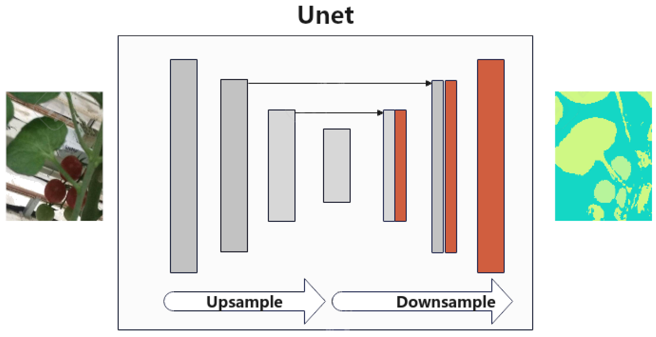
4. Comparison of Results Between Interpolation Procedure vs. Greedy Algorithm vs. UNet CNN

Greedy algorithm is an approach that takes the optimal decision at each stage of the problem with the goal of finding the global optimum at the end of its execution [31]. These are applied in problems where the solution can be constructed sequentially, at each stage choosing values that maximize some objective function. Although the greedy approach does not guarantee the optimal solution, it is a simple and efficient way to solve many problems, with the disadvantage that they are usually slow. Greedy algorithm used to determine the optimal values of ${\alpha }_1$ and ${\alpha }_2$ shown in Algorithm 5, which is an improvement of the gourmand algorithm presented in [32].

Algorithm 5 Greedy algorithm for determining the optimal values of ${\alpha }_1$ and ${\alpha }_2$

1: function Greedy_algorithm($Img,LLl,ULl,LLf,ULf,step,sc$)   2:     while $(step\ge sc)$ do   3:         ${\alpha }_1=LLl$   4:         ${\alpha }_2=LLf$   5:         $NP=(ULl-LLl)/step$   6:         $P{g}_{leaves}\left[NP\right]\left[2\right]=0$   7:         $P{g}_{leaves}\left[NP\right]\left[2\right]=0$   8:         $P{g}_{fruits}\left[NP\right]\left[2\right]=0$   9:         $P{g}_{fruits}\left[NP\right]\left[2\right]=0$ 10:         $n=0$ 11:         while $({\alpha }_1\le LLl)$ do 12:            $Av{g}_{leaves},Av{g}_{fruits}=CDSM(Img,{\alpha }_1,{\alpha }_2)$ 13:            $P{g}_{leaves}\left[n\right]\left[0\right]={\alpha }_1$ 14:            $P{g}_{leaves}\left[n\right]\left[1\right]=Av{g}_{leaves}$ 15:            $P{g}_{fruits}\left[n\right]\left[0\right]={\alpha }_2$ 16:            $P{g}_{fruits}\left[n\right]\left[1\right]=Av{g}_{fruits}$ 17:            ${\alpha }_1={\alpha }_1+step$ 18:            ${\alpha }_2={\alpha }_2+step$ 19:            $n=n+1$ 20:         end while 21:         $step=step/10$ 22:         $LLl,ULl=find\_next\_search\_range\left(P{g}_{leaves}\right)$ 23:         $LLf,ULf=find\_next\_search\_range\left(P{g}_{fruits}\right)$ 24:     end while 25:     return $EntroSliceAtualIP$ 26: end function

Algorithm 5 requires several parameters for execution. The first parameter is the set of images ($Img$) to be segmented along with their masks. $LLl$ and $ULl$ are the minimum and maximum values of the search range for the parameter ${\alpha }_1$, while $LLf$ and $ULf$ are the minimum and maximum values for ${\alpha }_2$. It is important to note that the initial search space for ${\alpha }_1$ and ${\alpha }_2$ in the first iteration of the algorithm must be the same, meaning $LLl=LLf$ and $ULl=ULf$. The step value represents the increment applied to ${\alpha }_1$ and ${\alpha }_2$ within the search space; this value is reduced as different search spaces are explored. The parameter $sc$ denotes the stopping condition, which also serves as the algorithm’s error rate.

Table 7. Initial values for the greedy algorithm.

General Parameter for Greedy Algorithm
Parameter	Initial value
Lower limit for leaves (LLl)	1
Upper limit for leaves (ULl)	10
Lower limit for fruit (LLf)	1
Upper limit for fruit (ULf)	10
step	$0.5$
sc	$0.00005$

shows the values of the execution parameters of the greedy Algorithm 5.

The finds_next_search_range function takes as input the ordered pairs $(\alpha ,AVG)$ for leaves or fruit segmentations within the current search range. It identifies the value of ${\alpha }_1$ or ${\alpha }_2$ that produces the highest average segmentation and then returns the corresponding $\alpha$ value one position back as the new lower bound and the $\alpha$ value one position forward as the new upper bound.

The greedy algorithm required 5 iterations when processing the 300 images selected for the experimental stage; processing each value of ${\alpha }_1$ and ${\alpha }_2$ in a given numerical range takes about 25 min, a total time of 125 min. The greedy algorithm delivers the values of ${\alpha }_1=3.14190$ and ${\alpha }_2=2.57940$ and their respective averages of $0.90329$ and $0.82317$ when segmenting the leaves and fruits at the end of its execution. The described greedy algorithm is currently under review in the “Computación y Sistemas” journal.

Table 8. Comparison of leaf segmentation results of interpolation grade two and three method versus greedy algorithm.

Comparison of Leaves Segmentation Results of Interpolation Method vs. Greedy Algorithm
Greedy algorithm
Optimum value of ${\alpha }_1$ real (AR)		Real avg. (RA)
3.141900		0.903296
Interpolation procedure
Degree polynomial	Calculated ${\alpha }_1$ (CA)	Generated avg. (GA)	Error ${\alpha }_1$ ${(AR-CA)}^2$	Error segmentation $abs(RA-GA)$
2	3.145660	0.903291	$0.000014$	$0.000005$
3	3.137880	0.903292	$0.000016$	$0.000004$

contains the comparison of the greedy algorithm against the proposed interpolation optimization method applying second- and third-degree.

In the case of leaf segmentation, the third-degree polynomial provides better segmentation results than the second-degree polynomial. It is noteworthy that the result obtained using the root of the derivative of both polynomials is nearly identical to the result generated by the greedy algorithm.

For tomato fruit segmentation,

Table 9. Comparison of fruits segmentation results of interpolation grade tow and three method vs. greedy algorithm.

Comparison of Fruits Segmentation Results of Interpolation Method vs. Greedy Algorithm
Greedy algorithm
Optimum value of ${\alpha }_2$ real (AR)		Real avg. (RA)
2.57940		0.823170
Interpolation procedure
Degree polynomial	Calculated ${\alpha }_2$ (CA)	Generated avg. (GA)	Error ${\alpha }_2$ ${(AR-CA)}^2$	Error segmentation $abs(RA-GA)$
2	$2.57121$	$0.823139$	$0.000067$	$0.000031$
3	$2.53925$	$0.823135$	$0.001612$	$0.000035$

presents a comparison between the results of the greedy algorithm and the POM, using both second-degree and third-degree polynomials, similar to the leaf segmentation process.

The second-degree polynomial with 0 points behind and 2 points ahead of the pivot generates better results for segmenting tomato fruits compared to the third-degree polynomial with 2 points behind and 1 point ahead of the pivot. When comparing these results to those of the greedy algorithm, they are virtually identical. Comparing the total time required, the greedy algorithm takes 125 min, whereas generating the initial data requires only 25 min, resulting in an $80\%$ reduction in time when using either the second-degree or third-degree polynomial.

When performing segmentation with the value of $\alpha =3.5$, as reported in [22], on the image set used in this research, better performance was achieved by using two parameters instead of one, resulting in improved average segmentation of the leaves and fruits of tomato plants.

On the other hand, deep learning (DL) is positioned as one of the tools with the greatest potential within artificial intelligence; different models have been developed to meet specific requirements. In 2015, the UNet model was developed to perform segmentation tasks using $100\%$ convolutional layers, primarily for medical images [33]. The UNet comprises two stages: the first one is responsible for encoding the information within the image to comprehend the contextual understanding, achieved through consecutive layers of convolution followed by max-pooling operations. The second stage aims to symmetrically expand the encoded information from the first stage to accurately localize pixels through a series of transposed convolutions. Refer to Figure 9 for the UNet architecture.

During the training process, the weights connecting the layers of the CNN UNet model are adjusted. The models utilize a ResNet50 backbone, a 50-layer recurrent network [34], previously trained with the ImageNet dataset. The account has over 14 million images labeled in over 1000 classes. For the latter, the parameter encoder_freeze is set to True to freeze the weights of the backbone network. The Adam optimizer is utilized, and the models are trained for a total of 50 epochs with a learning rate of $0.01$. The batch size is set to 16, and the training is conducted using the computing equipment specified in the corresponding section. Two groups of images were used for training, the training group with 180 elements and validation with 60, each with their respective images with their corresponding labeling.

When comparing the results of the semantic segmentation done by the UNet model of the leaves and fruits of tomato plants, we found that it has a lower performance compared to the greedy algorithm and the POM; the average of the five metrics for the leaves is $0.880544$, while that of the fruits is $0.819766$.

Table 10. Comparison of the avgs. of the segmentation of the five metrics generated by the compared methods.

Method	Leaves	Fruits
POM Second-degree	0.903291	0.823139
POM Third-degree	0.903292	0.823135
Greedy algorithm	0.903296	0.823170
Unet	0.880544	0.819766

presents the results of the compared methods, while Figure 10 and Figure 11 display their respective confusion matrices represented as heat maps. In these plots, the upper left quadrant indicates the percentage of pixels labeled as true positives (TP), the upper right quadrant shows false positives (FP), the lower left quadrant represents false negatives (FN), and the lower right quadrant illustrates the percentage of true negatives (TN).

5. Practical Applications

The optimized method for segmenting leaves and fruits that we have presented has various applications in the field of precision agriculture. Some of the most relevant include:

• Crop Monitoring: Efficient segmentation of leaves and fruits allows farmers to more accurately track the condition of their crops, facilitating early detection of issues such as diseases or pests.
• Irrigation and Fertilization Optimization: With a more detailed analysis of vegetation, farmers can adjust irrigation and fertilization practices more effectively, optimizing resource use and improving crop yields.
• Precision Harvesting: Accurate segmentation aids in planning harvests, enabling identification of the optimal time for collection and reducing damage to the plants.
• Plant Health Analysis: By differentiating between healthy and unhealthy leaves, the method can be used to assess the overall health of plants and make informed decisions about crop management.

Color-based segmentation algorithms have scientific and practical applications in a wide range of fields, especially in the field of health, by analyzing images from different sources such as magnetic resonance imaging, autonomous vehicle navigation, and factory inspection lines, among others.

6. Conclusions

By using different values for leaves and fruit segmentation in tomato plant images with CDSM, the average of the five performance metrics improves, with a more noticeable increase for fruits when compared to the results of the originally proposed method [22]. The POM proposed in the research is considered successful, highlighting the fact that the images used in the experimentation are acquired in uncontrolled or at least unknown conditions, which implies that by controlling conditions such as lighting, capture device, and angle, among others, better results will be obtained.

By employing second- and third-degree polynomial experiments, we achieve nearly identical performance for segmenting leaves and fruits with selected images. With the processed images, the grade three comparison is better than grade two, and the time required is practically the same. The method for finding the optimal values of ${\alpha }_1$ and ${\alpha }_2$ using interpolation techniques yields results similar to those obtained through iterative optimization by a greedy algorithm and better than the UNet model without the need for specialized hardware for training, as is the case with CNNs.

The main objective of the research was to achieve a time saving in determining the optimal values ${\alpha }_1$ and ${\alpha }_2$ of the alphas, which was achieved by comparing it with the greedy algorithm of about $80\%$ and without the need for a training process as is the case. In the case of the UNet model, it takes about 8 h with a video card; if this is not the case, the time increases considerably.

6.1. Limitations

One factor that directly affects the measurement of leaf and fruit segmentation averages in tomato plants when applying CDSM is the potential for human error during the labeling stage. Such errors impact the results obtained by both the POM and the greedy algorithm. Another limitation of the method is the challenge in identifying weeds, as they share the same green color. However, in the experimental stage presented here, this is not a significant source of error, since the samples come from semi-hydroponic crops where the presence of weeds is minimal. Additionally, unripe fruits, which are also green, can lead to false positives when identifying leaves. These limitations will be addressed in a subsequent stage by incorporating shape and texture recognition algorithms.

6.2. Future Work

Additionally, this method can be extended to other crops that share similar colors, such as strawberries and red bell peppers, where the values of ${\alpha }_1$ and ${\alpha }_2$ could potentially be used without requiring specific adjustments. Likewise, for crops that do not share the colors used in this research, color characterization will be employed, particularly for the fruits. In future work, exploring other numerical methods, such as spline interpolation, could provide a better fit for the iteratively generated optimum. Texture and pattern classification algorithms will also be integrated to help distinguish between elements of the same color, particularly the leaves.

References

1. Gebbers, R.; Adamchuk, V.I. Precision agriculture and food security. Science 2010, 327, 828–831. [Google Scholar] [CrossRef] [PubMed]
2. Rorie, R.L.; Purcell, L.C.; Karcher, D.E.; King, C.A. The assessment of leaf nitrogen in corn from digital images. Crop Sci. 2011, 51, 2174–2180. [Google Scholar] [CrossRef]
3. Sun, Y.; Gao, J.; Wang, K.; Shen, Z.; Chen, L. Utilization of Machine Vision to Monitor the Dynamic Responses of Rice Leaf Morphology and Colour to Nitrogen, Phosphorus, and Potassium Deficiencies. J. Spectrosc. 2018, 2018, 1469314. [Google Scholar] [CrossRef]
4. Dhingra, G.; Kumar, V.; Joshi, H.D. A novel computer vision based neutrosophic approach for leaf disease identification and classification. Meas. J. Int. Meas. Confed. 2019, 135, 782–794. [Google Scholar] [CrossRef]
5. Ireri, D.; Belal, E.; Okinda, C.; Makange, N.; Ji, C. A computer vision system for defect discrimination and grading in tomatoes using machine learning and image processing. Artif. Intell. Agric. 2019, 2, 28–37. [Google Scholar] [CrossRef]
6. Wang, Y.; Wang, D.; Zhang, G.; Wang, J. Estimating nitrogen status of rice using the image segmentation of G-R thresholding method. Field Crop. Res. 2013, 149, 33–39. [Google Scholar] [CrossRef]
7. Kirk, K.; Andersen, H.J.; Thomsen, A.G.; Jørgensen, J.R.; Jørgensen, R.N. Estimation of leaf area index in cereal crops using red-green images. Biosyst. Eng. 2009, 104, 308–317. [Google Scholar] [CrossRef]
8. Sun, Y.; Tong, C.; He, S.; Wang, K.; Chen, L. Identification of Nitrogen, Phosphorus, and Potassium Deficiencies Based on Temporal Dynamics of Leaf Morphology and Color. Sustainability 2018, 10, 762. [Google Scholar] [CrossRef]
9. Castillo-Martínez, M.; Gallegos-Funes, F.J.; Carvajal-Gámez, B.E.; Urriolagoitia-Sosa, G.; Rosales-Silva, A.J. Color index based thresholding method for background and foreground segmentation of plant images. Comput. Electron. Agric. 2020, 178, 105783. [Google Scholar] [CrossRef]
10. Nakane, T.; Bold, N.; Sun, H.; Lu, X.; Akashi, T.; Zhang, C. Application of evolutionary and swarm optimization in computer vision: A literature survey. IPSJ Trans. Comput. Vis. Appl. 2020, 12, 3. [Google Scholar] [CrossRef]
11. Puranik, P.; Bajaj, P.; Abraham, A.; Palsodkar, P.; Deshmukh, A. Human perception-based color image segmentation using comprehensive learning particle swarm optimization. In Proceedings of the 2009 2nd International Conference on Emerging Trends in Engineering and Technology, ICETET, Nagpur, India, 16–18 December 2009; pp. 630–635. [Google Scholar] [CrossRef]
12. Ghamisi, P.; Couceiro, M.S.; Martins, F.M.; Benediktsson, J.A. Multilevel image segmentation based on fractional-order darwinian particle swarm optimization. IEEE Trans. Geosci. Remote Sens. 2014, 52, 2382–2394. [Google Scholar] [CrossRef]
13. Tao, W.B.; Tian, J.W.; Liu, J. Image segmentation by three-level thresholding based on maximum fuzzy entropy and genetic algorithm. Pattern Recognit. Lett. 2003, 24, 3069–3078. [Google Scholar] [CrossRef]
14. Liang, Y.C.; Chen, A.H.L.; Chyu, C.C. Application of a hybrid ant colony optimization for the multilevel thresholding in image processing. In Neural Information Processing, Proceedings of the 13th International Conference, ICONIP 2006, Hong Kong, China, 3–6 October 2006, Proceedings, Part II; Lecture Notes in Computer Science (Including Subseries Lecture Notes in Artificial Intelligence and Lecture Notes in Bioinformatics); Springer: Berlin/Heidelberg, Germany, 2006; Volume 4233, pp. 1183–1192. [Google Scholar] [CrossRef]
15. Vergés-Llahí, J.; Climent, J.; Sanfeliu, A. Colour image segmentation solving hard-constraints on graph partitioning greedy algorithms. Proc.-Int. Conf. Pattern Recognit. 2000, 15, 625–628. [Google Scholar] [CrossRef]
16. Subr, K.; Majumder, A.; Irani, S. Greedy algorithm for local contrast enhancement of images. In Image Analysis and Processing—ICIAP 2005, Proceedings of the 13th International Conference, Cagliari, Italy, 6–8 September 2005. Proceedings 13; Lecture Notes in Computer Science (Including Subseries Lecture Notes in Artificial Intelligence and Lecture Notes in Bioinformatics); Springer: Berlin/Heidelberg, Germany, 2005; Volume 3617, pp. 171–179. [Google Scholar] [CrossRef]
17. Patil, B.M.; Amarapur, B. Segmentation of leaf images using greedy algorithm. In Proceedings of the 2017 International Conference on Energy, Communication, Data Analytics and Soft Computing, ICECDS 2017, Chennai, India, 1–2 August 2018; pp. 2137–2141. [Google Scholar] [CrossRef]
18. Le Guyader, C.; Apprato, D.; Gout, C. Using a level set approach for image segmentation under interpolation conditions. Numer. Algorithms 2005, 39, 221–235. [Google Scholar] [CrossRef]
19. Paiement, A.; Mirmehdi, M.; Xie, X.; Hamilton, M.C. Integrated segmentation and interpolation of sparse data. IEEE Trans. Image Process. 2014, 23, 110–125. [Google Scholar] [CrossRef]
20. Ge, M.S.; Wu, P.T.; Zhu, D.L.; Zhang, L. Application of different curve interpolation and fitting methods in water distribution calculation of mobile sprinkler machine. Biosyst. Eng. 2018, 174, 316–328. [Google Scholar] [CrossRef]
21. Moon, T.; Hong, S.; Choi, H.Y.; Jung, D.H.; Chang, S.H.; Son, J.E. Interpolation of greenhouse environment data using multilayer perceptron. Comput. Electron. Agric. 2019, 166, 105023. [Google Scholar] [CrossRef]
22. Guerra Ibarra, J.P.; Cuevas, F.J. Segmentation of Leaves and Fruits of Tomato Plants by Color Dominance. AgriEngineering 2023, 5, 1846–1864. [Google Scholar] [CrossRef]
23. Li, J.; Zhang, F.; Qian, X.; Zhu, Y.; Shen, G. Quantification of rice canopy nitrogen balance index with digital imagery from unmanned aerial vehicle. Remote Sens. Lett. 2015, 6, 183–189. [Google Scholar] [CrossRef]
24. Nagar, H.; Sharma, R. Pest Detection on Leaf using Image Processing. In Proceedings of the 2021 International Conference on Computer Communication and Informatics (ICCCI), Coimbatore, India, 27–29 January 2021; IEEE: Piscataway, NJ, USA, 2021; pp. 1–5. [Google Scholar] [CrossRef]
25. Liu, X.; Zhao, D.; Jia, W.; Ji, W.; Ruan, C.; Sun, Y. Cucumber fruits detection in greenhouses based on instance segmentation. IEEE Access 2019, 7, 139635–139642. [Google Scholar] [CrossRef]
26. Kang, H.; Chen, C. Fruit detection and segmentation for apple harvesting using visual sensor in orchards. Sensors 2019, 19, 4599. [Google Scholar] [CrossRef] [PubMed]
27. González Perea, R.; Daccache, A.; Rodríguez Díaz, J.A.; Camacho Poyato, E.; Knox, J.W. Modelling impacts of precision irrigation on crop yield and in-field water management. Precis. Agric. 2018, 19, 497–512. [Google Scholar] [CrossRef]
28. Jaiswal, S.; Pandey, M.K. A Review on Image Segmentation. Adv. Intell. Syst. Comput. 2021, 1187, 233–240. [Google Scholar] [CrossRef]
29. Taheri, M.; Lim, N.; Lederer, J. Balancing Statistical and Computational Precision and Applications to Penalized Linear Regression with Group Sparsity; Department of Computer Sciences and Department of Biostatistics and Medical Informatics: Madison, WI, USA, 2016; pp. 233–240. [Google Scholar]
30. Rezatofighi, H.; Tsoi, N.; Gwak, J.; Sadeghian, A.; Reid, I.; Savarese, S. Generalized intersection over union: A metric and a loss for bounding box regression. In Proceedings of the IEEE Computer Society Conference on Computer Vision and Pattern Recognition, Long Beach, CA, USA, 16–20 June 2019; pp. 658–666. [Google Scholar] [CrossRef]
31. Feo, T.A.; Resende, M.G.C. Greedy Randomized Adaptive Search Procedures. J. Glob. Optim. 1995, 6, 109–133. [Google Scholar] [CrossRef]
32. Guerra Ibarra, J.P.; Cuevas de la Rosa, F. Optimization of Color Dominance Factor by Greedy Algorithm for Leaves and Fruit Segmentation of Tomato Plants. In Pattern Recognition; Mezura-Montes, E., Acosta-Mesa, H.G., Carrasco-Ochoa, J.A., Martínez-Trinidad, J.F., Olvera-López, J.A., Eds.; Springer Nature: Cham, Switzerland, 2024; pp. 200–209. [Google Scholar]
33. Ronneberger, O.; Fischer, P.; Brox, T. UNet: Convolutional Networks for Biomedical Image Segmentation; Springer: Cham, Switzerland, 2015; Volume 9351, pp. 234–241. [Google Scholar] [CrossRef]
34. McNeely-White, D.; Beveridge, J.R.; Draper, B.A. Inception and ResNet features are (almost) equivalent. Cogn. Syst. Res. 2020, 59, 312–318. [Google Scholar] [CrossRef]
Figure 1. (a) Example image of the tomato plantations dataset. (b) Example of mask of (a).
Agriculture 14 01911 g001
Figure 2. Polynomial optimization method.
Agriculture 14 01911 g002
Figure 3. Leaf and fruit segmentation averages with different α 1 and α 2 values from L L = 1 to U L = 10 . (a) Leaf segmentation avg. from L I = 1 to U L = 10 , max avg. with α 1 = 3.0 , (b) Fruits segmentation avg. from L I = 1 to U L = 10 , max avg. with α 2 = 2.5 .
Agriculture 14 01911 g003
Figure 4. Polynomial plots for second-degree interpolation of leaves segmentation. (a) 2 points behind 0 ahead, (b) 1 point behind 1 ahead, (c) 0 point behind 2 ahead.
Agriculture 14 01911 g004
Figure 5. Polynomial plots for second-degree interpolation of fruits segmentation. (a) 2 points behind 0 ahead, (b) 1 point behind 1 ahead, (c) 0 point behind 2 ahead.
Agriculture 14 01911 g005
Figure 6. Polynomial plots for third-degree interpolation of leaves segmentation. (a) 3 point behind 0 ahead, (b) 2 point behind 1 ahead, (c) 1 point behind 2 ahead, (d) 0 point behind 3 ahead.
Agriculture 14 01911 g006
Figure 7. Polynomial plots degree 3 of fruit segmentation. (a) 3 points behind 0 ahead, (b) 2 points behind 1 ahead, (c) 1 point behind 2 ahead, and (d) 0 point behind 3 ahead.
Agriculture 14 01911 g007
Figure 8. Example of segmentation of leaves and fruits of tomato plants. (a) Initial image. (b) Image with leaf segmentation. (c) Image with fruit segmentation.
Agriculture 14 01911 g008
Figure 9. CNN UNet Architecture.
Agriculture 14 01911 g009
Figure 10. Confutation Matrix graphs represented with heat maps of the compared experiments for leaves. (a) Second-degree POMs. (b) Third-degree POMs. (c) Greedy algorithm. (d) UNet model.
Agriculture 14 01911 g010
Figure 11. Confutation Matrix graphs represented with heat maps of the compared experiments for fruits. (a) Second-degree POMs. (b) Third-degree POMs. (c) Greedy algorithm. (d) UNet model.
Agriculture 14 01911 g011