Improved YOLOv5 Network for Detection of Peach Blossom Quantity

Abstract

In agricultural production, rapid and accurate detection of peach blossom bloom plays a crucial role in yield prediction, and is the foundation for automatic thinning. The currently available manual operation-based detection and counting methods are extremely time-consuming and labor-intensive, and are prone to human error. In response to the above issues, this paper proposes a natural environment peach blossom detection model based on the YOLOv5 model. First, a cascaded network is used to add an output layer specifically for small target detection on the basis of the original three output layers. Second, a combined context extraction module (CAM) and feature refinement module (FSM) are added. Finally, the network clusters and statistically analyzes the range of multi-scale channel elements using the K-means++ algorithm, obtaining candidate box sizes that are suitable for the dataset. A novel bounding box regression loss function (SIoU) is used to fuse the directional information between the real box and the predicted box to improve detection accuracy. The experimental results show that, compared with the original YOLOv5s model, our model has correspondingly improved AP values for identifying three different peach blossom shapes, namely, bud, flower, and falling flower, by 7.8%, 10.1%, and 3.4%, respectively, while the final mAP value for peach blossom recognition increases by 7.1%. Good results are achieved in the detection of peach blossom flowering volume. The proposed model provides an effective method for obtaining more intuitive and accurate data sources during the process of peach yield prediction, and lays a theoretical foundation for the development of thinning robots.

1. Introduction

In recent years, with the rapid economic development of the forest and fruit industries, peach trees have been growing in scale and yield as one of the most popular. However, there is room for improvement in the cultivation quality and technical level of peach trees. In the growth cycle of peach trees, in order to improve the yield and quality of peach fruits, in addition to doing well in soil management, fertilization, irrigation, and pest and disease prevention and control, flower management is a crucial link. Studies have shown that under good pollination conditions, the final yield of peach fruits is positively correlated with the flowering quantity [1]. Therefore, the flowering quantity of peach trees can be used as an important indicator for yield prediction, which can help to simplify the arrangement of harvesting labor, other resources (such as orchard platforms), and post-harvest processing strategies while providing a quantitative basis for rational planning of harvesting [2]. Meanwhile, the yield measurement of peach trees can help fruit farmers to grasp the growth status of fruit trees and estimate the economic benefits of orchards. In addition, the yield measurement of peach trees can be used to conduct quantitative analysis of possible losses and provide evidence support for loss assessment in agricultural insurance [3]. Due to the annual changes in flowering quantity and climatic conditions (temperature, precipitation, etc.) during the flowering period, the harvest period yield of the same orchard varies in different years. Therefore, it is necessary to establish a relationship model between flowering quantity, climatic factors, and yield in order to predict the yield from the flowering quantity.

The thinning of peach trees has a significant impact on the yield, quality, and health of peach fruits; thus, choosing a suitable thinning method is an important part of peach flower management. Existing studies have shown that proper thinning can improve the yield and quality of fruits [4,5,6,7], directly affecting their market value. The traditional thinning method relies on manual operation, which is time-consuming and labor-intensive. There are two kinds of thinning methods with higher efficiency: chemical thinning and physical thinning [8,9]. Chemical thinning is restricted by factors such as weather, spraying time, tree age, tree vigor, etc. [10]. With the improvement of people’s living standards and the attention to fruit safety, the demand for reducing or avoiding the use of pesticides and other inorganic substances in fruit production is greatly increasing. Therefore, physical thinning is expected to become the mainstream trend in the future [11]. However, using ropes or other striking devices for mechanical thinning can easily cause damage to the tree or poor thinning effect. Therefore, automatic and precise thinning is expected to be the future development trend, and it is urgent to develop a fast and accurate method for detecting the flowering quantity.

Early studies used traditional image processing algorithms to detect and identify fruit tree flowers; [12] was the first to use computer vision technology to detect flowers, which was based on color thresholding but was only applicable to controlled situations. Krikeb et al. [13] used thresholding and morphological methods to identify flowers and predict the timing and intensity of full bloom. Hočevar et al. [14] used thresholding in the HSL color space to identify apple flowers. Wang [15] used fixed color thresholds to separate flowers, then refined the segmentation results via SVM classification. Wang [16] used pixel color thresholding, then used accelerated robust features for SVM classification to segment mango flowers; however, the applicability of this approach is limited by the changes in illumination conditions and the occlusion of stems, leaves, or other flowers. Most of these methods rely on manually designed features, meaning that their overall performance can only achieve good results in relatively controlled environments, such as artificial lighting on a night curtain-covered background. Flower detection based on traditional image processing algorithms is easily affected by environmental factors such as lighting, shadows, etc., and has poor applicability [17].

Other studies have attempted flower detection based on deep learning; [18] was the first to use CNN for apple flower detection, which was superior to the color-based method, although limited by the inherent inaccuracy of its superpixel segmentation and network architecture. Dias et al. [19] used the DeepLab+RGR model to identify peach and pear flowers. Sun et al. [20] proposed a method using the DeepLab-ResNet network to detect apple, peach, and pear flowers; however, the recognition effect of peach flowers in this method was poor. Wang et al. [21,22] proposed a fully convolutional network-based apple flower segmentation method. Tian et al. [23] successfully applied the single-stage SSD algorithm to detect apple flowers, achieving an average detection accuracy of 87.40%. Farjon et al. [24] used the deep learning-based Faster R-CNN algorithm for object detection, and employed image processing techniques to cluster and count the detected flowers, effectively realizing the automatic estimation of the number of apple flowers. However, these deep learning-based methods are mostly used for detecting flowers in single images. Wu et al. [25] and Tian et al. [26] proposed apple flower detection methods based on the YOLOv4 and MASU R-CNN models, respectively, both of which achieved high detection accuracy. Ye et al. [27] improved the YOLOv5 model by adding a CA attention mechanism and the feature fusion structure to detect pear flowers. Shang et al. [28] used the lightweight YOLO v5s model and added a context extraction module (CAM) to detect apple flowers of various colors under different weather and lighting conditions. Tao et al. [29] proposed a method based on an RGBD camera and convolutional neural network that integrated the attention mechanism and multi-scale feature fusion to detect peach flower density.

As can be seen from the above literature review, deep learning has shown great potential in fruit tree flower recognition and detection and has effectively improved detection performance compared with traditional methods. However, compared with other fruit tree flowers, there are few related recognition studies on peach flowers. Although deep learning-based models have relevant research in the field of peach flower detection, the current research on high-precision classification and detection of peach flowers with different morphologies has not achieved effective results. Taking Figure 1 as an example, the reasons that hinder the development of this process are as follows: (1) peach flower recognition belongs to complex background small object recognition, which is easily affected by the background of branches, leaves, ground, and other fruit trees; (2) peach flowers are divided into three morphologies, namely, buds, flowers, and fallen flowers, meaning that there can be three morphologies of flowers in a stage at the same time, requiring all three morphologies to be classified and recognized; and (3) there are many peach flowers on a peach tree, and there are serious occlusion problems between flowers, meaning that the original flower segmentation method cannot accurately segment all complete flower morphologies.

To address the above problems, this paper proposes a method based on improved YOLOv5s for segmentation of peach flowers with different morphologies and detection of peach blossom quantity. The main contributions of this paper are as follows:

(1)

A peach flower image dataset is constructed (a total of 5000 images) to provide data support for the training and validation of the peach flower detection model.

(2)

An additional layer dedicated to small object detection is added. Because it is fused with shallower feature maps, the new feature map has strong semantic information and precise location information, which can be used to improve the detection rate of buds.

(3)

The combination of a context extraction module (CAM) and a feature refinement module (FSM) is adopted. The CAM module is used to extract context information, while feature refinement through the FSM module can further suppress conflicting information and improve the accuracy of flower detection.

(4)

To improve model performance, the K-means++ algorithm is used to help the initial clustering center escape the local optimum and reach the global optimum, while the SIoU loss function replaces the original CIoU function in order to more fully consider the influence of the vector direction between the ground truth box and the predicted box while providing faster model convergence.

2. Materials and Methods

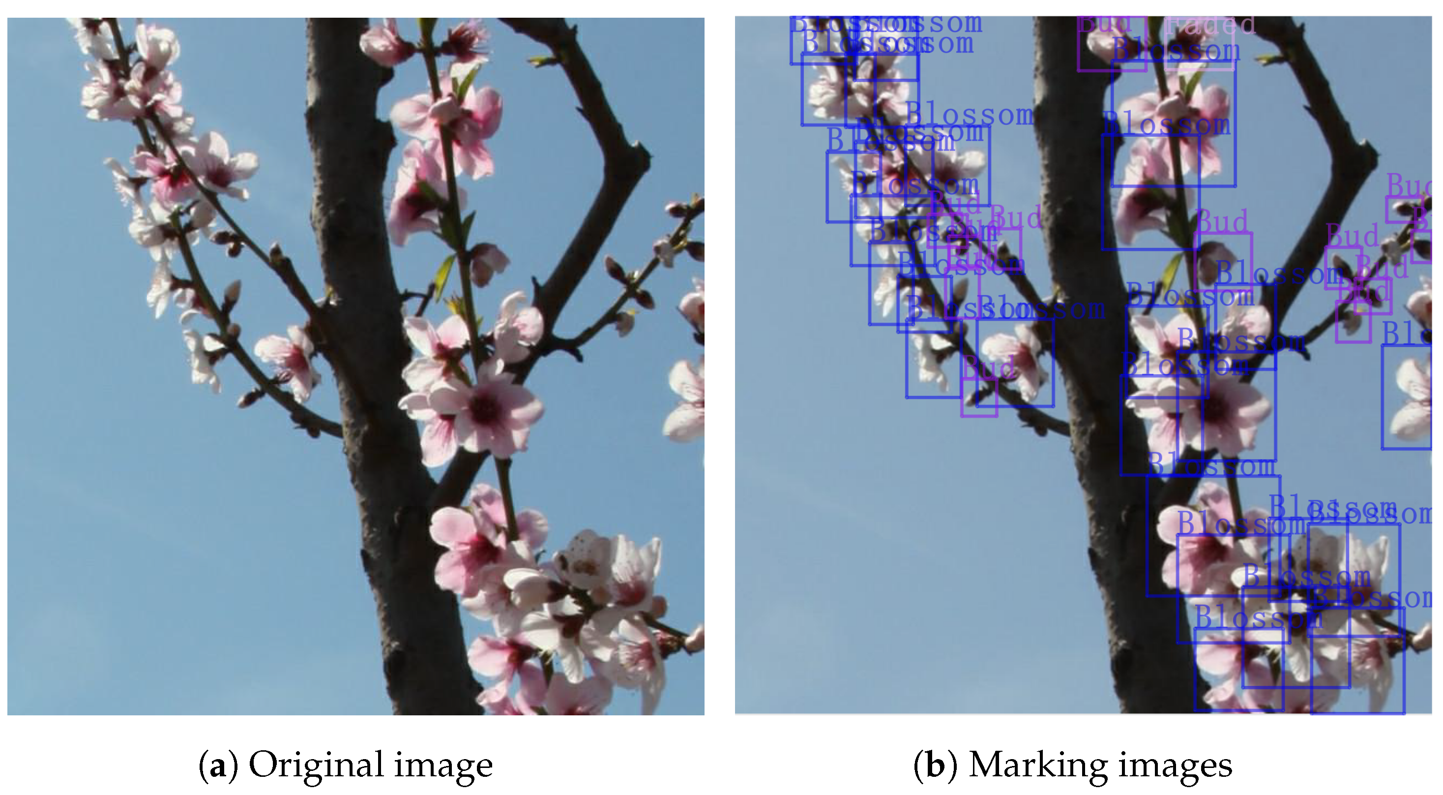
2.1. Image Dataset

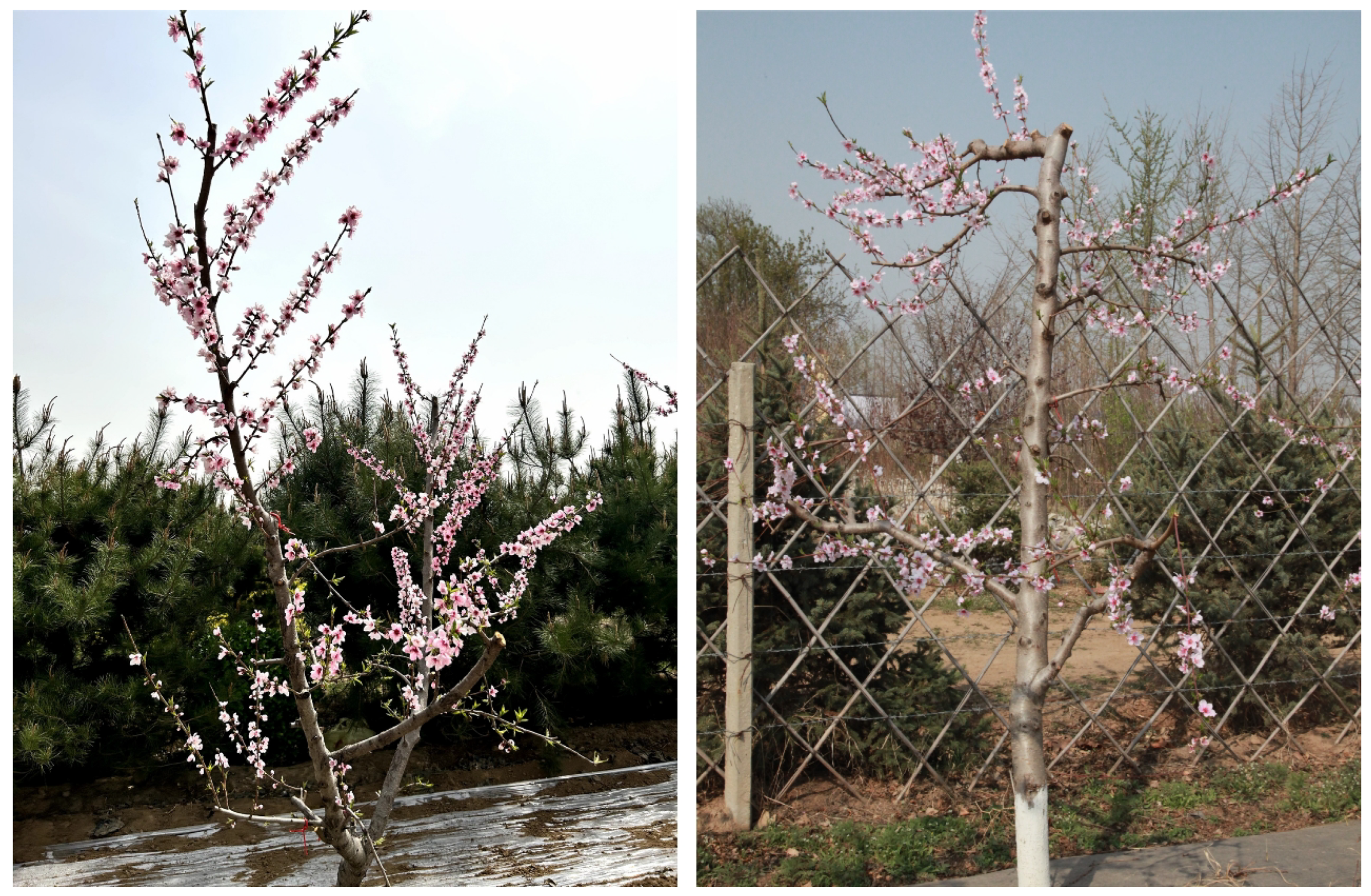
2.1.1. Image Acquisition

The peach blossom image samples used in the experiment were collected from the peach tree breeding base of the Mancheng District Branch of the Natural Resources and Planning Bureau of Baoding. The varieties were 3-year-old “Jiuli”, “Chunxue”, and “Baojiajun”. The cultivation mode of the orchard was arranged in rows from north to south, with a row spacing of 5 m × 3 m. The image acquisition plan was as follows. (1) Shooting period: balloon period, blooming period, and falling period (to ensure that the three forms of flowers have sufficient data volume). (2) Shooting time: from 8:30 to 9:30, 11:00 to 12:00, and 15:00 to 16:00 every day, continuously randomly shot peach blossoms in the experimental area (reducing the impact of different light intensities on recognition performance and increasing generalization ability under different environmental conditions). (3) Shooting subjects: 60 trees were randomly selected in the orchard, and a total of 300 peach blossom images were taken in each period. The experimental data were taken on the front, side, and occlusion images of the peach blossoms (different fruit trees contain different image information in different directions, increasing the richness of the dataset). (4) Shooting distance: in an upward position 2 m away from the peach tree and 1-m-high (to minimize the influence of complex backgrounds). (5) Shooting equipment: the camera used in this study was a Canon 5D paired with a Canon 24–105 mm lens, with an image resolution of 2720 × 4080.

2.1.2. Image Processing

After filtering the original images, a total of 608 images containing the target were obtained, including 198 images during the balloon period, 232 images during the blooming period, and 178 images during the falling period. To adapt to the best recognition performance of the YOLOv5 network model, the collected image size was randomly cropped to 640 × 640 pixels and, if insufficient was filled with RGB (128,128,128). After cropping, we removed sub-images such as sky and land that did not contain peach blossom targets and organized a total of 5000 peach blossom images. The ratio of the training set:testing set:validation set was 7:2:1, respectively. The labeling tool was used to label peach blossoms with three types of labels: Bud, Blossom, and Faded. The areas with flowers in each image were labeled according to their respective flower morphology. The process example is shown in Figure 2b; the purple box represents the position of the flower bud label, the blue box represents the position of the flower label, and the pink box represents the falling flower label. Then, we generated corresponding XML format files containing location information, including the image category name information, and target rectangular box location information. Experts familiar with peach tree cultivation management were responsible for image labeling in order to ensure the accuracy of identification of different flower areas. Finally, the dataset was converted to a VOC2007 format to meet the experimental requirements of Yolov5.

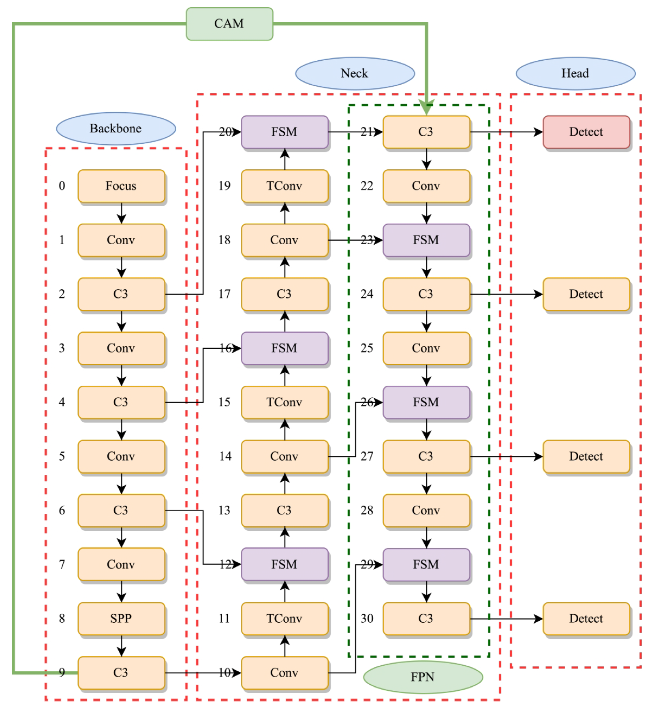
2.2. Research Methods

The YOLO series detection network is an important branch of object detection models, and its application in agricultural object detection is becoming increasingly widespread [30,31,32]. YOLOv5s helps mobile devices to achieve real-time object detection while ensuring the accuracy of object detection [33,34]. Therefore, we used the YOLOv5s network as the basic network for transformation in this experiment.

2.2.1. Small Object Detection Layer

The shape of the flower bud is small and belongs to the category of small object detection. The original multi-scale detection structure is prone to missed detection of such targets. In order to better extract the position information of small targets, the detection layer in YOLOv5 was increased from the original three layers to the current four layers. The specific operation involves continued upsampling and other processing on the feature map after the 16th layer, meaning that the feature map continues to expand. At the same time, at the 20th layer, the obtained feature map with a size of 160 × 160 undergoes tensor splicing and fusion with the feature map of the second layer in the backbone network to obtain a larger feature map for the detection of small target objects. In the 21st layer, which is the detection layer, a small object detection layer (marked in pink in Figure 3) is added. After improvement, the entire model uses a total of four detection layers for detection. The four detection scales utilize both the high-resolution low-level features and the high semantic information of the deep features without significantly increasing network complexity.

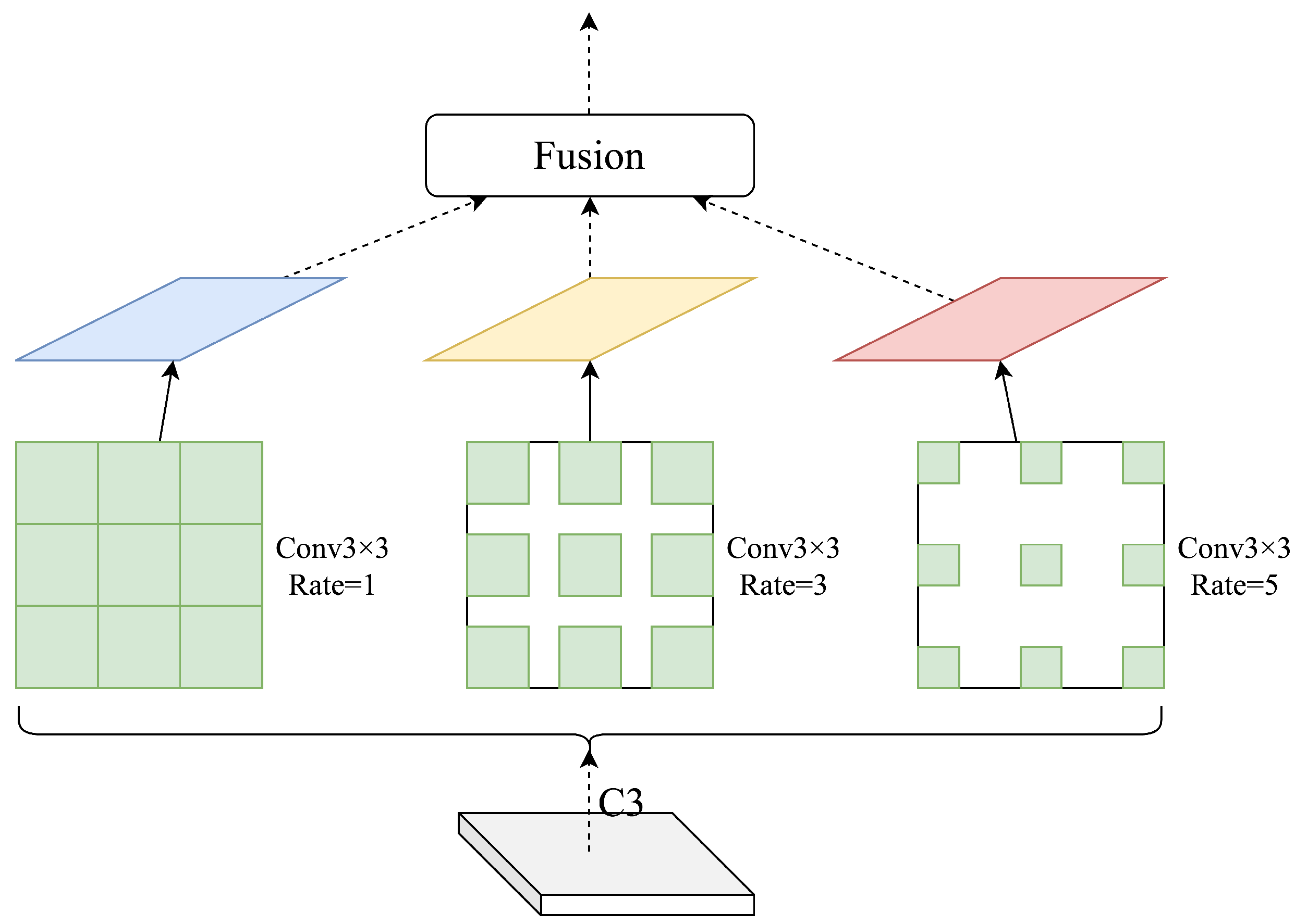
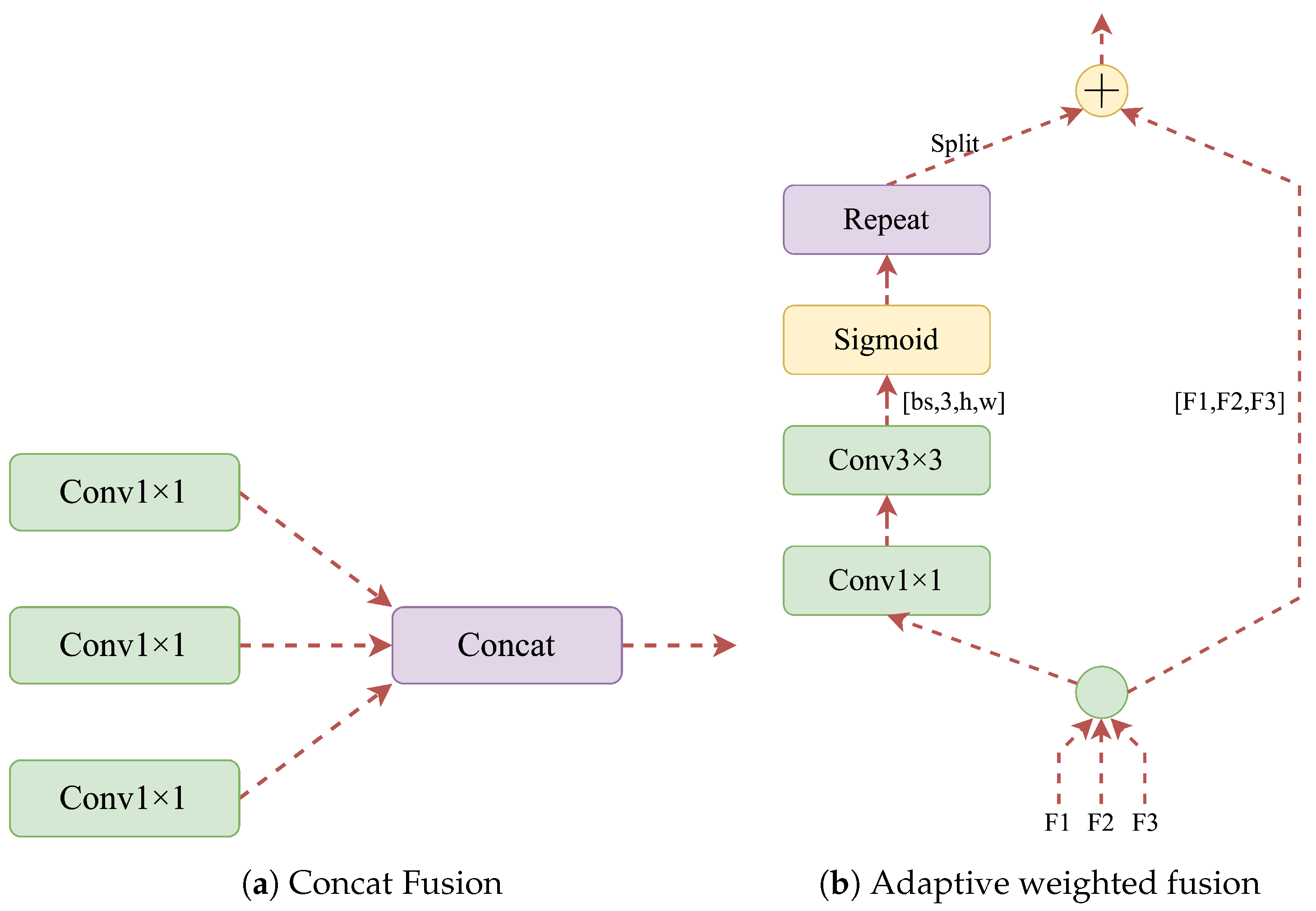
2.2.2. Context Enhancement Module

Small bud detection requires context information. We propose using dilated convolutions with different dilation rates to obtain context information with different receptive fields and enrich the context information of FPN. On the basis of the original neck layer, we added the CAM module [35] (marked in green in Figure 3). The structure of the module is shown in Figure 4).

We obtained context information with different receptive fields by performing dilated convolutions with different dilation rates on the ninth C3 layer. The kernel size was 3 × 3, the dilation rates were 1, 3, and 5, and there were two possible fusion methods, as shown in Figure 5a,b.

Figure 5a shows 1 × 1 convolution on the feature maps after dilated convolution, which enhances learning ability while maintaining the features’ smoothness. Finally, the Concat operation is performed on the three feature maps obtained by convolution. Figure 5b shows the adaptive weighted fusion method, which uses residual branches to inject different spatial context information into the original branches to improve the feature representation. The three inputs are the three outputs of Figure 5a, and the context information is concentrated on the output by calculating the weighted sum. The effectiveness of the two fusion methods is compared by the experiments shown in

Table 1. Ablation experiments on the two fusion methods.

Algorithm	mAP/%	FPS
YOLOv5s	83.1	45.61
YOLOv5s + CAM + concat	86.2	44.89
YOLOv5s + CAM + weight	85.1	44.86

.

As can be seen from Table 1, the addition of the CAM module improves accuracy by at least 2% compared to the original YOLOv5, which proves that adding contextual information to the FPN is beneficial for small object detection. Comparing the two fusion methods in Figure 5a,b, it is obvious that the fusion method in Figure 5a has more advantages for small object detection.

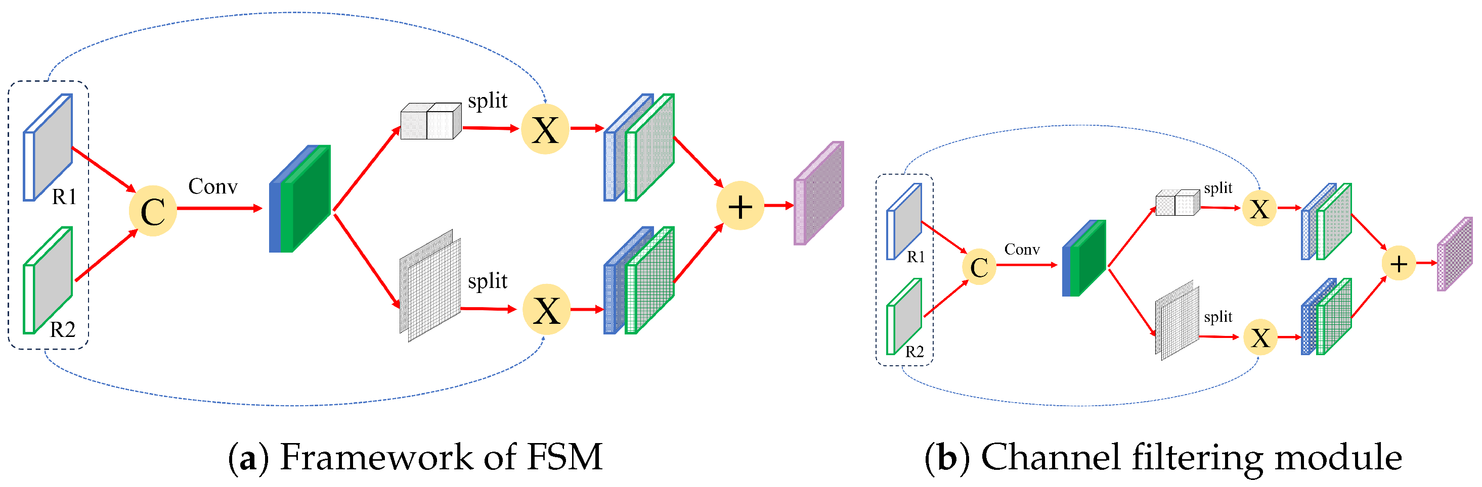
2.2.3. Feature Refinement Module

The effectiveness of object detection is improved by FPN as a result of fusing deep and shallow feature maps [36]. However, the large amount of redundant and conflicting information generated by the direct fusion of features at different scales is ignored, which limits the expression of the original multi-scale features. Therefore, FSM is proposed to filter conflicting information and prevent small object features from being submerged in the conflicting information. FSM modules are used to replace the Concat module of the original Neck layer (highlighted in purple in Figure 3). The overall structure of the FSM is shown in Figure 6.

From Figure 6, it can be seen that the FSM is mainly composed of two parallel branches, namely, a channel purification module and a spatial purification module. These are used to generate adaptive weights for the spatial and channel dimensions, which can then guide feature learning in more critical directions. The structure of the channel purification module is shown in Figure 5b. In order to obtain the channel attention map, the input feature map is compressed in the spatial dimension to aggregate spatial information that can represent the global features of the image. Adaptive average pooling and adaptive maximum pooling are combined to obtain more refined global image features. Here, $X_m$ is defined as the input of the mth $(m=\{1,2\left\}\right)$ layer of the FRM, $X_{(m,n)}$ is defined as the result of resizing from layer n to m, and $X_{k,x,y}^m$ is defined as the value of the mth feature map on the kth channel at position ($x,y$); thus, the output of the upper branch is

$$K_{x,y}^m=a^m·X_{x,y}^{(1,m)}+b^m·X_{x,y}^{(2,m)}$$

(1)

In the above formula, $K_{xy}^m$ represents the output vector of the mth layer at position $(x,y)$, while $a,b$ are channel adaptive weights with a size of 1 × 1 × 1, which are defined as follows:

$$a^m=\sigma \left[AP\left(F_1\right)+MP\left(F_1\right)\right],$$

(2)

$$b^m=\sigma \left[AP\left(F_2\right)+MP\left(F_2\right)\right].$$

(3)

where F is the feature generated through concatenation in Figure 5a, $\sigma$ represents a Sigmoid operation, and $AP$ and $MP$ represent the average pooling and maximum pooling operations, respectively. These two weights are then summed in the spatial dimension to generate channel-based adaptive weights through Sigmoid. The spatial filtering branch generates the weights of each position relative to the channel through Softmax, and the output of the lower-level branch is

$${\varphi }_{x,y}^m=\sum _{c=1}^2\sum _{c,x,y}\left({\mu }_{c,x,y}^m·X_{c,x,y}^{(1,m)}+v_{c,x,y}^m·X_{c,x,y}^{(2,m)}\right).$$

(4)

In Equation (3), x and y represent the spatial location of the feature map, k represents the channel of the input feature map, ${⌀}_{x,y}^m$ is the output feature vector at position $(x,y)$, and ${\mu }_{c,x,y}^m$ and $v_{c,x,y}^m$ denote the spatial attention weights with respect to the mth layer, where c denotes their channels; $\mu ,v$ are expressed as follows:

$${\mu }^m=Softmax\left(F_1\right),$$

(5)

$$v^m=Softmax\left(F_2\right).$$

(6)

The meaning of F in Formulas (5) and (6) is the same as in Formulas (2) and (3). Softmax is used to normalize the feature map in the channel direction to obtain the relative weights of different channels at the same position. Therefore, the total output of this module can be expressed as follows:

$$p_{x,y}^m={\varphi }_{x,y}^m+K_{x,y}^m.$$

(7)

In this way, the features of each layer of FPN are fused together under the guidance of adaptive weights and {$p1,p2,p3,p4$} are used as the final output of the entire network.

To verify the effectiveness of the FSM module, we replaced the original YOLOv5’s Concat with the FSM and compared them.

Table 2. Comparison of FSM and Concat under YOLOv5.

Adopt Module	mAP/%
Concat	83.1
FSM	87.9

shows the comparison results.

Table 2 shows the experimental results of YOLOv5 using Concat and FSM. As the table indicates, the network accuracy is improved by replacing Concat with the FSM module, resulting in a 4.8% increase in mAP. This demonstrates that the fusion of feature maps at different levels introduces conflicting and redundant information, and that the FSM module can suppress these conflicts to enhance the accuracy of peach blossom target detection.

2.2.4. K-Means++ Custom Anchor Box

The YOLOv5s algorithm uses K-means clustering to cluster the bounding boxes in the dataset and obtain the appropriate anchor box size. This method is simple and efficient; however, its initial clustering center selection is random, and the use of the Euclidean distance for distance measurement is easily affected by the size of the prediction box. Moreover, it is prone to falling into local optima and becoming unable to obtain global optima. To solve this problem, in this paper we use the K-means++ algorithm [37] in combination with the intersection over Union index (IoU) to set the anchor box of the dataset for improved randomness of the cluster center selection process. The influence of the size of the callout box can be avoided by using the IoU to establish distance metrics, which is more scientific and effective than using the Euclidean distance.

The specific steps for setting the anchor box followed in this paper are:

(1)

Randomly select a label box as the cluster center (Center1).

(2)

Calculate the shortest distance $D\left(i\right)$ between the other annotation boxes and all current cluster centers. Based on the shortest distance result, calculate the probability $p\left(i\right)$ of each annotation box being selected as the next cluster center and select the next cluster center based on this probability. Iterate the process until x cluster centers are selected.

(3)

After determining the cluster center, calculate the Distance$(i,j)$ between each annotation box and each cluster center, then assign them to the nearest cluster center. Based on this, calculate the mean of all annotation boxes contained in each cluster center in each dimension and update them to reflect the new cluster center. Iterate this process until the set number of iterations is reached or the cluster center no longer changes, then output x cluster center attributes. In the above process, the calculation formulas for the shortest distance $D\left(i\right)$, Distance$(i,j)$, and probability $p\left(i\right)$ are shown in Equations (8)–(10), respectively:

$$D\left(i\right)=min\left(\frac{1}{1+Io{U}_{(i,j)}}\right)$$

(8)

$$p\left(i\right)=\frac{D{\left(i\right)}^2}{\sum D{\left(i\right)}^2}$$

(9)

$$Distance(i,j)=\frac{1}{1+Io{U}_{(i,j)}}$$

(10)

Here, $i\in [1,N]$, where i represents the label box, N is the total number of label boxes in the dataset, j is the cluster center, with the value range $[1,X]$, and ${IoU}_{(i,j)}$ indicates the label box i and cluster IoU ratio of class center j.

The anchor frame sizes generated by the K-means++ clustering algorithm are shown in

Table 3. Anchor frame size.

Feature Map Scale	Anchor Box Size
	Anchor Box 1	Anchor Box 2	Anchor Box 3
80 × 80	[10, 13]	[16, 30]	[33, 23]
40 × 40	[30, 61]	[62, 45]	[59, 119]
20 × 20	[116, 90]	[156, 198]	[373, 326]

.

2.2.5. Improved Loss Function

In the YOLOv5s model, $CIoU$ is used as the detection frame regression loss function, considering the overlapping area, center distance, and aspect ratio of the predicted frame and the real frame in the bounding box regression, that is,

$$CIoU=IoU-\frac{{\rho }^2\left(b,b^{gt}\right)}{c^2}\alpha v.$$

(11)

Here, ${\rho }^2\left(b,b^{gt}\right)$ represents the Euclidean distance between the center point of the predicted frame and the center point of the real frame, C is the diagonal length of the smallest circumscribed rectangular frame that contains both the predicted frame and the real frame, and $\alpha v$ is the cost factor, which is used to make the regression more stable.

The calculation formula of CIoU-Loss is as follows:

$$L_{Clou}=1-CIoU.$$

(12)

The targets in the peach blossom dataset are characterized by a large number, small bounding boxes, and dense distribution. In areas with dense target distribution, the model may encounter issues with incorrect positioning. Considering that $CIoU$ does not take into account the direction mismatch between the required prediction box and the truth box, there may be situations where the degree of freedom of the prediction box is high, the convergence rate of the matching between the prediction box and the truth box is low, or the accuracy is low, negatively affecting the final prediction performance of the model for densely distributed areas. Integrating the directional information between the predicted box and the real box into the loss function is an effective method to avoid the aforementioned problems. Therefore, we use the $SIoU$ [38] loss function to replace the $CIoU$ in the original network. The $SIoU$ loss function consists of four cost functions, namely, the angle cost, distance cost, shape cost, and $IoU$ cost. The parameters used in the $SIoU$ loss function are shown in Figure 7.

It is possible to judge whether to minimize $\beta$ or $\alpha$ by whether the angle is greater than 45°; the calculation of the angle cost is shown in Formula (13):

$$\Lambda =1-2\times {sin}^2\left(arcsin\left(x\right)-\frac{\pi }{4}\right)$$

(13)

in

$$x=\frac{c_h}{\sigma }=sin\left(\alpha \right)$$

(14)

$$\sigma =\sqrt{{\left(b_{c_y,\mathrm{gt}}-b_{c_x}\right)}^2+{\left(b_{c_y,\mathrm{gt}}-b_{c_y}\right)}^2}$$

(15)

$$c_h=max\left(b_{c_y,\mathrm{gt}},b_{c_y}\right)-min\left(b_{c_y,\mathrm{gt}},b_{c_y}\right)$$

(16)

The distance cost represents the distance between the center point of the predicted frame and the real frame. Combined with the angle cost defined above, $SIoU$ redefines the distance cost, as shown in Formula (17):

$$\Delta =\sum _{t=x,y}\left(1-{\mathrm{e}}^{-\gamma {\rho }_t}\right)$$

(17)

in

$${\rho }_x={\left(\frac{b_{c_x,\mathrm{gt}}-b_{c_x}}{c_w}\right)}^2$$

(18)

$${\rho }_y={\left(\frac{b_{c_y,\mathrm{gt}}-b_{c_y}}{c_h}\right)}^2$$

(19)

$$\gamma =2-\Lambda$$

(20)

As $\alpha$ tends to 0, the contribution of the distance cost decreases substantially. On the contrary, when $\alpha$ is closer to $\pi$/4, the contribution of the distance cost is greater. As the angle increases, $\gamma$ is assigned a time-preferred distance value.

The definition of the shape cost $\Omega$ is shown in Equation (21):

$$\Omega =\sum _{t=w,h}{\left(1-{\mathrm{e}}^{-{\omega }_t}\right)}^{\theta }$$

(21)

in

$${\omega }_w=\frac{\left|w-w_{\mathrm{gt}}\right|}{max\left(w,w_{\mathrm{gt}}\right)}$$

(22)

$${\omega }_h=\frac{\left|h-h_{\mathrm{gt}}\right|}{max\left(h,h_{\mathrm{gt}}\right)}$$

(23)

where the value of $\theta$ defines how much attention is paid to the shape loss, which is set to 1 in this paper, which optimizes the aspect ratio of the shape, thereby restricting the free movement of the shape.

In summary, the final definition of the $SIoU$ loss function is shown in Equation (24).

$$L_{SIoU}=1-I_{IoU}+\frac{\Delta +\Omega }{2}$$

(24)

2.3. Experimental Environment and Parameter Settings

The configuration of the experimental platform is as follows: operating system, Linux 64-bit Ubuntu 18.04LTS; CPU, Intel ® core (TM) I9-9820X CPU @ 3.00 GHz; memory. 64G; GPU. Nvidia GeForce GTX 2080Ti; development environment, Python 3.8 (PyTorch 1.9.0, CUDA 10.1).The experimental model parameters are shown in

Table 4. Experimental model parameters.

Parameter Name	Value
Iterations	300 epochs
Learning rate	0.01
Momentum factor	0.973
Batch size	16
IOU threshold	0.5

.

2.4. Evaluation Index

This paper uses five common evaluation metrics for object detection models to evaluate model performance: precision (P), recall (R), average precision ($AP$), mean average precision ($mAP$), and frames per second ($FPS$).

Precision (P) is the proportion of correctly predicted targets among all targets, which can represent the relevance of the results. It describes the proportion of positive samples predicted as positive among all samples. The calculation formula is shown in Equation (25).

$$P=\frac{TP}{TP+FP}\times 100\%$$

(25)

$TP$ is the number of positive samples predicted correctly, while $FP$ is the number of positive samples predicted incorrectly, including detecting non-flower targets as flowers. Recall (R) is the ratio of the number of positive samples detected to the total number of actual positive samples, calculated as follows:

$$R=\frac{TP}{TP+FN}\times 100\%.$$

(26)

$FN$ is the number of misdetected positive samples, including cases where a target of one flower morphology is detected as another flower morphology category or not detected at all. Average precision ($AP$) is the area under the curve formed by P and R, calculated as follows:

$$AP={\int }_0^{1}P\left(R\right)\mathrm{d}R.$$

(27)

Mean average precision ($mAP$) is the main evaluation metric for object detection, measuring the overall performance of the network. It represents the mean of the $AP$ values for each category, and its measurement indicators are divided into two types: [email protected] and [email protected]:0.95. Unlike P and R, $mAP$ can evaluate the model’s merits and demerits independently, and its calculation formula is as follows:

$$mAP=\frac{\sum AP}{N}.$$

(28)

where N is the number of detection categories. In this paper, there are three categories, namely, bud, flower, and fallen flower; thus, N = 3. The average of the $AP$ values for all categories can be obtained as the $mAP$, which is generally used to evaluate the detection performance of the entire object detection network model.

The model inference speed (FPS) was obtained by taking the average of the detection time of 100 images using the server’s Nvidia GeForce GTX 2080Ti graphics card environment to detect the experimental image data, with a unit of frame/s.

3. Results

3.1. Impact of Improvement Methods on Model Performance

In order to analyze the impact of the improvement method proposed in this paper on the performance of the YOLOv5 algorithm, five sets of experiments were designed to analyze the results of different improved parts. Each experiment used the same training parameters, and the results of the impact of different methods on the model detection performance are shown in

Table 5. Comparison of models during the overall ablation test.

Small Object Detection Layer	CAM	FSM	K-Means++	SIOU	mAP/%	FPS
-	-	-	-	-	83.1	45.61
$\surd$	-	-	-	-	87.9	44.98
-	$\surd$	-	-	-	86.2	44.86
-	-	$\surd$	-	-	86.6	44.62
-	-	-	$\surd$	-	84.7	45.13
-	-	-	-	$\surd$	84.9	45.21
$\surd$	$\surd$	-	-	-	88.3	43.17
$\surd$	$\surd$	$\surd$	-	-	88.9	39.31
$\surd$	$\surd$	$\surd$	$\surd$	-	89.5	38.86
$\surd$	$\surd$	$\surd$	$\surd$	$\surd$	90.2	38.67

. Among them, “$\surd$” represents the corresponding improvement strategy used in the network model and “-” represents the corresponding improvement strategy not used in the network model.

According to the analysis in Table 5, although the FPS value decreased after adding different modules, the $mAP$ increased by 4.8% after adding a layer of feature maps specifically targeting small targets. This proves that the position information of shallow feature maps has a strong correlation with detecting small targets. The addition of feature maps specifically targeting small targets can further improve the network’s regression accuracy towards boundaries. The newly added CAM module improved accuracy by 3.1% compared to the original YOLOv5, proving that adding context information to FPN is beneficial for small target detection. Replacing Concat with the FSM module in YOLOv5 can improve the accuracy of the network, which is 3.5% lower than the previous $mAP$. It can be seen that feature map fusion at different levels brings about conflicting and redundant information. Through feature refinement in the FSM module, this conflicting information can be further suppressed, thereby improving the accuracy of peach blossom target detection. After adding the K-means++ algorithm, the $mAP$ increased by 1.6%, reflecting the ability of the K-means++ algorithm to avoid local optima and find global optima. After adding the $SIoU$ loss function, the loss of the prediction box was reduced, resulting in an improvement in regression accuracy and a 1.8% increase in $mAP$ value.

The training loss and validation loss curves in Figure 8 show that the loss value drops rapidly in the first 150 epochs of network training, with the loss curve gradually decreasing and tends to stability as the number of training rounds increases. The algorithm loss stabilizes when the number of epochs reaches roughly 300, when the model converges and no overfitting occurs during the training process.

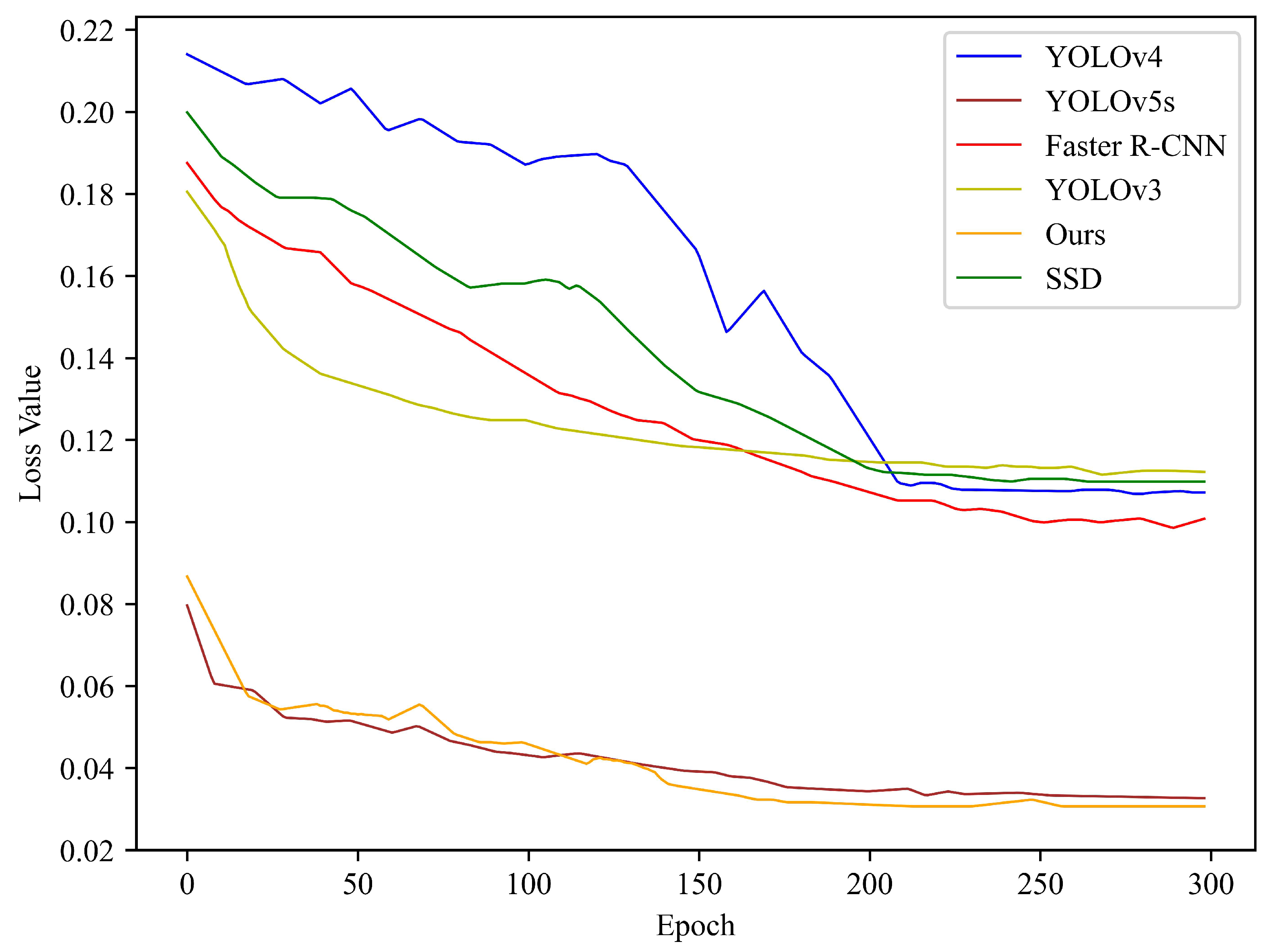
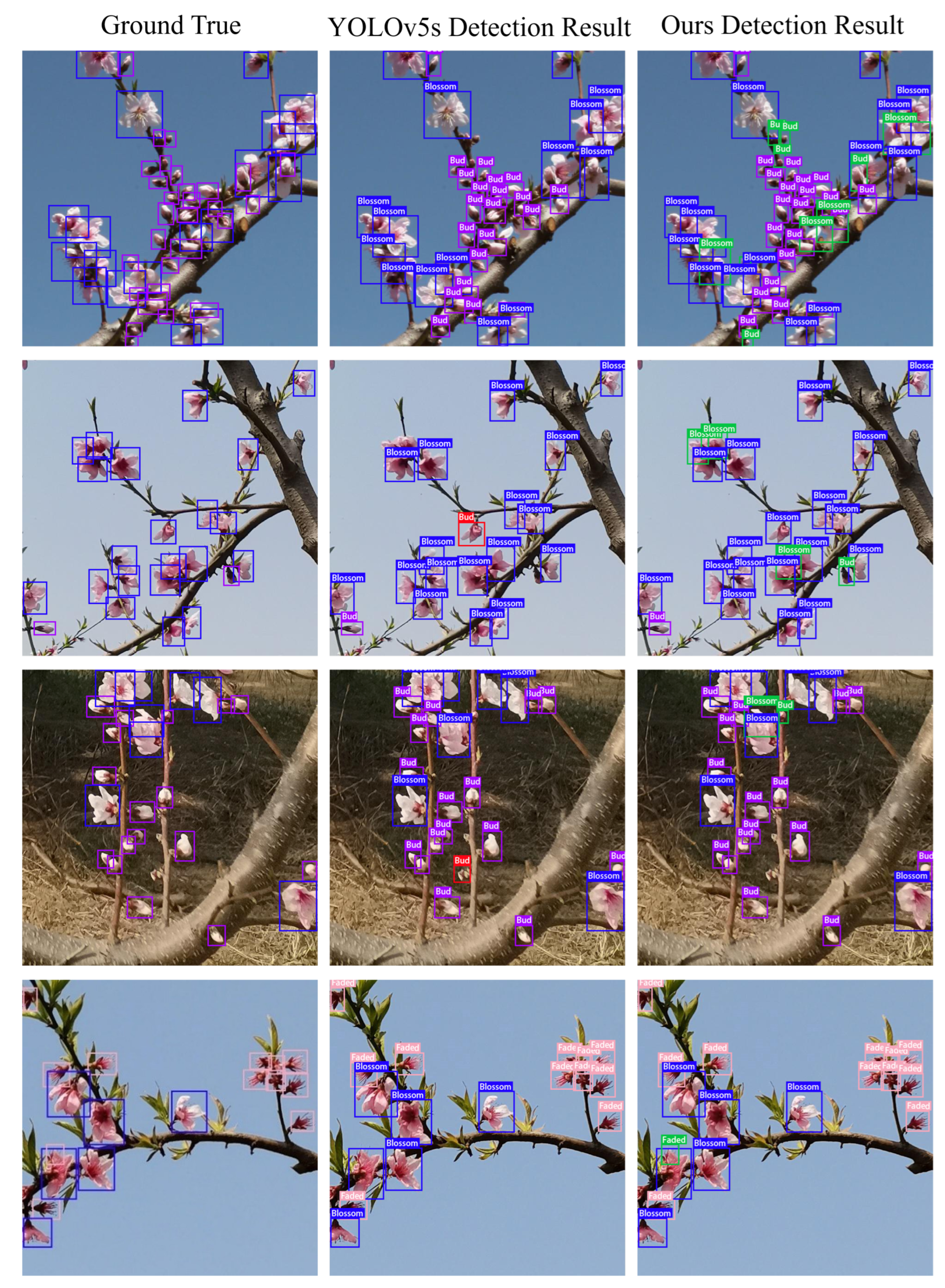
3.2. Performance Comparison of Mainstream Target Detection Models

To verify the detection performance of the improved algorithm proposed in this paper, the YOLOv5 algorithm was compared with the mainstream object detection models SSD, Faster RCNN, YOLOv3, and YOLOv4. The results are shown in

Table 6. Comparison between different object detection models.

Model	P/%	R/%	AP/% (IOU = 0.5)			mAP/%	FPS
			Bud	Blossom	Faded
SSD	71.2	88.7	74.3	72.4	77.6	74.5	32.26
Faster R-CNN	79.8	89.1	83.9	81.7	86.7	84.1	25.88
YOLOv3	82.5	81.2	78.0	79.2	88.5	81.9	31.12
YOLOv4	82.7	86.8	84.4	83.4	86.9	84.9	36.52
YOLOv5s	83.3	90.4	79.7	79.7	89.9	83.1	45.61
Our Method	90.1	93.2	87.5	89.8	93.3	90.2	38.67

.

As can be seen from Table 6, while the R values of SSD and Faster R-CNN are relatively high, their P values are below 80%. Overall, the P and R values of SSD, Faster R-CNN, YOLOv3, and YOLOv4 are significantly lower than those of YOLOv5s and our improved YOLOv5s algorithm. As shown in Table 6, YOLOv5s achieved good results on various indicators (P: 83.3%; R: 90.4%; mAP: 83.1%), and the model inference speed was 45.61 frame/s. Considering the high density of peach blossoms in a single image, the speed was within an acceptable range. The improved YOLOv5 algorithm increased the P value by 6.8 percentage points to 90.1% compared with the original YOLOv5 algorithm, while the R value increased by 2.8 percentage points to 93.2% compared with the original YOLOv5 algorithm and the mAP value reached 90.2%, which was 7.1 percentage points higher than the original YOLOv5 algorithm. By analyzing the AP values of the three types of peach blossom morphologies in the table, namely, buds, flowers, and fallen flowers, it can be concluded that our method has better detection performance for small objects, as the AP value of peach blossoms in the bud state is 7.8 percentage points higher than the original YOLOv5 algorithm when compared with the other mainstream object detection network models. By redesigning the feature fusion structure and multi-scale detection structure, the AP value of the flower detection targets was 10.1 percentage points higher than the original network model, and the experimental AP value for fallen flower detection surpassed both the original model and the mainstream object detection model. The frames per second of the improved model was 38.67, which was only 6.94 frame/s lower than the original model. While ensuring high-precision detection, the FPS of the model did not decrease significantly, and the detection speed showed an advantage compared with the mainstream models.

From the comparison of the post-training loss functions shown in Figure 9, it can be seen that the loss values of SSD, Faster R-CNN, YOLOv3, and YOLOv4 only decreases to around 0.1, while the loss values of YOLOv5s ultimately decreases to a lower level. The loss function proposed in this paper exhibits a smoother downward trend and has the lowest final loss value, indicating that the modified model is the most effective.

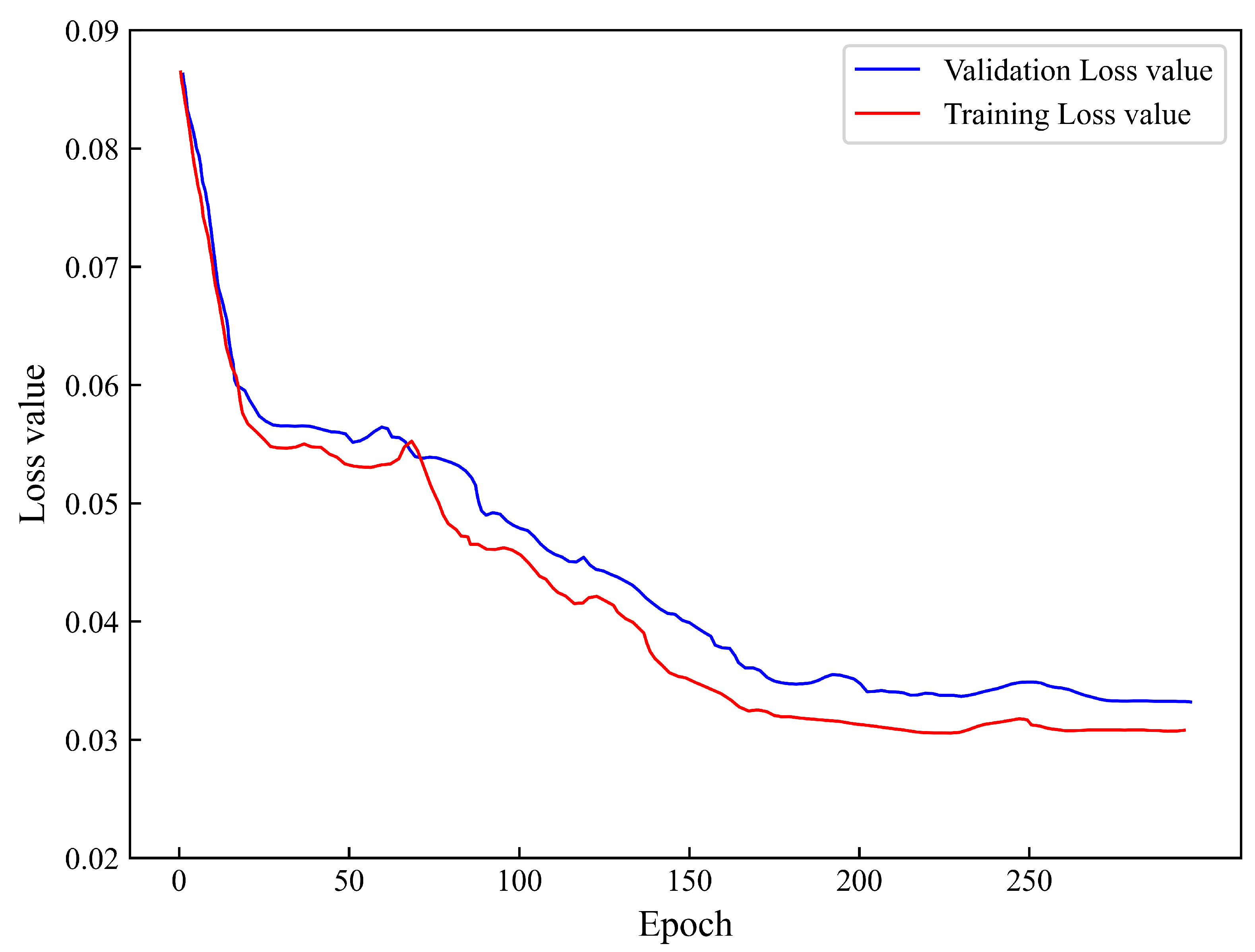
3.3. Comparison of Loss Values

Finally, object detection tests were performed on our model and the original YOLOv5s model. Part of the results are shown in Figure 10. The purple box represents the position of the flower bud label, the blue box represents the position of the flower label, the pink box represents the falling flower label, the green box represents targets that our model detected but YOLOv5s did not, and the red box represents targets detected by YOLOv5s in error. Overall, the model can solve missed and false detection problems, thereby improving inspection performance.

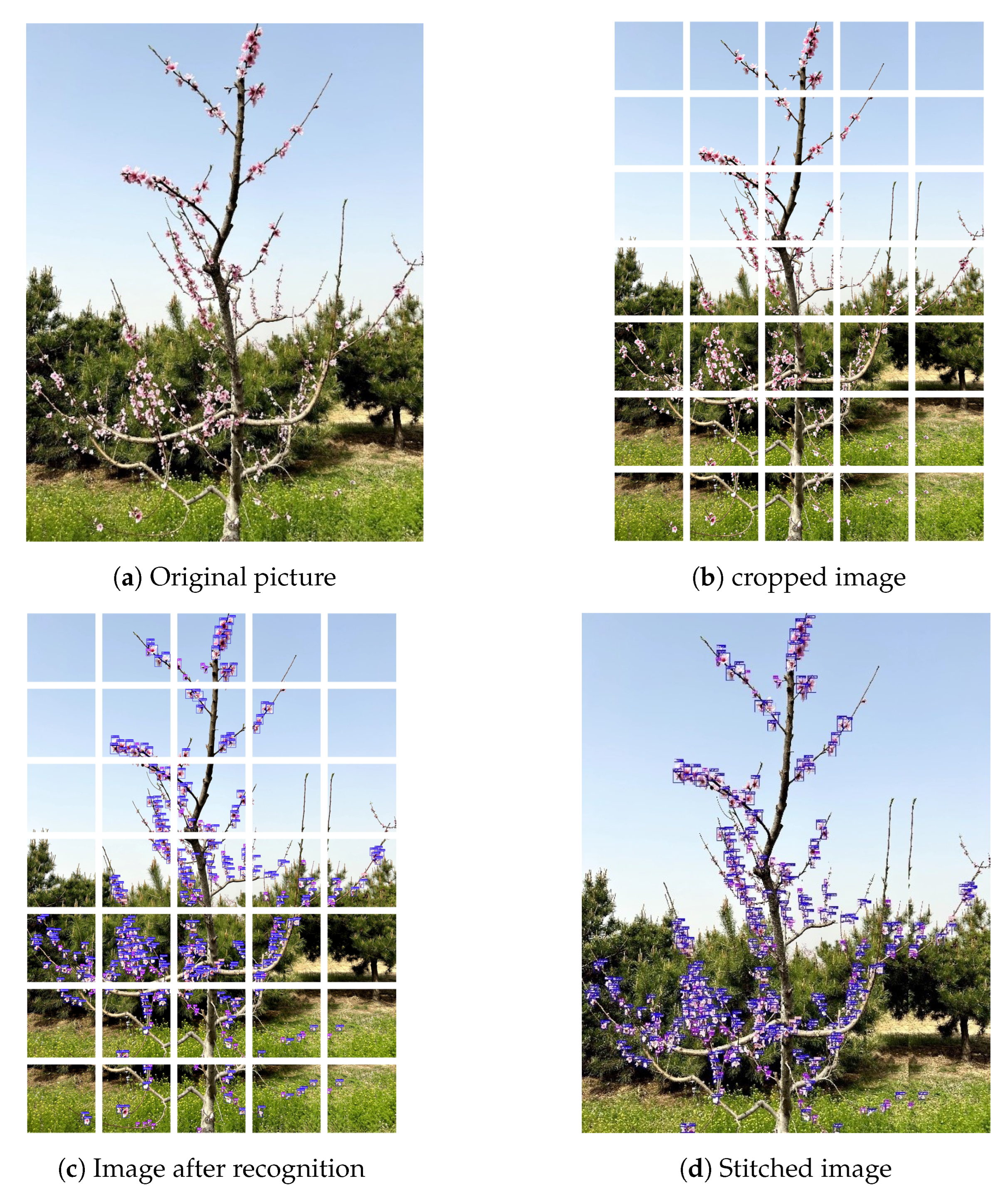
3.4. Model Application

First, the original image is cropped to fit the input image size of the model (640 × 640), then the cropped images are recognized separately, and finally the recognized images are concatenated to form the final recognition result. The identification steps are shown in Figure 11.

4. Discussion

The number of flowers on fruit trees is important for determining the thinning intensity and predicting the yield. Currently, the most common method for estimating the number of flowers is manual inspection, which is time-consuming, labor-intensive, and prone to errors. With the successful application of computer vision and deep learning in agriculture, researchers have started to use new technologies to obtain the flowering density of fruit trees. However, peach flowers have higher flowering density and smaller color variation among different types of flower morphologies compared with other fruit tree flowers. At present, there are few studies on peach flower recognition in the field of fruit tree flower recognition. The main methods are to use drones to aerially photograph a peach orchard during the flowering period to roughly identify the flower density [39] or to recognize single-type peach flowers [29]. There is a lack of methods able to recognize peach flowers with different growth morphologies. In this study, we use an improved YOLOv5s model to recognize three different peach flower morphologies and count the number of flowers.

Our experimental results show that the method proposed in this paper provides better AP values compared with current mainstream object detection algorithms for the recognition of three different peach blossom shapes, namely, buds, flowers, and falling flowers, with values of 87.5%, 89.8%, and 93.3%, respectively. The final mAP value for flower recognition reaches 90.2%, which can meet the requirements of monitoring peach tree flowering quantity.

The purpose of this study is to provide an effective method for obtaining more intuitive and accurate data sources for peach yield prediction and to lay a theoretical foundation for the development of thinning robots. Thinning is a highly labor-intensive task, and manual thinning makes it difficult to meet the thinning requirements of large orchards. However, the recognition performance of the model proposed in this study was only verified on the existing dataset, and further verification of peach blossoms from different regions is needed in the later stage to improve the generalization ability of the model. In the future, the model’s performance on embedded devices could be improved, and the network structure could be further optimized to achieve real-time detection and evaluation of peach blossom quantity on mobile devices when making thinning decisions.

5. Conclusions

In this paper, a flowering detection model is proposed for use on peach trees in natural environments. The test results show that our model has improved AP values compared with the original YOLOv5s model when identifying three different peach blossom shapes (buds, flowers, and falling flowers), by 7.8%, 10.1%, and 3.4%, respectively, while he final mAP value for peach blossom recognition is increased by 7.1%. Good results were achieved in detecting peach blossom volume, with higher performance than the general object detection model, potentially providing beneficial assistance for peach blossom period management.

References

1. Lakso, A.; Robinson, T. Principles of orchard systems management optimizing supply, demand and partitioning in apple trees. In Proceedings of the VI International Symposium on Integrated Canopy, Rootstock, Environmental Physiology in Orchard Systems 451, Wenatchee, WA, USA, Penticton, BC, Canada, 17 July 1996; pp. 405–416. [Google Scholar]
2. He, L.; Fang, W.; Zhao, G.; Wu, Z.; Fu, L.; Li, R.; Majeed, Y.; Dhupia, J. Fruit yield prediction and estimation in orchards: A state-of-the-art comprehensive review for both direct and indirect methods. Comput. Electron. Agric. 2022, 195, 106812. [Google Scholar] [CrossRef]
3. Jimenez, C.M.; Díaz, J.B.R. A statistical model to estimate potential yields in peach before bloom. J. Am. Soc. Hortic. Sci. 2003, 128, 297–301. [Google Scholar] [CrossRef]
4. Chanana, Y.; Kaur, B.; Kaundal, G.; Singh, S. Effect of flowers and fruit thinning on maturity, yield and quality in peach (Prunus persica Batsch). Indian J. Hortic. 1998, 55, 323–326. [Google Scholar]
5. Link, H. Significance of flower and fruit thinning on fruit quality. Plant Growth Regul. 2000, 31, 17–26. [Google Scholar] [CrossRef]
6. Dennis, F.J. The history of fruit thinning. Plant Growth Regul. 2000, 31, 1–16. [Google Scholar] [CrossRef]
7. Netsawang, P.; Damerow, L.; Lammers, P.S.; Kunz, A.; Blanke, M. Alternative approaches to chemical thinning for regulating crop load and alternate bearing in apple. Agronomy 2022, 13, 112. [Google Scholar] [CrossRef]
8. Kong, T.; Damerow, L.; Blanke, M. Influence on apple trees of selective mechanical thinning on stress-induced ethylene synthesis, yield, fruit quality, (fruit firmness, sugar, acidity, colour) and taste. Erwerbs-Obstbau 2009, 51, 39–53. [Google Scholar] [CrossRef]
9. Romano, A.; Torregrosa, A.; Balasch, S.; Ortiz, C. Laboratory device to assess the effect of mechanical thinning of flower buds, flowers and fruitlets related to fruitlet developing stage. Agronomy 2019, 9, 668. [Google Scholar] [CrossRef]
10. Kon, T.M.; Schupp, J.R.; Yoder, K.S.; Combs, L.D.; Schupp, M.A. Comparison of chemical blossom thinners using ‘Golden Delicious’ and ‘Gala’pollen tube growth models as timing aids. HortScience 2018, 53, 1143–1151. [Google Scholar] [CrossRef]
11. Penzel, M.; Pflanz, M.; Gebbers, R.; Zude-Sasse, M. Tree-adapted mechanical flower thinning prevents yield loss caused by over-thinning of trees with low flower set in apple. Eur. J. Hortic. Sci. 2021, 86, 88–98. [Google Scholar] [CrossRef]
12. Aggelopoulou, A.; Bochtis, D.; Fountas, S.; Swain, K.C.; Gemtos, T.; Nanos, G. Yield prediction in apple orchards based on image processing. Precis. Agric. 2011, 12, 448–456. [Google Scholar] [CrossRef]
13. Krikeb, O.; Alchanatis, V.; Crane, O.; Naor, A. Evaluation of apple flowering intensity using color image processing for tree specific chemical thinning. Adv. Anim. Biosci. 2017, 8, 466–470. [Google Scholar] [CrossRef]
14. Hočevar, M.; Širok, B.; Godeša, T.; Stopar, M. Flowering estimation in apple orchards by image analysis. Precis. Agric. 2014, 15, 466–478. [Google Scholar] [CrossRef]
15. Wang, Z.; Verma, B.; Walsh, K.B.; Subedi, P.; Koirala, A. Automated mango flowering assessment via refinement segmentation. In Proceedings of the 2016 International Conference on Image and Vision Computing New Zealand (IVCNZ), Palmerston North, New Zealand, 21–22 November 2016; IEEE: Piscataway, NJ, USA, 2016; pp. 1–6. [Google Scholar]
16. Wang, Z.; Underwood, J.; Walsh, K.B. Machine vision assessment of mango orchard flowering. Comput. Electron. Agric. 2018, 151, 501–511. [Google Scholar] [CrossRef]
17. Zhang, Z.; Luo, M.; Guo, S.; Liu, G.; Li, S.; Zhang, Y. Cherry fruit detection method in natural scene based on improved yolo v5. Trans. Chin. Soc. Agric. Mach. 2022, 53, 232–240. [Google Scholar]
18. Dias, P.A.; Tabb, A.; Medeiros, H. Apple flower detection using deep convolutional networks. Comput. Ind. 2018, 99, 17–28. [Google Scholar] [CrossRef]
19. Dias, P.A.; Tabb, A.; Medeiros, H. Multispecies fruit flower detection using a refined semantic segmentation network. IEEE Robot. Autom. Lett. 2018, 3, 3003–3010. [Google Scholar] [CrossRef]
20. Sun, K.; Wang, X.; Liu, S.; Liu, C. Apple, peach, and pear flower detection using semantic segmentation network and shape constraint level set. Comput. Electron. Agric. 2021, 185, 106150. [Google Scholar] [CrossRef]
21. Wang, X.A.; Tang, J.; Whitty, M. Side-view apple flower mapping using edge-based fully convolutional networks for variable rate chemical thinning. Comput. Electron. Agric. 2020, 178, 105673. [Google Scholar] [CrossRef]
22. Wang, X.A.; Tang, J.; Whitty, M. DeepPhenology: Estimation of apple flower phenology distributions based on deep learning. Comput. Electron. Agric. 2021, 185, 106123. [Google Scholar] [CrossRef]
23. Tian, Y.; Yang, G.; Wang, Z.; Wang, H.; Li, E.; Liang, Z. Apple detection during different growth stages in orchards using the improved yolo-v3 model. Comput. Electron. Agric. 2019, 157, 417–426. [Google Scholar] [CrossRef]
24. Farjon, G.; Krikeb, O.; Hillel, A.B.; Alchanatis, V. Detection and counting of flowers on apple trees for better chemical thinning decisions. Precis. Agric. 2020, 21, 503–521. [Google Scholar] [CrossRef]
25. Wu, D.; Lv, S.; Jiang, M.; Song, H. Using channel pruning-based yolo v4 deep learning algorithm for the real-time and accurate detection of apple flowers in natural environments. Comput. Electron. Agric. 2020, 178, 105742. [Google Scholar] [CrossRef]
26. Tian, Y.; Yang, G.; Wang, Z.; Li, E.; Liang, Z. Instance segmentation of apple flowers using the improved mask R–CNN model. Biosyst. Eng. 2020, 193, 264–278. [Google Scholar] [CrossRef]
27. Xia, Y.; Lei, X.; Herbst, A.; Lyu, X. Research on pear inflorescence recognition based on fusion attention mechanism 77 with yolov5. INMATEH-Agric. Eng. 2023, 69, 11–20. [Google Scholar] [CrossRef]
28. Shang, Y.; Zhang, Q.; Song, H. Application of deep learning using yolov5s to apple flower detection in natural scenes. Trans. Chin. Soc. Agric. Eng. 2022, 9, 222–229. [Google Scholar]
29. Tao, K.; Wang, A.; Shen, Y.; Lu, Z.; Peng, F.; Wei, X. Peach flower density detection based on an improved cnn incorporating attention mechanism and multi-scale feature fusion. Horticulturae 2022, 8, 904. [Google Scholar] [CrossRef]
30. Andriyanov, N.; Khasanshin, I.; Utkin, D.; Gataullin, T.; Ignar, S.; Shumaev, V.; Soloviev, V. Intelligent system for estimation of the spatial position of apples based on yolov3 and real sense depth camera D415. Symmetry 2022, 14, 148. [Google Scholar] [CrossRef]
31. Fan, S.; Liang, X.; Huang, W.; Zhang, V.J.; Pang, Q.; He, X.; Li, L.; Zhang, C. Real-time defects detection for apple sorting using NIR cameras with pruning-based yolov4 network. Comput. Electron. Agric. 2022, 193, 106715. [Google Scholar] [CrossRef]
32. Li, Y.; Wang, J.; Wu, H.; Yu, Y.; Sun, H.; Zhang, H. Detection of powdery mildew on strawberry leaves based on dac-yolov4 model. Comput. Electron. Agric. 2022, 202, 107418. [Google Scholar] [CrossRef]
33. Yan, B.; Fan, P.; Lei, X.; Liu, Z.; Yang, F. A real-time apple targets detection method for picking robot based on improved yolov5. Remote Sens. 2021, 13, 1619. [Google Scholar] [CrossRef]
34. Wang, Z.; Jin, L.; Wang, S.; Xu, H. Apple stem/calyx real-time recognition using yolo-v5 algorithm for fruit automatic loading system. Postharvest Biol. Technol. 2022, 185, 111808. [Google Scholar] [CrossRef]
35. Yu, F.; Koltun, V. Multi-scale context aggregation by dilated convolutions. arXiv 2015, arXiv:1511.07122. [Google Scholar]
36. Lin, T.Y.; Goyal, P.; Girshick, R.; He, K.; Dollár, P. Focal loss for dense object detection. In Proceedings of the IEEE International Conference on Computer Vision, Venice, Italy, 22–29 October 2017; pp. 2980–2988. [Google Scholar]
37. Arthur, D.; Vassilvitskii, S. How slow is the k-means method? In Proceedings of the Twenty-Second Annual Symposium on Computational Geometry, Sedona, AZ, USA, 5–7 June 2006; pp. 144–153. [Google Scholar]
38. Gevorgyan, Z. Siou loss: More powerful learning for bounding box regression. arXiv 2022, arXiv:2205.12740. [Google Scholar]
39. Horton, R.; Cano, E.; Bulanon, D.; Fallahi, E. Peach flower monitoring using aerial multispectral imaging. J. Imaging 2017, 3, 2. [Google Scholar] [CrossRef]
Figure 1. Example of the original image of the flower detection dataset used in this article.
Agriculture 14 00126 g001
Figure 2. Image labeling process.
Agriculture 14 00126 g002
Figure 3. Overall network structure. The CAM and FSM are the main components of the network; the CAM injects contextual information into the FPN, while the FSM filters conflicting information.
Agriculture 14 00126 g003
Figure 4. Structure of the CAM: features are processed by dilated convolution with rates of 1, 3, and 5, and the context information is obtained by fusing the features of different receptive fields.
Agriculture 14 00126 g004
Figure 5. Fusion method.
Agriculture 14 00126 g005
Figure 6. Proposed FSM.
Agriculture 14 00126 g006
Figure 7. Predicted and ground truth box vector angles.
Agriculture 14 00126 g007
Figure 8. Training and validation loss.
Agriculture 14 00126 g008
Figure 9. Comparison of training loss values between different target detection models.
Agriculture 14 00126 g009
Figure 10. Comparison of the method proposed in this paper with the partial detection results of YOLOv5s.
Agriculture 14 00126 g010
Figure 11. Peach blossom recognition steps.
Agriculture 14 00126 g011