Abstract
Food shortage issues affect more and more of the population globally as a consequence of the climate crisis, wars, and the COVID-19 pandemic. Increasing crop output has become one of the urgent priorities for many countries. To raise the productivity of the crop product, it is necessary to monitor and evaluate farmland soil quality by analyzing the physical and chemical properties of soil since the soil is the base to provide nutrition to the crop. As a result, soil analysis contributes greatly to maintaining the sustainability of soil in producing crops regularly. Recently, some agriculture researchers have started using machine learning approaches to conduct soil analysis, targeting the different soil analysis needs separately. The optimal method is to consider all those features (climate, soil chemicals, nutrition, and geolocations) based on the growing crops and production cycle for soil analysis. The contribution of this project is to combine soil analysis, including crop identification, irrigation recommendations, and fertilizer analysis, with data-driven machine learning models and to create an interactive user-friendly system (Soil Analysis System) by using real-time satellite data and remote sensor data. The system provides a more sustainable and efficient way to help farmers harvest with better usages of land, water, and fertilizer. According to our analysis results, this combined approach is promising and efficient for smart farming.
1. Introduction
Soil is a common material seen on Earth, and a natural material composed of solids (e.g., minerals and organic matter), liquids, and gases according to the definition by the Natural Resources Conservation Service (USDA, n.d.). The soil’s contribution in agriculture leads to the fact that the soil is highly coupled with human daily life. According to the Food and Agriculture Organization of the United Nations in 2015, approximately 95 percent of food is directly or indirectly produced from the soil, which raises the importance of soil since food is the essential energy and nutrition source for humans. The efficiency of food productivity draws more attention globally due to food supply and insecurity issues; smart agriculture helps us maintain soil health with more accurate nutrition to the crop. As a result, soil analysis via deploying smart agriculture techniques is crucial to maintaining the sustainability of soil in producing food and crops regularly.
Smart agriculture is an emerging field that introduces new technologies such as big data, IoT, satellites, and drones to help farmers optimize farming results. The benefits of smart agriculture include a reduction in manual labor, an increase in productivity, and a decrease in costs. While lack of unification is still one challenge for agriculture researchers and farmers, most agriculture research and applications focus on one specific area such as physical features, chemical features, or biological properties. Compared to previous research, (1) our research work proposes the vegetation indices calculated from satellite data, as well as various soil and fertilizer characteristics from public data resources. (2) Our work combines crop identification, irrigation system analysis, and fertilizer prediction into a whole analytical system. Outputs from crop identification modules are used as inputs for the irrigation system module, and then all the parameters flow into the fertilizer prediction module, making planting decisions and forecasts in one stage possible. (3) Our project provides a user-interactive system in soil analysis for people involved in agriculture fields and is user-friendly without requiring prior agriculture knowledge. The system is a web-based application. The backend is composed of machine learning models to perform the following tasks: crop analysis, irrigation recommendation, and fertilizer (nitrogen) recommendation. The frontend is a web interface for users to input their geolocation (e.g., GPS) of the area of interest and the analysis result will be outputted.
The organization of this paper is structured as follows. Section 2 is the review of the related work. Section 3 presents data engineering by introducing the raw data sources, the processing of data, the calculation of certain parameters, and the selection of parameters. Section 4 discusses machine learning model development, including the Random Forest, SVM, AdaBoost, Linear regression model, and the multilayer perceptron deep learning model. Section 5 shows the model evaluation where the best performance of the crop identification model is 78% in MLP; the R-squared score of the linear regression model for the irrigation system is 0.939; and the best accuracy score for the fertilizer recommendation model is 93.3% in MLP. Section 6 shows the system building and uses a case analysis. Section 7 displays the description of our visualization platform, an interactive map with the UI designed via Voila. Section 8 discusses and compares our system with other systems with similar functions. Section 9 concludes with three main achievements from the project.
2. Related Work
Table 1 shows the technical evolvement of crop identification. In the early stage (1969 to 1990) of crop identification, temporal-spectral data was used to calculate the vegetation index and to analyze the light of crop via building the crop growth and yield model. An alternative approach is to identify the lighter or darker tones of an image based on the field boundary and ground data. From 1991 to 2000, statistical analysis of the polarimetric multifrequency was getting popular, SAR data (the polarimetric C-, L-, and P-band from the AIRSAR system, as well as the X-band from the E-SAR system), sometimes combined with the pixel distributions of each agricultural plot, was used to calculate the crop’s wavelengths. Starting from 2000, vegetation indices such as NDVI, EVI, MSAVI, and NDWI were analyzed as spectral features in statistical approaches [1]. In the meantime, feature selection models were developed to improve the accuracy of the approach. From 2011 to now, various machine learning models, such as Random Forest and Support Vector Machine, have been deployed in crop identification by evaluating the spatiotemporal multispectral bands from satellites [2,3]. Moreover, deep learning models such as convolutional neural networks start to process the laudatory images with image feature capture [4,5].

Table 1.
The literature survey for crop identification.
In the consideration of the irrigation prediction system from Table 2, Mohammad Reza et al. [6] used a combination of decision tree algorithm and particle swarm optimization (PSO) for times series prediction for wastewater with an r-squared score of 95%. Istiak et al. [7] built an integrated irrigation network, by measuring the volumetric percentage of soil sample water content. The raw soil moisture data is collected by a moisture sensor. Shilpa [8] first classified the soil type under the KNN approach with humidity, temperature, and soil moisture as the parameters. Then, the authors calculated the water needed for the crop by using The Blaney−Criddle formula. Remilekun Sobayo et al. [9] created a CNN-based soil measurement by combining thermal images with the measurements of the farm area. The moisture level is valued by the soil temperature represented in it.
Table 2.
The literature survey for irrigation prediction.
Niko et al. [10] estimated the crop biomass and nitrogen content in the soil by extracting features from hyperspectral and RGB cameras. The methodology is based on Random Forest and simple linear regression. H. J. Escalante et al. [11] deployed a deep convolutional neural network to extract features from RGB images and then feed those features into predictive models. Diego et al. [12] also obtained the vegetation indices from remotely piloted aircraft images, which are applied to Random Forest machine learning methods to calculate the nitrogen content in coffee leaves. The global accuracy and the kappa coefficient are up to 0.91 and 0.86, respectively.
Fertilizer management is essential for land-use efficiency in Table 3. In recent years, machine learning and deep learning approaches have been conducted for most fertilizer prediction projects. Agarwal et al. [13] and Caturegli et al. [14] trained the models by analyzing crop images. Abhaya et al. [15] optimize the quantity of nitrogen fertilization considering the cost of labor and resources.
Table 3.
Literature Survey for Fertilizer Prediction.
3. Data Engineering
3.1. Data Collection
The datasets related to the project are mainly focused on two aspects: one is the on-the-ground task of crop identification and irrigation cycle system based on soil moisture analysis; another is the underground task of fertilizer recommendation based on soil nutrition analysis. Each objective needs different raw data and analytics tools. In Table 4, for the crop identification section, we built the models by utilizing satellite spectral data and land use maps; for the irrigation cycle system, the crop identification results are used as part of the inputs, combined with climate and soil data; for the fertilizer recommendation section, the crop types and soil data are used with nitrogen content data in the soil example.
Table 4.
Main tasks to develop models.
Currently, most of the soil and surrounding data come from public satellite data. The advantage of such data is easy to collect at a low cost, but the limitation is we cannot customize the data collection frequency. In the future, we plan to collect more specific agricultural data based on different farmlands, which need hyperspectral sensors, drone equipment, climate-based controllers, and LIBS sensors. In such a way, a personal workstation can connect to the soil analysis platform via the cloud.
3.1.1. Crop Identification: Land Use Map
The land use map from DWR gives the public access to statewide land and crop datasets for the last 30 years. It is a legislature-requested investigation into the aspects of agricultural land use and water needs. Most of the survey data are recorded into geographic information system (GIS) software by surveyors, who visited more than 95% of agricultural areas in the state and recorded the land usage [18].
We selected the dataset for San Joaquin County. Overall, there are 74,382 polygons delineated in the region, within which 34 objects are categorized. For example, acres, area_meter, class1, class2, class3, croptype1, croptype2, croptype3, irr_type1 [19]… We picked ‘Class1’ as the classification for land use, which is the first level of land use identification. The codes for the classification are all capital letters in Table 5.
Table 5.
Description of crop class on first level.
3.1.2. Irrigation Cycle: Precipitation
The definition of precipitation is the accumulated water amount that falls to the land surface. The amount of precipitation does not include the fog, dew, or other precipitation that has not fallen to the land ground before evaporating. The unit of the precipitation measurement is the meter and is assumed to be spread evenly to the land. In our crop water supply system, we use the precipitation parameter as the ‘crop water supply’ [20].
3.1.3. Irrigation Cycle: Evaporation
The unit of the evaporation measurement is the meter and is assumed to be spread evenly to the land [21]. We extracted evaporation bands from ERA5-Land, which is a reanalysis dataset by combining the model data with the observation data [22]. In Table 6, the evaporation parameter we used is the total evaporation band, which is the sum of evaporation from bare soil, open water surfaces, the canopy, vegetation transpiration, and snow evaporation.
Table 6.
Description of evaporation bands from ERA5-Lam.
3.1.4. Irrigation Cycle: Underground Water
Underground water is the water held by soil or rock under the land surface. Water is pulled through soil layers because of gravity, first reaching the upper layer zone of saturation called the ‘water table’, then going down to the deep layer called the ‘aquifer’ beneath the water table. Water in the aquifer moves slowly and recharges into land surfaces such as rivers, lakes, and oceans [23].
The underground water can be pumped out when the aquifer is shallow, and the water is able to move through the aquifer layer. The height of the water table is greatly influenced by precipitation patterns, climate, land surface changes, and human activities. We separated the soil above the groundwater into four layers, the shallowest layer is layer one and the deepest layer is layer four (Table 7). When layer one contains more water than layer four, the water table tends to become higher, meaning the excessive water is going to charge the water table and vice versa (Figure 1).
Table 7.
Description of soil layers.
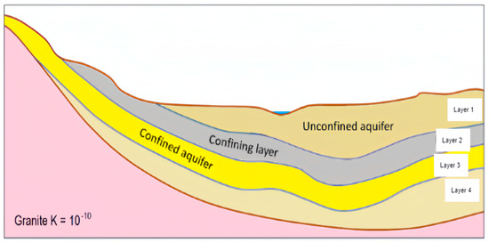
Figure 1.
Process of four soil layers (Earle, 2015).
3.1.5. Irrigation Cycle: Runoff
Runoff is a measurement of the ability to hold water in the soil; it is an effective indicator of flood or drought in the land (Table 8). The drainage of water from the land surface is called the surface runoff, while the drainage of water from the underground level is called the subsurface runoff [24]. Two subtype runoffs fall into the runoff category. The measurement of the unit is the depth in meters, which is assumed to be spread evenly across the grid area.
Table 8.
Description of Runoff.
3.1.6. Fertilizer Recommendation: Nitrogen
The Nitrogen prediction training data is taken directly from a research paper titled “Total nitrogen estimation in agricultural soils via aerial multispectral imaging and LIBS sensor” by Hossen et al. (2021) [25]. The dataset includes data taken from a drone-mounted sensor providing sensor data that includes features such as Red (Red band pixel value), NIR (Near Infra-Red Pixel Value), Green (Green Band Pixel Value), NDVI (Normalized Differential Vegetation Index), RH (Related Humidity), and Air Temperature. The dataset (Table 9) include the label in terms of actual Nitrogen content in the soil in ppm.
Table 9.
Soil Nitrogen content prediction dataset—training dataset.
3.2. Data Source and Pre-Processing
3.2.1. Step 1: For the Satellite Spectral Data, Vegetation Indices Are Calculated Based on Satellite Bands, with Assumed Adjustments and Coefficients
In Table 10, the bands used are shortwave bands from band 1 to band 8. B1 represents blue color with 0.45–0.52 µm, B2 represents green color with 0.52–0.60 µm, B3 represents red color with 0.63–0.69 µm, B4 represents near-infrared with 0.77–0.90 µm, B5 represents shortwave infrared with 1.55–1.75 µm, and B8 represents Panchromatic with 15 m resolution and 0.52–0.9 wavelength. Multiple vegetation indices are calculated based on referenced formulas [26], with some adjusted parameters and coefficients (Table 11).
Table 10.
Total bands based on satellite remote sensors.
Table 11.
Vegetation index formulas.
3.2.2. Step 2: For the Irrigation Module, Crop Water Requirement Is Calculated
For the crop water requirement (CWR), we combined three water outflow parameters for the final equation: the evaporation value, the total runoff value and the underground water amount. The negative value for evaporation means the water flows out of the land surface, and the positive value for runoff represents the water running away from the soil layer. “ET_runoff” presents the sum-up of evaporation and runoff. Then, we added up the soil water values from the 4th layer to the 1st layer to get the total ‘Underground Water’ parameter.
3.2.3. Step 3: For the Fertilizer Recommendation, the Criteria to Bucket the Data Are Defined and Continuous Elements Are Separated into Different Buckets [7]
As mentioned in the data preprocessing section, the label available in the training dataset is a continuous value and hence is not suited for classification models. Hence, as part of the data transformation, we converted the continuous variables to discrete values. The discrete values were grouped into 3 ‘Tier’ ranges. Low-1 (0–500 ppm), Medium-2 (501–1000 ppm), and High-3 (>=≥1001 ppm). The processed dataset is shown Figure 2.
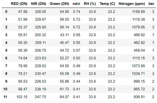
Figure 2.
Transformed data sample for fertilizer recommendation model.
3.3. Data Parameter Selection and Analysis
To analyze the difference in vegetation indices behavior, we collected the spectral reflectance based on Landsat 8 collections for different crop types.
Figure 3 presents the linearity relationships between vegetation indices and near-infrared band (NIR), with the reason that NIR is a good indicator of foliage cover and crop growth. The more leaf area variation depicted by the NIR index, the greener the pigment shows. From the picture we can see that MSR is the most sensitive vegetation index to the variation of NIR, ranging from 0.2 to 2.0 when the NIR increased from 0.2 to 0.6. MCARI has the weakest correlation with NIR, keeping flat around 0.0 no matter how NIR changed. TVI also did not show an apparent relationship with NIR and became saturated at around 0.5 with the changes in NIR. The sensitivities of other vegetation indices sit among MSR and MCARI, they behaved quite similarly with an average slope of 0.6.
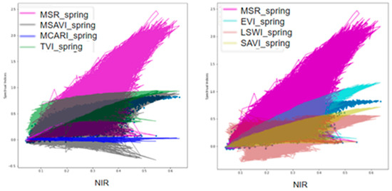
Figure 3.
Relationship between vegetation indices and NIR.
In the training features, we removed MCARI and TVI since they show almost no correlation with the crop cover. In contrast, we selected MSR, EVI, LSWI, SAVI, and MSAVI as the features for machine learning models.
In the prepared irrigation dataset, we select 8 input variables: CWS, ET_runoff, underground water, CWR, heat flux, skin temperature, wind, and NDVI. It is noted from Figure 4 that CWS has a linear relationship with underground water, CWR, ET_runoff, and skin temperature. So, we will first try to build linear regression models with regularizations among CWS and other features.
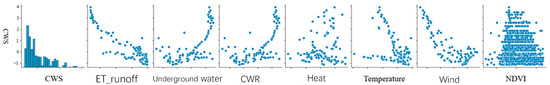
Figure 4.
Correlation among input features of the irrigation dataset.
3.4. Data Preparation and Segregation
We divided the dataset into training and testing datasets with 80% for training and 20% for testing (Table 12). Since the label output is an abnormal distribution, we stratified the training and testing dataset according to the weights of crop amounts. There are 17,561 rows of data, 9 input features, and 1 label in the crop identification dataset. For the irrigation cycle dataset, there are more than 2000 rows for training, 6 input features, and 1 label. For the fertilizer recommendation, we select 14,096 rows of data for the training dataset, 5 input features, and 1 label.
Table 12.
Descriptions of Datasets.
4. Model Development
4.1. Random Forest
Random Forest is one of the most widely used Classification algorithms, which uses the Ensemble Learning Technique [32]. One of the main advantages of Random Forest is that it creates many decision trees on the input subset data and combines all the outputs into a final prediction as shown in Figure 5 [33]. Random Forest methods are less prone to overfitting problems and tend to have better accuracy than other classification methods. For the crop identification module [34], we ran the randomized search on the Random Forest model with 5 cross-validations to find the optimized parameters. The best parameters are 100 estimators, 2 minimal samples split, 100 maximum depths, and entropy as the criterion.
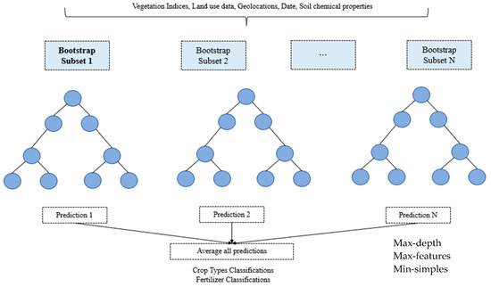
Figure 5.
Model of Random Forest.
4.2. SVM
Support vector machines are a supervised learning approach for classification. With the kernels function defined as polynomials, SVM is also an efficient nonlinear classifier of high-dimensional space. There are two primal parameters tuning the SVM, one is the C parameter to soften the margin, and another is the gamma parameter to define the radius influence. For the crop identification module, grid search was first deployed to find the optimal estimators. The best parameters are ‘kernel = rbf’, ‘gamma = 0.25’, ‘C = 200’, and ‘cross validation = 5’.
4.3. AdaBoost
AdaBoost is an ensemble method to convert weak learners into strong learners. The mistakes from the previous stump are considered for the next one. The weights of different stumps are dependent on error calculations, the incorrect data predicted in the former stump will be given more weight in the next stump-making process. For the crop identification module, the following parameters are tuned: base estimator, number of estimators, learning rate, and depth of the decision tree. The best parameters are ‘base_estimator_max_depth = 4, ‘learning_rate= 0.1’, and ‘n_estimators = 100’.
4.4. Linear Regression Model
A simple regression model is formed with one input (X) to estimate the output (Y). In the higher dimension linear regression model, there are multiple inputs (X) in the equation and the line is called a hyper-plane. We deployed a linear regression model and a polynomial regression model with multiple regularizations. For the irrigation cycle module, the parameters used in polynomial regression models are ‘alpha = 0.1’, ‘alpha = 0.01’, ‘alpha = 0.0001’, and ‘degree = 2’. Moreover, we put different combinations of inputs to evaluate the result of y. By using statistical approaches such as mean squared error (MSE), root mean squared error (RMSE), mean absolute error (MAE), and R-squared, we seek optimized accuracy.
Y = B0 + B1x + B2x + B3xy
4.5. Multilayer Perceptron (MLP)
Multilayer perceptron (MLP) is a kind of feed-forward neural network consisting of an input layer, output layer, and hidden layer. Each layer is fully connected with other layers. MLPs are widely used to solve supervised machine learning problems. The weights and bias during the training can be adjusted to minimize the classification error [35]. For the crop identification module shown in Figure 6, there are three dense layers (each with 40 neurons) following a ‘relu’ activation function, and then a regulatory layer with a 10% dropout is used before the output layer. For the fertilizer recommendation module, it shares the same MLP structure but with different inputs.
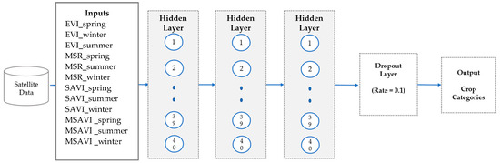
Figure 6.
Model of Multilayer Perceptron.
5. Model Evaluation
In Table 13, there are five machine learning models built for the crop identification module. Only the AdaBoost model has the overfitting issue as the training size grows. In Figure 7, the learning curve of SVM goes down, apparently, and the gap between the training curve and validation curve shrinks since more data samples are put in the model. The deep learning model performed the best with 78% accuracy, whose loss dropped down quickly before the first 20 epochs and stayed saturated at around 0.75. The model accuracy also changed evidently before the first 20 epochs and improved slowly to 0.78 after 300 epochs. Hence, the MLP model is selected as the candidate model for the system.
Table 13.
Crop identification evaluation metrics.
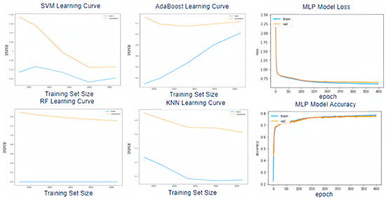
Figure 7.
Learning curves for crop identification models.
Based on the irrigation cycle evaluation metrics shown in Table 14, there are three linear regression models built to predict the crop water supply. One is the original linear regression, the second is the linear regression with Lasso regularization, and the third is polynomial regression. Gridsearch is conducted to all the hyperparameters tuning alpha = 0.1, 0.01, 0.001; degree = 2. The best R-squared score is 0.939 from polynomial regression, and the best testing score is 0.9364 from polynomial regression.
Table 14.
Irrigation cycle evaluation metrics.
Figure 8 shows the different irrigation levels across the country. The more left side of the color bar (dark blue), the drier that area is. On the west coast (lower right picture), a yellow and pink panel represents a moist land area. In the middle part of the country (upper left picture), the panel in dark blue means the soil of that region is extremely dry. When we talked about the east coast, no matter whether upper east or lower east, neither of the areas is good at retaining moisture in the soil.
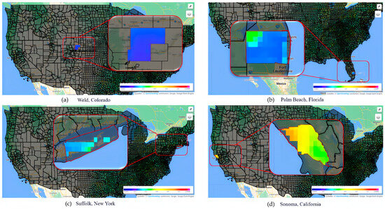
Figure 8.
Color panels for the crop water supply prediction model: (a) middle America; (b) lower east coast; (c) upper east coast; and (d) west coast.
For the fertilizer recommendation module shown in Table 15, five machine learning models were built to find the optimal results. The multilayer perceptron deep learning model performed the best, with an accuracy score of 93.3% after 100 epochs. So, we selected the MLP model as our final deployed model for the fertilizer recommendation system. We classified the continuous outputs into three bins [36]: blue means less fertilizer, yellow means neutral fertilizer, and green means rich fertilizer. From Figure 9, we can see that the first selected area has enough fertilizer in the soil, and the second selected area in dark green represents sufficient nutrients [37].
Table 15.
Fertilizer recommendation evaluation metrics.
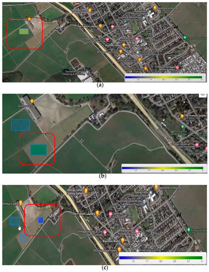
Figure 9.
Color panels for fertilizer recommendation prediction model: (a) yellow means neutral fertilizer; (b) green means rich fertilizer; and (c) blue means less fertilizer.
6. Data Analytics System
6.1. System Requirements Analysis
6.1.1. System Boundary and Use Cases
Our use cases mainly happen in three environments: personal workstations, research labs, and agriculture business companies. The corresponding users of our system (Soil Analysis System) are farmers who plant and study in their personal workstations, scientists in research labs, and technicians from agriculture business companies. Figure 10 illustrates three different kinds of scenarios for each user and the use case. The scenario can be summarized as follows:
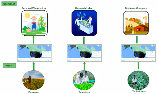
Figure 10.
Soil analysis system boundary and use cases.
A farm worker (e.g., farmer, scientist, or technician) performs the assessment of the interested farmland using this system before determining the cultivation plan. The system returns the analysis report listing crop identification, irrigation supply, and fertilizer recommendation, given the selected farmland. The system is a web application and would be run in the farm worker’s workspace (e.g., personal workstation, research lab, or inside an agriculture business company). The detailed analysis of farmlands is essential and vital for every cultivation since different farmlands should be taken care of differently, and it leads to more productive, efficient, and ecological cultivation [38].
6.1.2. System High-Level Data Analytics
The high-level data analytics of the project is made up of three tiers: reporting, insights, and prediction. At the reporting level, we construct a crop identification platform [39], which is able to recognize different types of crops based on the sensors’ bands. Each crop has its special vegetation indices features, we trained the machine learning models to learn the general disciplines among diversified crops and try to tell the type of crop.
At the insights level, we created our own formula to analyze irrigation situations based on the surface water and underground water data. The calculation of surface water is dealing with the precipitation, irrigation, and temperature of the land. The calculation of the underground water includes the different layers of water level (four layers).
In the prediction level, we forecast the fertilizer usage of one specific farmland for the next season combined with the results from the first crop identification part and the second irrigation recommendation part. Additionally, the nutrition data about the soil (NPK), collected from the sensors, is critical to the prediction process. With respect to the use of the data, deep learning models will be deployed to recommend fertilizer usage.
6.2. System Design
6.2.1. System Architecture and Infrastructure
Figure 11 shows our system architecture of this project, which has a three-layer architecture: a user interface layer, a machine learning layer, and a data storage layer. The user interface layer runs on a web browser as the frontend. The user (e.g., farmer, scientist, or technician) can interact with our system via the web application. Via the user interface, the user can specify the farmland information by entering a geographical location or selecting the area of interest from the visualized map.
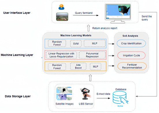
Figure 11.
Full stack soil analysis system architecture.
The data storage layer consists of two parts: a database access to the satellite data from Google Earth Engine and one database with LIBS sensor data (McMillan, 2018). After our frontend receives the query of the farmland, the frontend then sends the query to the data storage layer. According to the information, the backend extracts the corresponding data, including both satellite data and sensor data, and sends them to our trained machine learning model.
The machine learning layer consists of three modules: crop identification, irrigation supply prediction, and fertilizer recommendation. In the first module, Random Forest, SVM and MLP are deployed in identifying the crop. The irrigation cycle prediction module is performed by using linear regression with lasso regularization and polynomial regression. The fertilizer recommendation is mainly conducted by Random Forest, SVM, and MLP. After three modules complete our comprehensive soil analysis, the report of the soil analysis is returned and displayed on the user interface.
6.2.2. Inputs, Outputs, and Data Flow
The data flow shown in Figure 12 shows that the whole system includes four parts: user input, agriculture inputs, model, and module outputs. The outputs connect the three modules and support the results. In the first input part, users give the area of interest, such as latitude and longitude coordinates, to settle on the specific location they want to focus on. Then, the system will retrieve the selected area from the global satellite dataset in Google Earth Engine. Based on the algorithm to retrieve data, the system will pull the spectral bands from the dataset. The output from the crop identification model flows into the second module as the inputs, combined with climate data and surrounding water data. The chemical prediction model will be fed with soil moisture data from the second module and spectral band data from the first module.
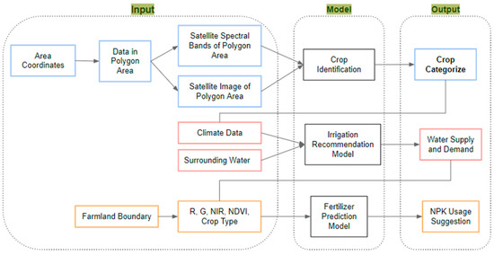
Figure 12.
Inputs and outputs of soil analysis system requirements.
7. Visualization Platform
Our visualization platform describes the real-time soil conditions for the United States based on the Landsat 8 dataset. We offer a variety of commonly used vegetation indices, with which we can find the crop classification for certain farmland areas. Moreover, the platform enables the users to check the water demand for irrigation and fertilizer usage recommendations. Our goal is to help users monitor cropland vegetation conditions and predict the soil condition. The observable time ranges from 1984 to 2022; more than 20 years of observation data can analyze the geospatial time series and detect changes in many research fields [40] (Figure 13).
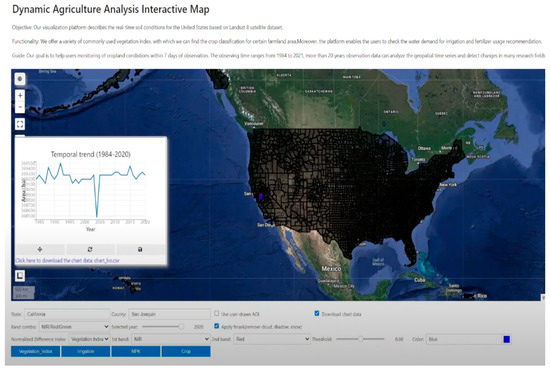
Figure 13.
UI of Interactive Crop Analysis Map.
At the top left of the UI, there is a weight to select the location or data that the user is interested in. There are three ways to search the location, the first way is the ‘name/address’ function searching by place name or address such as Paris, the second way is the ‘lat-lon’ function searching by ‘lat-lon’ such as 40, −100, the third way is ‘data’ function searching by GEE data catalog by keywords such as elevation. The map can zoom in to the county level and click certain counties in the USA such as San Joaquin (Figure 14). Once the county is selected, the user can select whether to download the chart data to check the statistics. All the downloaded data is stored as CSV files, and the line chart can also be saved in the client’s local server (Figure 15).
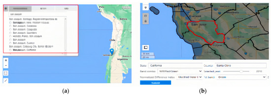
Figure 14.
(a) Location selection widget; (b) county-level location selection.
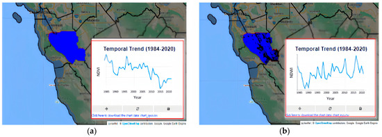
Figure 15.
(a) Chart data for NDVI from 1985 to 2020; (b) chart Data for NDWI from 1985 to 2020.
The moisture level is presented by a color bar. Blue means the area is dry and red means the area is moist. The colors between blue and red in the color bar present the middle level of soil humidity. From Figure 16, we can say that the soil of the San Joaquin area is relatively moist, with a yellow and pink pallet. The users can check the soil moisture level for other counties by clicking the polygon of that county.
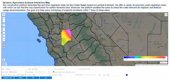
Figure 16.
UI of Interactive Irrigation Analysis Map.
The fertilizer condition is classified into three categories, less fertilizer (blue), neutral fertilizer (yellow), and more fertilizer (green) in Figure 17. The selection area can be focused on one specific farmland, by drawing the area of interest (AOI).
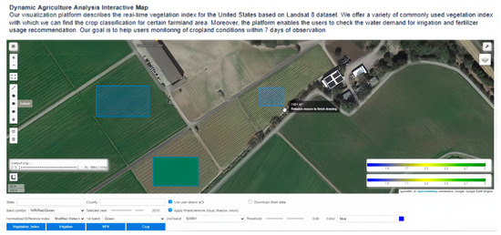
Figure 17.
UI of Interactive Fertilizer Analysis Map.
8. Discussion
8.1. Soil Nutrient Analysis Incorporates the Features from Crop Spectral Data and Soil Biological Data
We have assembled a set of attributes for a soil health detection system, based on three attributes: crop characters, soil biological status, and soil nutrient status. These features provide data to be used in our final platform for the users to assess the soil health information. For the crop identification module, five vegetation indices calculated from remote sensing data, MSR, EVI, LSWI, SAVI, and MSAVI, are used in the final categorized machine learning models, of which MLP performed the best with 7 selected crop types. For the irrigation supply module, the linear regression model is applied with 6 input features, and the ‘evaporation and runoff’ feature is the most correlated one with a 0.68 coefficient factor, wind feature is the second with a 0.4 coefficient factor. Since all the p-values are less than 0.05, we kept all the input features in the final linear regression model. For the fertilizer module, RH and temperature are added into consideration as the input features along with the spectral data and biological data.
8.2. Creative Soil Analysis Platform Confusion
The traditional way to collect soil data is field observation via crop reports or sensors, which is time-consuming and has high costs. The modern way is to measure passive land surface microwave emission and radar backscatter, which is more robust and reliable. Most soil analysis systems combine those data sources with geospatial data to visualize and monitor soil status.
Our nutrient analysis approach uses the result from the crop identification module and irrigation module, providing an efficient way to utilize physical and biological soil data with cost efficiency. Our platform is a creative system that combines multiple soil analysis steps into one work, benefiting small-scale farmers specifically. In the future, we will deploy customized research results based on local drone and sensor data.
8.3. Farmland Biological and Chemical Features Are Not Dependent on the Farmland Geolocation
Our soil analysis system incorporates satellite information, which takes the longitude and latitude of the field as inputs to assist the users in monitoring their interested field even if they work remotely. It benefits the remote research happening in companies or labs for soil analysis. According to the changes in the color bars from the interactive map, we found that the west coast of America is moister than the east coast, despite both lands being located on the coast. The fertilizer situation is also not directly related to the geolocation but is more dependent on the single farmland environment. Even the nearby lands could have completely different fertilizer levels. No IoT or pH sensors are used to collect agriculture chemicals.
We will try to build a data pipeline, which can update data automatically. Soil health analysis is routinely challenged by the dynamic and complicated nature of environmental changes. A dynamic modelling system can demonstrate continuous value across the farmlands to help users understand and predict the dynamic environment and behavior in support of decision making.
9. Conclusions
Our integrated soil analysis approach has three main contributions as follows:
The first contribution is to combine soil health analysis with crop type, land water, and fertilizer usage. The precision of the crop type classification is dependent on the spectral bands data, then the crop type information will be infused into the irrigation prediction system. All these crop and land water data are the inputs for the fertilizer analysis. In such a way, we minimize the number of parameters coming from outside resources and use our own dataset via cyclic utilization.
The second main contribution is the irrigation calculation. The theory behind the calculation comes from the natural hydrologic system, which is a cyclic water environment of the earth including precipitation, evaporation, transpiration, streamflow, and underground water. We calculated the crop water supply (CWS) against the crop water requirement (CWR). Both parameters consist of several separate data sources. For the crop water supply (CWS), precipitation and underground water pumping are included. For the crop water requirement (CWR), evaporation and runoff are considered.
The third main contribution is that the interactive map platform we built can check the crop and soil information for farmland users. They not only can click the functional buttons that we built in, but also customize their own area of interest to find one certain farmland’s situation. Moreover, the users can download the data, which are integrated from multiple public data sources via our system, saving the user’s time with no need to search for the data separately online.
Currently, our application only takes the geolocation data of the regions in San Joaquin County. In the future, we want to expand our application nationwide. Moreover, we would deploy crop analysis on every single crop, providing more detailed end-to-end analytical reports for the users.
Author Contributions
Conceptualization: Y.H., R.S. and C.N.; Methodology: Y.H., R.S. and C.N.; Software: Y.H., R.S. and C.N.; Validation: Y.H., R.S. and C.N.; Formal Analysis: Y.H., R.S. and C.N.; Resources: Y.H., R.S. and C.N.; Data curation: Y.H., R.S. and C.N.; Writing—original draft preparation: Y.H., R.S. and C.N.; Writing—review and editing: Y.H.; Visualization: Y.H., R.S. and C.N.; Supervision: J.G. and J.W.; Project administration: Y.H., J.G. and S.C.; Funding Acquisition: S.C. All authors have read and agreed to the published version of the manuscript.
Funding
This research was partially funded by the U.S. Department of Commerce, National Oceanic and Atmospheric Administration, Educational Partnership Program under Agreement No. NA22SEC4810015. The APC was funded by Dr. Sen Chiao. Professor NOAA Center for Atmospheric Sciences and Meteorology, Howard University.
Institutional Review Board Statement
Not applicable.
Data Availability Statement
The data presented in this study are openly available via the links provided in the Reference section.
Conflicts of Interest
The authors declare no conflict of interest.
References
- An, Q.; Gao, W.; Yang, B. Research on Feature Selection Method Oriented to Crop Identification Using Remote Sensing Image Classification. In Proceedings of the Sixth International Conference on Fuzzy Systems and Knowledge Discovery, Tianjin, China, 14–16 August 2009. [Google Scholar]
- Singh, J.; Mahapatra, A.; Basu, S.; Banerjee, B. Assessment of Sentinel-1 and Sentinel-2 Satellite Imagery for Crop Classification in Indian Region During Kharif and Rabi Crop Cycles. In Proceedings of the IEEE International Geoscience and Remote Sensing Symposium, Yokohama, Japan, 28 July–2 August 2019. [Google Scholar]
- Saxena, V.; Dwivedi, R.K.; Kumar, A. Analysis of Machine Learning Algorithms for Crop Mapping on Satellite Image Data. In Proceedings of the 10th International Conference on System Modeling & Advancement in Research Trends (SMART), Moradabad, India, 10–11 December 2021. [Google Scholar]
- Chen, K.-H.; Lin, C.-C.; Chen, C.-H. Crop Classification on Deep Learning. In Proceedings of the IET International Conference on Engineering Technologies and Applications (IET-ICETA), Changhua, Taiwan, 14–16 October 2022. [Google Scholar]
- Puspaningrum, A.; Sumarudin, A.; Putra, W.P. Irrigation Prediction using Machine Learning in Precision Agriculture. In Proceedings of the 5th International Conference of Computer and Informatics Engineering (IC2IE), Jakarta, Indonesia, 13–14 September 2022. [Google Scholar]
- Mohebbian, M.; Vedaei, S.S.; Bahar, A.N. Times Series Prediction used in Treating Municipal Wastewater for Plant Irrigation. In Proceedings of the 2019 IEEE Canadian Conference of Electrical and Computer Engineering (CCECE), Edmonton, AB, Canada, 5–8 May 2019. [Google Scholar]
- Mahmud, I.; Nafi, N.A. An approach of cost-effective automatic irrigation and soil testing system. In Proceedings of the 2020 Emerging Technology in Computing, Communication and Electronics (ETCCE), Dhaka, Bangladesh, 21–22 December 2020. [Google Scholar]
- Chandra, S.; Bhilare, S.; Asgekar, M.; Ramya, R.B. Crop Water Requirement Prediction in Automated Drip Irrigation System using ML and IoT. In Proceedings of the 4th Biennial International Conference on Nascent Technologies in Engineering (ICNTE), NaviMumbai, India, 15–16 January 2021. [Google Scholar]
- Sobayo, R.; Wu, H.-H.; Ray, R. Integration of Convolutional Neural Network and Thermal Images into Soil Moisture Estimation. In Proceedings of the 2018 1st International Conference on Data Intelligence and Security (ICDIS), South Padre Island, TX, USA, 8–10 April 2018. [Google Scholar]
- Viljanen, N.; Kaivosoja, J.; Alhonoja, K. Estimating Biomass and Nitrogen Amount of Barley and Grass Using UAV and Aircraft Based Spectral and Photogrammetric 3D Features. Remote Sens. 2018, 10, 1082. [Google Scholar] [CrossRef]
- Escalante, H.J.; Rodríguez-Sánchez, S.; Jiménez-Lizárraga, M. Barley yield and fertilization analysis from UAV imagery: A deep learning approach. Int. J. Remote Sens. 2019, 40, 2493–2516. [Google Scholar] [CrossRef]
- Marin, D.B.; Ferraz, A.E.S.; Guimarães, P.H.S. Remotely Piloted Aircraft and Random Forest in the Evaluation of the Spatial Variability of Foliar Nitrogen in Coffee Crop. Remote Sens. 2021, 13, 1471. [Google Scholar] [CrossRef]
- Agarwal, S.; Bhangale, N.; Dhanure, K. Application of colorimetry to determine soil fertility through Naive Bayes classification algorithm. In Proceedings of the 9th International Conference on Computing, Communication and Networking Technologies (ICCCNT), Bengaluru, India, 10–12 July 2018; pp. 1–6. [Google Scholar]
- Caturegli, L.; Gaetani, M.; Volterrani, M. Normalized Difference Vegetation Index versus Dark Green Colour Index to estimate nitrogen status on bermudagrass hybrid and tall fescue. Int. J. Remote Sens. 2020, 41, 455–470. [Google Scholar] [CrossRef]
- Abhaya, P.S.; Davide, L.; Yang, L. An optimal decision support system based on crop dynamic model for N-fertilizer treatment. Sensors 2022, 22, 7613. [Google Scholar]
- ECWMF. Available online: https://www.ecmwf.int/ (accessed on 20 April 2022).
- Jian, J.; Du, X.; Stewart, R.D. A Database for Global Soil Health Assessment. Nature 2020, 7, 16. Available online: https://www.nature.com/articles/s41597-020-0356-3?error=cookies_not_supported&code=54b2f0c4-94a8-4c19-acc1-ce6e9aa909d4 (accessed on 20 April 2022). [CrossRef] [PubMed]
- Liu, N.; Zhao, R.; Qiao, L. Growth stages classification of potato crop based on analysis of spectral response and variables optimization. Sensors 2020, 20, 3995. [Google Scholar] [CrossRef] [PubMed]
- Giasson, E.; Clarke, R.T.; Inda Junior, A.V. Digital soil mapping using multiple logistic regression on terrain parameters in southern Brazil. Sci. Agric. 2006, 63, 262–268. [Google Scholar] [CrossRef]
- Madhumathi, R.; Arumuganathan, T.; Shruthi, R. Soil Nutrient Analysis using Colorimetry Method. In Proceedings of the International Conference on Smart Technologies in Computing, Electrical and Electronics (ICSTCEE), Bengaluru, India, 9–10 October 2020; pp. 252–256. [Google Scholar]
- National Centers for Environmental Information (NCEI). Available online: https://www.ncdc.noaa.gov/cdo-web/ (accessed on 25 March 2022).
- Sgma.water.ca.gov. Available online: https://sgma.water.ca.gov/webgis/?appid=SGMADataViewer (accessed on 22 April 2022).
- California Water Science Center, U.S.G.S. Central Valley: Drought Indicators. Central Valley Subsidence Data|USGS California Water Science Center. Available online: https://ca.water.usgs.gov/land_subsidence/central-valley-subsidence-data.html (accessed on 22 April 2022).
- Maximizing Irrigation Efficiency and Water Conservation; Center for Agriculture, Food, and the Environment. Available online: https://ag.umass.edu/turf/fact-sheets/maximizing-irrigation-efficiency-water-conservation (accessed on 26 April 2022).
- Hossen, M.A.; Diwakar, P.K.; Ragi, S. Total nitrogen estimation in agricultural soils via aerial multispectral imaging and LIBS. Sci. Rep. 2021, 11, 12693. [Google Scholar] [CrossRef] [PubMed]
- Matsushita, B.; Yang, W.; Chen, J. Sensitivity of the enhanced vegetation index (EVI) and normalized difference vegetation index (NDVI) to topographic effects: A case study in high-density cypress forest. Sensors 2007, 7, 2636–2651. [Google Scholar] [CrossRef] [PubMed]
- Huete, A.; Didan, K.; Miura, T. Overview of the radiometric and biophysical performance of the MODIS vegetation indices. Remote Sens. Environ. 2002, 83, 195–213. [Google Scholar] [CrossRef]
- Jing, M. Evaluation of Vegetation Indices and a Modified Simple Ratio for Boreal Application. Can. J. Remote Sens. 1996, 22, 229–242. [Google Scholar]
- Huete, A. A soil-adjusted vegetation index(SAVI). Remote Sens. Environ. 1988, 25, 295–309. [Google Scholar] [CrossRef]
- Broge, N.; Leblanc, E. Comparing prediction power and stability of broadband and hyperspectral vegetation indices for estimation of green leaf area index and canopy chlorophyll density. Remote Sens. Environ. 2001, 76, 156–172. [Google Scholar] [CrossRef]
- Daughtry, C.S.T.; Walthall, C.L.; Kim, M.S. EstimatiFng Corn Leaf Chlorophyll Concentration from Leaf and Canopy Reflectance. Remote Sens. Environ. 2000, 74, 229–239. [Google Scholar] [CrossRef]
- Ensemble Learning|Ensemble Techniques. Analytics Vidhya. Available online: https://www.analyticsvidhya.com/blog/2018/06/comprehensive-guide-for-ensemble-model (accessed on 22 April 2022).
- Singh, J.; Devi, U.; Hazra, J. Crop-identification using sentinel-1 and sentinel-2 data for Indian region. In Proceedings of the International Geoscience and Remote Sensing Symposium, Valencia, Spain, 22–27 July 2018; pp. 5312–5314. [Google Scholar]
- Tatsumi, K.; Yamashiki, Y.; Torres, M. Crop classification of upland fields using Random forest of time-series Landsat 7 ETM+ data. Comput. Electron. Agric. 2015, 115, 171–179. [Google Scholar] [CrossRef]
- Mandal, M. CNN for Deep Learning: Convolutional Neural Networks; Analytics Vidhya. Available online: https://www.analyticsvidhya.com/blog/2021/05/convolutional-neural-networks-cnn/ (accessed on 22 March 2022).
- Choosing Evaluation Metrics for Classification Model; Analytics Vidhya. Available online: https://www.analyticsvidhya.com/blog/2020/10/how-to-choose-evaluation-metrics-for-classification-model/ (accessed on 26 April 2022).
- Patil, V.K.; Jadhav, A.; Gavhane, S. IoT Based Real-Time Soil Nutrients Detection. In Proceedings of the International Conference on Emerging Smart Computing and Informatics (ESCI), Pune, India, 5–7 March 2021; pp. 737–742. [Google Scholar]
- Food and Agriculture Organization. Food and Agriculture Organization of the United Nations. 2022. Available online: https://www.fao.org/fileadmin/user_upload/soils-2015/docs/EN/EN_Print_IYS_food.pdf (accessed on 20 April 2022).
- Odenweller, J.B.; Johnson, K. Crop identification using Landsat temporal-spectral profiles. Remote Sens. Environ. 1984, 14, 39–54. [Google Scholar] [CrossRef]
- Using Voilà. Using Voilà-Voila 0.3.5 Documentation. Available online: https://voila.readthedocs.io/en/stable/using.html (accessed on 29 April 2022).
Disclaimer/Publisher’s Note: The statements, opinions and data contained in all publications are solely those of the individual author(s) and contributor(s) and not of MDPI and/or the editor(s). MDPI and/or the editor(s) disclaim responsibility for any injury to people or property resulting from any ideas, methods, instructions or products referred to in the content. |
© 2023 by the authors. Licensee MDPI, Basel, Switzerland. This article is an open access article distributed under the terms and conditions of the Creative Commons Attribution (CC BY) license (https://creativecommons.org/licenses/by/4.0/).