Prediction Model of Pigsty Temperature Based on ISSA-LSSVM

Abstract

The internal temperature of the pigsty has a great impact on the pigs. Keeping the temperature in the pigsty within a certain range is a pressing problem in environmental control. The current pigsty temperature regulation method is based mainly on manual and simple automatic control. There is rarely intelligent control, and such direct methods have problems such as low control accuracy, high energy consumption and untimeliness, which can easily lead to the occurrence of heat stress conditions. Therefore, this paper proposed an improved sparrow search algorithm (ISSA) based on a multi-strategy improvement to optimize the least squares support vector machine (LSSVM) to form a pigsty temperature prediction model. In the optimization process of the sparrow search algorithm (SSA), the initial position of the sparrow population was first generated by using the reverse good point set; secondly, the population number update formula was proposed to automatically adjust the number of discoverers and followers based on the number of iterations to improve the search ability of the algorithm; finally, the adaptive t-distribution was applied to the discoverer position variation to refine the discoverer population and further improve the search ability of the algorithm. Tests were conducted using 23 benchmark functions, and the results showed that ISSA outperformed SSA. By comparing it with the LSSVM models optimized by four standard algorithms, the prediction effect of the ISSA-LSSVM model was tested. In the end, the ISSA-LSSVM temperature prediction model had MSE of 0.0766, MAE of 0.2105, and R² of 0.9818. The results showed that the proposed prediction model had the best prediction performance and prediction accuracy, and can provide accurate data support for the prediction and control of the internal temperature of the pigsty.

1. Introduction

The internal temperature of a piggery is very important for the growth, development, and reproduction of pigs [1]. When the ambient temperature exceeds the upper limit of its thermal neutral zone, heat stress will occur in pigs. The physiological effects of heat stress on pigs are comprehensive and mainly focus on the following points: (1) increased reproductive failure of sows mated in summer, (2) increased carcass fatness of progeny of sows mated in summer, and (3) slower growth rate of finisher pigs in summer [2]. Specifically, when the temperature in the house is high, especially when it is humid and sultry, the metabolism of pigs is vigorous, and the heat production rate is much higher than the heat dissipation rate. This can lead to heat accumulation in the pig’s body [3], increased skin temperature, increased breathing rate, decreased chance of conception of sows, decreased sperm motility of boars [2], and other scenarios. At this time, in order to reduce the heat production in the body and maintain a constant body temperature, pigs need to reduce their feed intake to inhibit the generation of heat in the body. At this time the digestibility of feed is high but the conversion rate will be low, resulting in slow weight gain [4]; however, there are few studies available on the effect of low temperatures on pigs. Some scholars believe that the cold environment has a significant effect on the weight gain and survival of pigs [5]. Therefore, controlling the temperature of the pig house within the optimal range is an extremely important part of the pig breeding process.

At present, the temperature prediction modeling in confined environments such as greenhouses and poultry houses is mainly carried out from two aspects: a mechanism model and a data model [6]. The mechanism model establishes a temperature prediction model through fluid mechanics and energy balance [7], but there are many problems such as unknown parameters, high cost of use, and complex modeling [8]. The data model is based on modern computing theory and is also known as the black box model. This model does not need to consider the influence of greenhouse dissipation, heat radiation and other factors, and can be directly modeled according to the internal correlation of data [6]. Based on the mechanism model theory and considering the interaction between various factors, some scholars have established the correlation mapping by using the environmental factors inside and outside a confined space to achieve the purpose of accurate temperature prediction. However, the prediction performance of such methods is unstable as it is affected by the type and accuracy of the input data, and the intrinsic correlation of the data is not fully considered. Therefore, according to the principle of the data model, Matej Gustin et al. used historical temperature data as input to accurately predict indoor temperature [9]. However, in the process of prediction, the selection of the algorithm model is essential. Various algorithms such as neural network, support vector machine (SVM), support vector regression (SVR), and least squares support vector machine (LSSVM) [10,11,12,13,14] have been used in prediction problems. However, the neural network has the disadvantages of long training time, poor generalization ability and complex structure. SVM is mostly used for two classification problems, and its effect on data prediction is not good. The performance of SVR is seriously affected by the overlap of target classes in the data set. Therefore, LSSVM was selected as the prediction algorithm model in this paper. In recent years, LSSVM has been gradually applied to the prediction of energy consumption, wind power, solubility, performance, flow rate, and temperature [14,15,16,17,18,19]. Considering that the prediction accuracy of LSSVM is affected by the configuration of key parameters, scholars have gradually explored the use of a random forest algorithm (RF), a genetic algorithm (GA), a couple simulated annealing (CSA) [20,21,22], and other algorithms to optimize its parameter selection, which further improves the prediction accuracy. However, the optimization algorithm itself still has shortcomings and it is easy to fall into local optimization. Therefore, the ISSA was used to optimize the configuration of key parameters.

The SSA is an intelligent optimization algorithm that was proposed in recent years. It performs optimization work by simulating the foraging and anti-predating behavior of sparrows in nature [23]. Similar to other optimization algorithms, as the number of iterations increases its population diversity will gradually decrease and it is easy to fall into local optimization. Therefore, in order to enhance the optimization ability of the algorithm, a variety of methods have been applied to the initial population generation and position mutation of SSA. These include the sine chaos model, Gaussian mutation, Cauchy mutation, reverse learning strategy, adaptive t-distribution, and differential evolution [24,25,26,27,28]. Although the search ability of the algorithm had been successfully enhanced, the inherent defects of SSA have not been considered. In summary, this paper improved SSA from several aspects of the initial population location, the number adjustment of discoverer and followers, and the mutation probability to optimize the LSSVM model. In addition, it also considers the principle of the black box model and the inherent correlation of the data, using the pigsty’s historical temperature data as the input to achieve an accurate prediction of the temperature in the pigsty. Based on the prediction results, the current temperature of the pigsty, the outside temperature and other data, combined with decoupling the fuzzy control [29] or optimal control [30] and other methods, the pigsty temperature can be controlled in advance via an internal environmental control device to ensure that it is always within the set threshold value. This ensures that heat stress and other situations are avoided, and realizes the intelligent control of the pigsty temperature. At the same time, temperature prediction in the pigsty can also play a part in some aspects, including early warning, the rational use of control equipment to avoid energy waste and reduce costs; and through stable temperature control, to reduce the chance of disease transmission and improve production performance.

2. Methodology

2.1. LSSVM Prediction Model

In the research, LSSVM was used as a prediction model for the temperature of the pigsty. LSSVM can solve the problem of minimizing the structural risk of linear and nonlinear systems. It has outstanding advantages in multi-dimensional nonlinear calculation, small sample processing, model generalization, and other characteristics.

In this study, the integrated historical temperature sequence was used as the input of LSSVM, and the output value was the predicted temperature value. Since the temperature change in the room is affected by a variety of factors, in order to fully reflect the inherent correlation of the temperature data, the 20 min temperature data was used as the input to predict the temperature value at the next time.

Radial basis function (RBF) is used as the kernel function. Compared with other kernel functions, RBF kernel function requires less computation and can realize nonlinear mapping. The specific principles and formulas are not described in great detail in this article. Refer to the literature for details [19].

2.2. Sparrow Search Algorithm

Because the prediction accuracy of LSSVM is affected by the two key parameter configurations of penalty factor and kernel function parameter, ISSA is selected to optimize it. SSA was proposed in 2020 [23] and compared with other algorithms, it has the characteristics of high search accuracy, fast convergence speed and good stability. The principle of optimizing LSSVM is as follows: set ISSA as a 2-dimensional optimization problem, and the 2-dimensional spatial position of the sparrow in the population is the penalty factor and kernel function parameter of LSSVM. Taking the predicted mean square error (MSE) as the fitness, in the iteration the current position of each sparrow is taken as the key parameter of LSSVM, and the corresponding prediction fitness value is obtained to determine the advantages and disadvantages of the position. After multiple iterations, the optimal position is found as the penalty factor and kernel function parameter of LSSVM.

The foraging process of sparrows can be abstract as a discoverer–follower model, and some sparrows are randomly selected as an early warning. The discoverer plays a leading role in the search process of sparrows, leading the population to continuously explore and find food. In addition to the discoverer, the rest of the sparrows are followers, and the discoverer and followers will adjust their identities according to changes in fitness. The early warning sparrows are randomly selected and produced, generally accounting for 10% to 20% of the population. The specific principles and formulas are not described in great detail in this article. Refer to the literature for details [23].

3. Optimized Sparrow Search Algorithm

In this analysis, the following are the approaches for enhancing SSA: a good point set method based on inverse strategy optimization was used to initialize the position of the population, followed by adaptive adjustment of the number of discoverers and followers. The adaptive t-distribution variation was used to mutate the position of the finders with better fitness in order to improve the search performance and speed of SSA and reduce the probability of the algorithm falling into a local optimum.

3.1. Location Initialization

In a traditional optimization algorithm, the initial position is mostly generated by a random method. However, the position generated by this method is too random, the population quality is low, and the distribution is uneven, which affects the search ability of the algorithm and the quality of the optimal solution to a certain extent [31]. Therefore, this paper used the good point set strategy to generate the initial population position. The principle is as follows [32]:

(1)

Let $G_s$ be the unit cube in s-dimensional Euclidean space, if $r\in G_s$:

$$P_n\left(k\right)=\left\{\left(\left\{r_1^{\left(n\right)}\cdot k\right\},\left\{r_2^{\left(n\right)}\cdot k\right\},\cdots ,\left\{r_s^{\left(n\right)}\cdot k\right\}\right),1\le k\le n\right\}$$

(1)

where $\{r_s^{\left(n\right)}\cdot k\}$ represents the decimal part of $r_s^{\left(n\right)}\cdot k$.

(2)

Take good point $r=\left\{2\cos \left(2k\pi /p\right),1\le k\le s\right\}$, p is the minimum prime number satisfying $\left(p-3\right)/2\ge s$.

(3)

If the deviation $\phi (n)$ satisfies $\phi (n)=C(r,\epsilon )n^{-1+\epsilon }$, where $C(r,\epsilon )n^{-1+\epsilon }$ is a constant related only to $r$ and $\epsilon$ ($r$ and $\epsilon$ are arbitrary positive numbers), then $P_n(k)$ is called a good point set. Mapping it to the search space is:

$$x_i\left(j\right)=\left(u{b}_j-l{b}_j\right)\cdot \left\{r_s^{\left(n\right)}\cdot k\right\}+l{b}_j$$

(2)

where $u{b}_j$ and $l{b}_j$ represent the upper and lower bounds of j-th dimension, respectively.

The good point set method was compared with seven chaotic maps, include Circle, Singer, ICMIC, Sine, Improved Tent (Itent) [33], Tent and Logistic. Since the LSSVM optimization is a two-dimensional problem, the two-dimensional initialization data distribution of the above eight methods was shown in Figure 1, and the population was set to 100. Obviously, the initial population generated by the seven chaotic initialization methods has poor location uniformity, and the initial population generated by the good point set method has the most uniform distribution.

To further improve the initial population quality, the concept of reverse learning proposed by Tizhoosh in 2005 was chosen, where the opposite solution can approach the global optimum with greater probability than the random solution and the probability is almost 50% higher [26]. It is calculated as:

$$x^{*}{}_i^j=u{b}_j+l{b}_j-x_i^j$$

(3)

where the reverse individual of $x_i^j$ is $x^{*}{}_i^j$.

The process is as follows: the original population (the number of populations is n) and the reverse population were combined, the fitness was calculated and ranked, and the first n individuals with better fitness were selected from the combined population to form a new population as the initial population of ISSA.

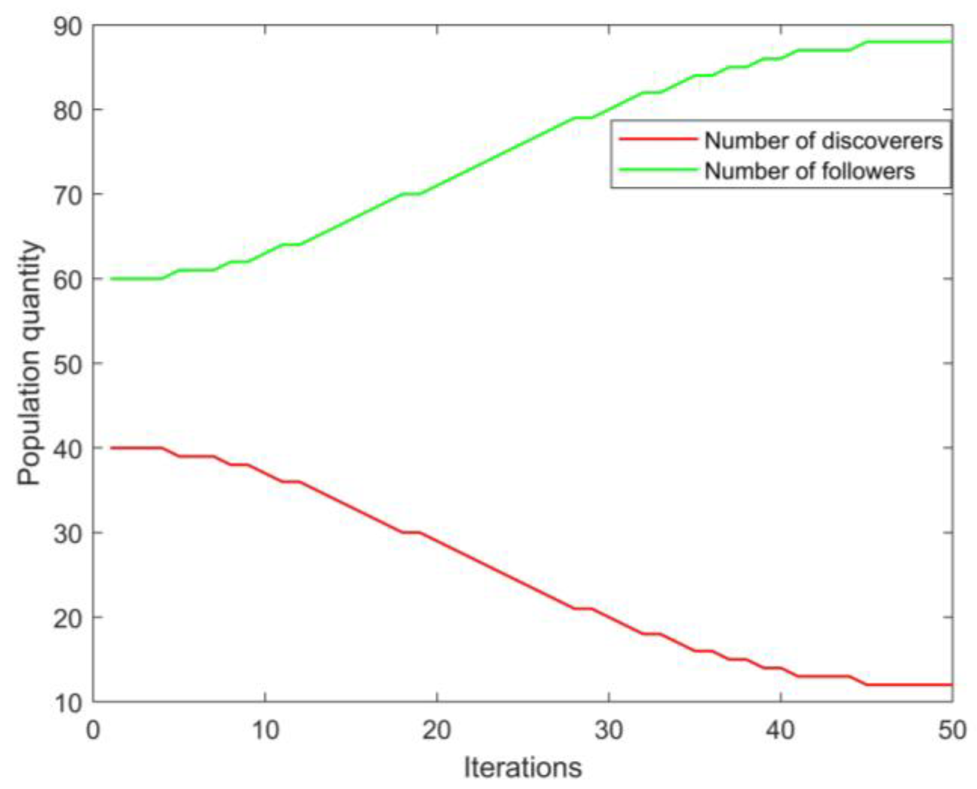
3.2. Discoverer–Follower Number Adaptive Adjustment Strategy

According to the principle of SSA, it is known that the number of discoverers and followers is fixed, and their identities will change according to the advantages and disadvantages of fitness in the iteration. The discoverers have a stronger global search ability, and the followers have a stronger local search ability due to the position adjustment formula. However, the number of discoverers is generally 10–20% of the population size, which will lead to a lack of ability to guide the global exploration of the population in the early stage of population iteration, and the lack of accurate local search ability in the later stage when the number of followers is insufficient. To this end, an adaptive adjustment strategy for the number of sparrows was proposed in this paper. The principle was as follows: as the number of iterations increased, the number of discoverers and followers showed a nonlinear decreasing and increasing trend, respectively, to increase the global optimization ability of the algorithm in the early stage and the local search ability in the later stage. The change range in the number of discoverers was set to be 40% to 10% of the population size. The specific formula is as follows:

$$\begin{array}{c}\gamma =\lambda \times \cos \left[\sin \left(\frac{t-1}{T}\times \frac{\pi }{2}\right)\right]\\ \mathrm{P}\mathrm{D}=\mathrm{r}\mathrm{o}\mathrm{u}\mathrm{n}\mathrm{d}\left(\gamma \times \mathrm{p}\mathrm{o}\mathrm{p}\right)\\ \mathrm{P}\mathrm{H}=\mathrm{p}\mathrm{o}\mathrm{p}-\mathrm{P}\mathrm{D}\end{array}$$

(4)

where $\gamma$ represents the adaptive adjustment coefficient, $\lambda$ is the proportionality coefficient, which takes the value of 0.4 due to the range of variation in the number of discoverers, $T$ is set to 50, PD is the number of discoverers, and PH is the number of followers. When the population size is 100, the change in the number of discoverers and followers is shown in Figure 2.

3.3. Adaptive t-Distribution Variation

As the number of iterations increases, the sparrow will gradually move towards the current optimal value, resulting in a denser distribution of positions. However, it is difficult to determine whether the position is globally optimal at this time; and if it is locally optimal, it may cause the algorithm to pause and thus cannot escape the local extreme value. Therefore, in order to increase the diversity of the population and improve the search ability of the algorithm, this paper introduced an adaptive t-distribution to mutate the position of the discoverer in the current iteration.

The adaptive t-distribution is a new form of statistical distribution proposed by the British mathematical statistician Gosset, also known as the student distribution, whose shape of the probability density curve is determined by the degree of freedom, and the probability density function is:

$$f\left(x\right)=\begin{array}{cc}\frac{\tau \left(\frac{n+1}{2}\right)}{\sqrt{2\pi }\times \tau \left(\frac{n}{2}\right)}\times {\left(1+\frac{x^2}{n}\right)}^{-\frac{n+1}{2}}& -\infty <x<+\infty \end{array}$$

(5)

where $\tau (x)$ is the gamma function, $n$ is the degree of freedom, when $n=1$, t-distribution is Cauchy distribution, when $n\to \infty$, it is Gaussian distribution.

Under different degrees of freedom, the t-distribution curve is shown in Figure 3. It can be seen from the figure that the Gaussian distribution and the Cauchy distribution are the two boundaries of the adaptive t-distribution. By analyzing the probability density curve, the probability of the Cauchy distribution obtaining a larger value is higher than that of the Gaussian distribution, so it has a strong global search ability. When $n=50$, the t-distribution curve almost coincides with the Gaussian distribution curve. In this paper, the current number of iterations was used as the degree of freedom. As the number of iterations increases, the curve shape gradually approaches the Gaussian distribution from the Cauchy distribution, so that the mutation result in the early stage of the iteration has a strong global search ability, and the later stage has a strong local search ability.

The specific process is as follows: introduce dynamic variation probability ${\beta }_c$ and random number $\alpha$. When $\alpha <{\beta }_c$, use the adaptive t-distribution to mutate all current discoverer positions, calculate the fitness before and after mutation, and select the individual with the best fitness as the new optimal individual. When $\alpha >{\beta }_c$, no mutation operation was performed. The main purpose of introducing $\alpha$ and $\beta$ was to reduce the probability of mutation in the later iterations of the algorithm, to avoid variation operations even after obtaining the global optimal value, and to avoid increasing the time and complexity of the algorithm.

The calculation formula of dynamic mutation probability, random number, and position after mutation is as follows:

$$\begin{array}{c}{\beta }_c=\cos \left(\frac{iter}{T}\times \frac{\pi }{2}\right)\\ \alpha =\mathrm{rand}()\\ x_{i,j}^{*}=x_{i,j}+x_{i,j}\times t\left(iter\right)\end{array}$$

(6)

where $iter$ is the number of current iterations, $x_{i,j}$ is the i-th individual in the j-th dimension, $x_{i,j}^{*}$ is the individual after the $x_{i,j}$ variation, and $t(iter)$ is the adaptive t-distribution with degree of freedom $iter$.

4. Results and Discussion

4.1. ISSA Performance Test

In this paper, 23 sets of commonly used benchmark test functions [33] were selected to test the performance of ISSA and compared with SSA.

Table 1. Benchmark Function.

Function	Range	D	Fmin
$F_1(x)={\displaystyle {\sum }_{i=1}^n{x}_i^2}$	[−100, 100]	30	0
$F_2\left(x\right)={\displaystyle {\sum }_{i=1}^n\left|x_i\right|+{\displaystyle \prod _{i=1}^n\left|x_i\right|}}$	[−10, 10]	30	0
$F_3\left(x\right)={\displaystyle {\sum }_{i=1}^n{\left({\displaystyle {\sum }_{j-1}^i{x}_j}\right)}^2}$	[−100, 100]	30	0
$F_4\left(x\right)={\max }_i\left\{\left|x_i\right|,1\le i\le n\right\}$	[−100, 100]	30	0
$F_5\left(x\right)={\displaystyle {\sum }_{i=1}^{n-1}\left[100\left(x_{i+1}-x_i{}^2\right)+{\left(x_i-1\right)}^2\right]}$	[−30, 30]	30	0
$F_6\left(x\right)={\displaystyle {\sum }_{i=1}^n{\left(\left[x_i+0.5\right]\right)}^2}$	[−100, 100]	30	0
$F_7\left(x\right)={\displaystyle {\sum }_{i=1}^{n}i{x}_i{}^4+\mathrm{random}\left[0,1\right)}$	[−1.28, 1.28]	30	0
$F_8\left(x\right)={\displaystyle {\sum }_{i=1}^n-x_i\sin \left(\sqrt{\left|x_i\right|}\right)}$	[−500, 500]	30	−418.98 × D
$F_9\left(x\right)={\displaystyle {\sum }_{i=1}^n\left[x_i^2-10\cos \left(2\pi x_i\right)+10\right]}$	[−5.12, 5.12]	30	0
$F_{10}\left(x\right)=-20\exp \left(-0.2\sqrt{\frac{1}{n}{\displaystyle {\sum }_{i=1}^n{x}_i^2}}\right)-\exp \left(\frac{1}{n}{\displaystyle {\sum }_{i=1}^n\cos \left(2\pi x_i\right)}\right)+20+e$	[−32, 32]	30	0
$F_{11}\left(x\right)=\frac{1}{4000}{\displaystyle {\sum }_{i=1}^n{x}_i^2-{\displaystyle \prod _{i=1}^n\cos \left(\frac{x_i}{\sqrt{i}}\right)+1}}$	[−600, 600]	30	0
$\begin{array}{l}{F}_{12}\left(x\right)=\frac{\pi }{n}\{10\sin \left(\pi y_1\right)+{\displaystyle {\sum }_{i=1}^{n-1}{\left(y_i-1\right)}^2\left[1+10{\sin }^2\left(\pi y_{i+1}\right)\right]}+{\left(y_n-1\right)}^2\}\\ y_i=1+\frac{x_i+1}{4};u\left(x_i,a,k,m\right)=\left\{\begin{array}{c}k{\left(x_i-a\right)}^m\\ 0\\ k{\left(-x_i-a\right)}^m\end{array}\right.\begin{array}{c}{x}_i>a\\ -a<x_i<a\\ x_i<-a\end{array}\end{array}$	[−50, 50]	30	0
$\begin{array}{l}{F}_{13}\left(x\right)=0.1\{{\sin }^2\left(3\pi x_1\right)+{\displaystyle {\sum }_{i=1}^n{\left(x_i-1\right)}^2}\times \left[1+xi{n}^2\left(3\pi x_i+1\right)\right]+{\left(x_n-1\right)}^2\left[1+{\sin }^2\left(2\pi x_n\right)\right]\}\\ +{\displaystyle {\sum }_{i=1}^{n}u\left(x_i,5,100,4\right)}\end{array}$	[−50, 50]	30	0
$F_{14}\left(x\right)={\left[\frac{1}{500}+{\displaystyle {\sum }_{j=1}^{25}\frac{1}{j+{\displaystyle {\sum }_{i=1}^2{\left(x_i-a_i{}_j\right)}^6}}}\right]}^{-1}$	[−65, 65]	2	1
$F_{15}(x)={{\displaystyle {\sum }_{i=1}^{11}\left[a_i-\frac{x_1\left(b_i^2+b_1{x}_2\right)}{b_i{}^2+b_1{x}_3+x_4}\right]}}^2$	[−5, 5]	4	0.0003
$F_{16}\left(x\right)=4x_1^2-2.1x_1^4+\frac{1}{3}{x}_1^6+x_1{x}_2-4x_2^2+4x_2^4$	[−5, 5]	2	−1.0316
$F_{17}\left(x\right)={\left(x_2-\frac{5.1}{4{\pi }^2}{x}_1^2+\frac{5}{\pi }{x}_1-6\right)}^2+10\left(1-\frac{1}{8\pi }\right)\cos x_1+10$	[−5, 5]	2	0.398
$\begin{array}{l}{F}_{18}\left(x\right)=[1+{\left(x_1+x_2+1\right)}^2]\times \left(19-14x_1+3x_1^2-14x_2+6x_1{x}_2+3x_2^2\right)\\ \times [30+{\left(2x_1-3x_2\right)}^2\times \left(18-32x_1+12x_1^2+48x_2-36x_1{x}_2+27x_2^2\right)]\end{array}$	[−2, 2]	2	3
$F_{19}\left(x\right)=-{\displaystyle {\sum }_{i=1}^4{c}_i\exp \left(-{\displaystyle {\sum }_{j=1}^3{a}_{ij}{\left(x_{ij}-p_{ij}\right)}^2}\right)}$	[1, 3]	3	−3.86
$F_{20}\left(x\right)=-{\displaystyle {\sum }_{i=1}^4{c}_i\exp \left(-{\displaystyle {\sum }_{j=1}^6{a}_{ij}{\left(x_{ij}-p_{ij}\right)}^2}\right)}$	[0, 1]	6	−3.32
$F_{21}\left(x\right)=-{{\displaystyle {\sum }_{i=1}^5\left[\left(X-a_i\right){\left(X-a_i\right)}^T+c_i\right]}}^{-1}$	[0, 10]	4	−10.1532
$F_{22}\left(x\right)=-{{\displaystyle {\sum }_{i=1}^7\left[\left(X-a_i\right){\left(X-a_i\right)}^T+c_i\right]}}^{-1}$	[0, 10]	4	−10.4028
$F_{23}\left(x\right)=-{{\displaystyle {\sum }_{i=1}^{10}\left[\left(X-a_i\right){\left(X-a_i\right)}^T+c_i\right]}}^{-1}$	[0, 10]	4	−10.5363

lists the expressions, search ranges, dimensions and optimal values of the benchmark functions, where F1–F7 are unimodal functions, F8–F13 are multimodal functions, and F14–F23 are fixed-dimensional multimodal functions. The range in the table indicates the search range of the independent variable x, D indicates the dimensionality of the benchmark functions, and $F_{\min }$ indicates the optimal value of the function result. The unimodal function contains an extreme point, which is mainly used to test the global search ability and convergence speed of the algorithm; the multimodal function contains multiple extreme points, which is mainly used to test the local search ability of the algorithm; and the fixed-dimensional multimodal function is used to test the ability of the function to avoid local optimum problems [33]. To ensure the reliability and fairness of the experiments, all experiments were carried out on a laptop computer (the specific model is Hasee Z7-KP7DC, Shenzhen, China) with Windows 10 operating system and a CPU of Intel Core i7-8750H. The simulation software was MATLAB2020B. The experimental parameters were set as follows: the population size $N$ was 30, and the maximum number of iterations T was 1000. The best value (best), worst value (worst), average value (aver), and standard deviation (std) of the results of 30 runs of ISSA and SSA on each test function were used to evaluate the performance of the algorithm, where the best data were marked in bold, and the final data were shown in

Table 2. Benchmark function test results (the optimal data is displayed in bold).

		Best	Aver	Worst	Std
F1	SSA	1.86557543252123 × 10−242	1.51061153412230 × 10−31	2.75307698567120 × 10−30	5.88942497435157 × 10−31
	ISSA	0	4.27081085628363 × 10−220	1.28124306546856 × 10−218	0
F2	SSA	3.592764117337923 × 10−69	1.05215088499046 × 10−20	2.43515575039904 × 10−19	4.53784333352281 × 10−20
	ISSA	1.84978498166486 × 10−251	4.29094165698757 × 10−111	1.28568003884339 × 10−109	2.34722079918870 × 10−110
F3	SSA	1.57252444000000 × 10−316	1.75380114435615 × 10−29	5.24283828182607 × 10−28	9.57092940402367 × 10−29
	ISSA	0	4.08090592234734 × 10−216	1.18669288637180 × 10−214	0
F4	SSA	0	2.68229508846477 × 10−15	7.48325233341391 × 10−14	1.36387615638502 × 10−14
	ISSA	0	4.23113317831045 × 10−110	1.26933880920409 × 10−108	2.31748492435314 × 10−109
F5	SSA	7.37154207400960 × 10−10	1.01500859821868 × 10−06	8.92127514819244 × 10−06	1.82490752625067 × 10−06
	ISSA	2.02843770289964 × 10−08	3.21506718912247 × 10−05	0.000306574454002731	6.12484232097627 × 10−05
F6	SSA	1.56911637210232 × 10−12	4.19577804214889 × 10−10	3.33187941051024 × 10−09	7.42866519675952 × 10−10
	ISSA	1.01094813931186 × 10−09	1.78671987291765 × 10−07	7.13605599408916 × 10−07	1.91302170819916 × 10−07
F7	SSA	1.80477227557695 × 10−05	0.000198096255476805	0.000528324129619586	0.000121590006922501
	ISSA	5.27992087356204 × 10−06	0.000142503068818720	0.000405066308104379	9.21025478001756 × 10−05
F8	SSA	−11,237.3936187566	−9657.18320228176	−4579.19580237451	2896.59237596103
	ISSA	−12,569.1802910539	−11,269.3676884736	−9123.99096788646	1684.18987077972
F9	SSA	0	0	0	0
	ISSA	0	0	0	0
F10	SSA	8.88178419700125 × 10−16	7.40148683083438 × 10−15	1.21680443498917 × 10−13	2.30635643744382 × 10−14
	ISSA	8.88178419700125 × 10−16	8.88178419700125 × 10−16	8.88178419700125 × 10−16	0
F11	SSA	0	0	0	0
	ISSA	0	0	0	0
F12	SSA	1.27509765131711 × 10−12	3.20233465455875 × 10−09	4.27856730875005 × 10−08	9.80134028046934 × 10−09
	ISSA	9.00023672308502 × 10−11	1.94549274675890 × 10−08	1.97480880547144 × 10−07	4.16506384216889 × 10−08
F13	SSA	1.84551272423733 × 10−11	2.58346876541052 × 10−08	2.88453177196628 × 10−07	6.67681501393322 × 10−08
	ISSA	1.36344744810396 × 10−11	5.68536045532780 × 10−07	4.12656208404738 × 10−06	9.85108667605740 × 10−07
F14	SSA	0.998003837794450	10.7790901579504	12.6705058111356	3.68791818335545
	ISSA	0.998003837874042	9.10878963650822	12.6705058111356	5.23300836072021
F15	SSA	0.000307492589579077	0.000314072147588383	0.000338641964046121	8.43080111283077 × 10−06
	ISSA	0.000307490742550469	0.000311706465277887	0.000334894582494230	6.28323981896366 × 10−06
F16	SSA	−1.03162845348988	−1.03162845348988	−1.03162845348988	5.23183651370722 × 10−16
	ISSA	−1.03162841956848	−1.03162845227174	−1.03162845348988	6.18203052512082 × 10−09
F17	SSA	0.397887357736325	0.397887357729958	0.397887357729738	1.20252259235403 × 10−12
	ISSA	0.397887359151452	0.397887357777177	0.397887357729738	2.59559338214047 × 10−10
F18	SSA	2.99999999999994	2.99999999999993	2.99999999999992	3.31916413768800 × 10−15
	ISSA	3.00000000000000	3.00000000000160	3.00000000003893	7.08653172659052 × 10−12
F19	SSA	−0.300478907194946	−0.300478907194947	−0.300478907194946	2.25840514163348 × 10−16
	ISSA	−1.49167852264867	−0.986643720836295	−0.491061108810976	0.268605209990880
F20	SSA	−3.32199517069621	−3.24277992836144	−3.13162152458857	0.0769381219422981
	ISSA	−3.32195416785194	−3.27710827822330	−3.19200891896637	0.0600220205695463
F21	SSA	−10.1531996788662	−9.98326627360475	−5.05519772893287	0.930763554085670
	ISSA	−10.1531996790582	−10.1530522023380	−10.1493123664807	0.000708596958649054
F22	SSA	−10.4029403823562	−9.87138850942744	−5.08767182506027	1.62183185350483
	ISSA	−10.4028967931467	−10.4029283303084	−10.4029405667897	4.63028789889682 × 10−05
F23	SSA	−10.5364098155995	−10.5364023952920	−10.5361871795855	4.06477576396309 × 10−05
	ISSA	−10.5363318802579	−10.5364043533081	−10.5364098118706	1.46076002558824 × 10−05

. The average results of 30 runs were selected to draw iteration curves; Figure 4 showed the iteration curves of the unimodal and multimodal test functions, and Figure 5 showed the iteration curves of the fixed-dimensional multimodal function.

4.1.1. Analysis of Test Results

Analyzing the data in Table 2, in the test of unimodal functions, ISSA successfully found the optimal value of the function in F1, F3 and F4, while SSA only found the optimal value in F4. The results of ISSA are better than those of SSA in the other three metrics of F1, F3 and F4, which means that ISSA has better global search ability and stability. Among the four functions that did not find optimal results, the performance indicators obtained by ISSA in F2 and F7 are much better than SSA, but the performance in F5 and F6 is weaker than SSA. Therefore, in the test of unimodal function, ISSA’s performance is slightly stronger than SSA, and its global search ability is stronger.

In the test of multimodal function, ISSA and SSA reach the optimal value of 0 for all four parameters in F9 and F11, and the performance index obtained by ISSA is much better than that of SSA in F8, but the performance is weaker than that of SSA in F12. In F10, the best obtained by the two is the same, but the remaining three parameters of ISSA are better than those of SSA, which proves that its performance is more stable. In F13, ISSA obtained a better best but the other three parameters are inferior to SSA, indicating that its local search ability is better but the stability is slightly worse. Therefore, ISSA performs slightly better than SSA in the test of multimodal function.

In the test of fixed-dimensional multimodal function, the four parameters obtained by ISSA in F15, F20, F21 and F22 are better than those of SSA. In F14, F16 and F17, the best and aver of ISSA are better, which means that ISSA has a better ability to find the optimum, but the result of std shows that its stability is slightly worse. In F18, ISSA successfully found the optimal value, but the other three parameters of SSA are better, which means ISSA successfully jumped out of the local extreme value at this time. In F19, the remaining three parameters of ISSA except std outperformed SSA, which proves ISSA’s search ability is stronger but its stability is slightly worse. In F23, only parameter aver of SSA is better than ISSA, and the other three parameters ISSA is better, which means that ISSA’s search ability and stability are stronger than SSA at this time. Therefore, in the test of fixed-dimensional multimodal function, the stability of ISSA is similar to that of SSA but the search ability is better than that of SSA, which means that the local optimum can be avoided with greater probability.

In summary, among the four evaluation metrics of the 23 benchmark test functions, at best, 16 results of ISSA are better than SSA, 4 results are equal to SSA, and 3 results are worse; on average, 15 results of ISSA are better than SSA, 2 results are equal to SSA, and 6 results are worse; at worst, 13 results of ISSA are better than SSA, 5 results are equal to SSA, and 5 results are worse; in std, 12 results of ISSA are better than SSA, 2 results are equal to SSA, and 9 results are worse. In summary, ISSA’s search ability and stability are better than SSA.

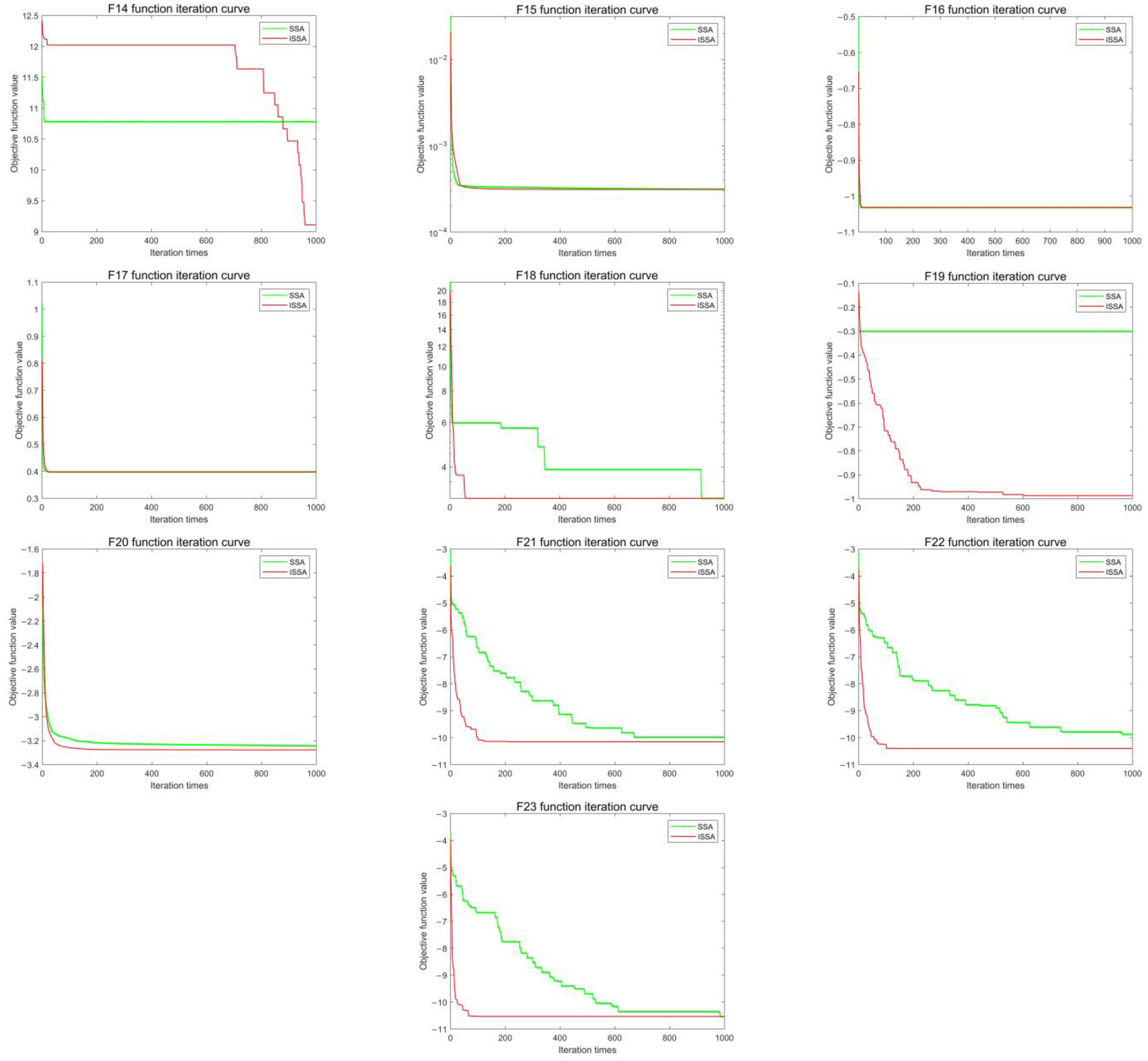
4.1.2. Iterative Curve Analysis

Observing the iterative curves of the unimodal test function in Figure 4, it can be seen that in F1–F4 and F7, the rate of decline and final values of ISSA curves are better than those of SSA. Only in F5 and F6 are the descent speed and final values of SSA curves better; therefore, the global search ability and convergence speed of ISSA are better than those of SSA in the test of unimodal function.

Observing the iterative curves of the multimodal test function in Figure 4, we can see that in F8, F10 and F11, the performance of ISSA is significantly better than that of SSA, with a faster decreasing speed of the curve and lower final value; in F9, the final values of both are the same and both reach the optimal value of 0, but the descent speed of the ISSA curve and the time to reach the optimal value are significantly better than SSA; only in F12 and F13 is the performance of SSA better than ISSA. Therefore, the local search ability and convergence speed of ISSA are better than those of SSA in the test of multimodal function.

Observing the iterative curves of the fixed-dimensional multimodal functions in Figure 5, it can be seen that in F18–F23, the rate of decline and the final values of ISSA curves are obviously better than those of SSA; in F15–F17, the two curves have a higher degree of overlap, especially in F16 and F17 where the two curves basically overlap; in the curve of F14, it can be observed that SSA has a better value of the preliminary objective function but falls into the local optimum, while ISSA can jump out of the local optimum and the final values are better than those of SSA, although the value of the preliminary objective function is worse.

In summary, among the 23 iterative curves of the benchmark test functions, 14 function curves of ISSA have a better descent speed and final values than SSA, 1 function curve has a fast decline speed but the same final value, 1 function curve has a slower decreased speed but the final value is better, 3 function curves basically overlap with SSA curves, and 4 function curves have a decreasing speed and final values inferior to SSA. In summary, the convergence speed and merit-seeking ability of ISSA are better than SSA.

By observing the iteration curves in Figure 4 and Figure 5, ISSA has better initial values than SSA in 18 functions, including F1–F5, F7–F12, F15–F18 and F21–F23, and only has worse initial positions in the remaining 5 functions. Therefore, it can be seen that the reverse good point set strategy produces better initial positions, and combined with the conclusions drawn from the summary of Section 4.1.1 and Section 4.1.2, it can be seen that the introduction of the discoverer–follower adjustment strategy and adaptive t-distribution successfully enhances the local search and global search ability of the algorithm, and the ability of the algorithm to jump out of the local optimum is enhanced to a certain extent.

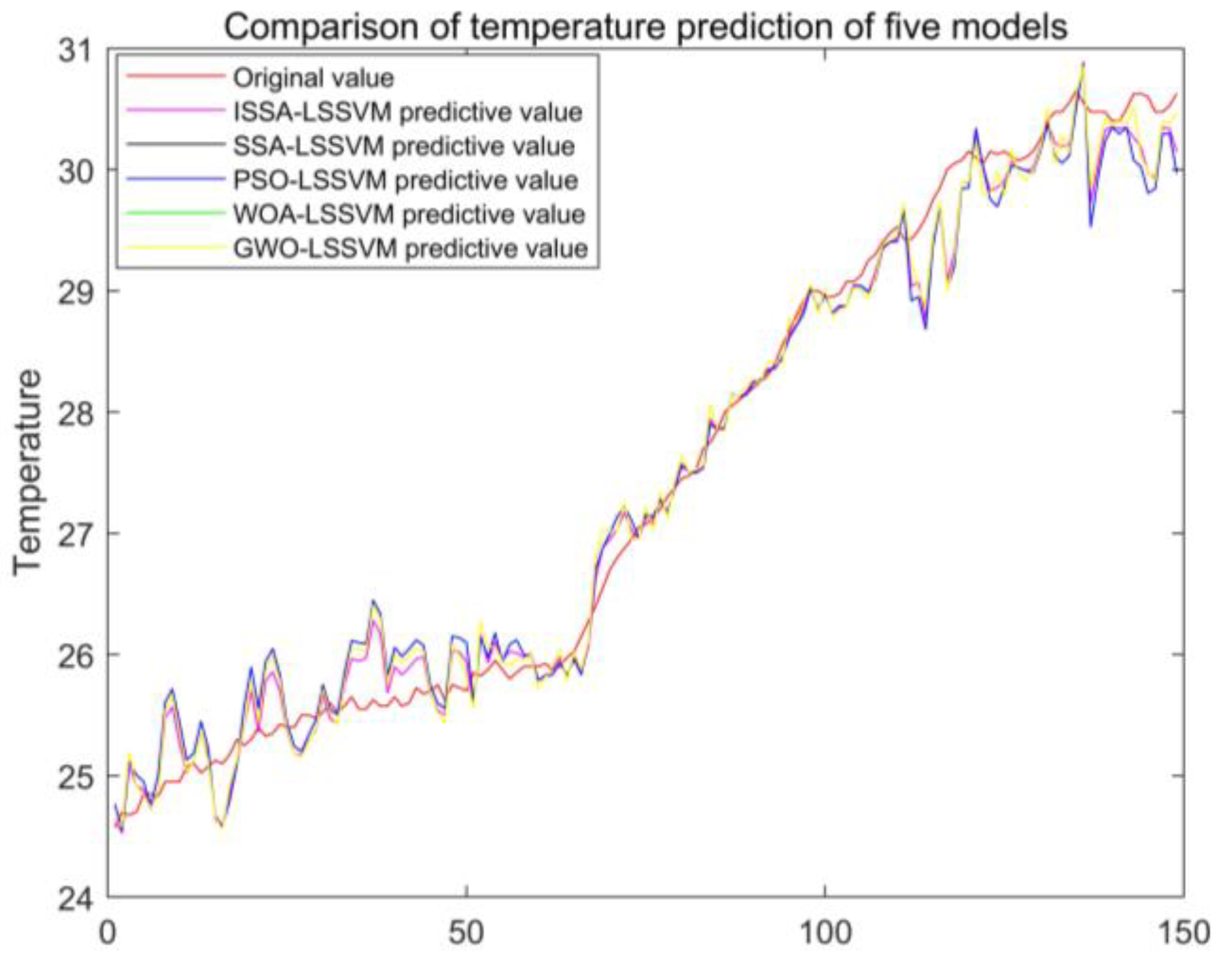
4.2. Comparison of Pig House Temperature Predictions

To further validate the performance of the proposed ISSA in practical applications, SSA, whale optimization algorithm (WOA), grey wolf optimization (GWO), and particle swarm optimization (PSO) were selected to optimize LSSVM for prediction comparison of the internal temperature of pig houses, the principle of the five intelligent optimization algorithms is the same. They all use their own position as the key parameter of LSSVM to predict the temperature in the house.

The internal temperature data of the pig house at the school teaching base in Qianguo County, Songyuan City, Jilin Province was used as the research object for predictive simulation analysis. The barn was divided into 4 areas by the middle cross aisle, temperature sensors were arranged in the center of each of the 4 areas with a height of 0.5 m from the ground, and the sampling time interval was 5 min. 1792 sets of data were detected. Considering that the temperature prediction process in this paper requires the data set to satisfy the time series, at the same time, in order to illustrate the generalization ability of the prediction model, the last block validation method in the out-of-sample evaluation method is used. Therefore, the first 1643 sets of data were selected as the model training data, and the last 149 sets of data were used as the test set for prediction accuracy testing. As mentioned in Section 2.1, using 20 min data to predict the next time data, that is, using 4 temperature data as input, the output prediction value corresponds to the fifth temperature.

The data was first preprocessed, including linear interpolation to fill in missing data, quadrature lookup to fill in outlier data, and data merging processing. To ensure the fairness of the prediction comparison, the algorithms all used the same parameter configuration: the population size $N$ pop was 100, the maximum number of iterations T was 50, and the parameters took the upper limit of 1000 and the lower limit of 0.01. The MSE, mean absolute error (MAE), and coefficient of determination (R²) were chosen to evaluate the prediction performance of the algorithms. The prediction curves of the five models are shown in Figure 6, and the values of the evaluation index are shown in

Table 3. Evaluation Index Values of Prediction Model.

	MAE	MSE	R2
ISSA-LSSVM	0.2105	0.0766	0.9818
SSA-LSSVM	0.2259	0.0895	0.9788
PSO-LSSVM	0.2590	0.1175	0.9721
GWO-LSSVM	0.2259	0.0895	0.9788
WOA-LSSVM	0.2259	0.0895	0.9788

.

From Figure 6, in the temperature prediction test, ISSA-LSSVM has the best prediction effect, and the other four have poor prediction effects. Among them, the temperature prediction values of the LSSVM models optimized by WOA and GWO are exactly the same so the green and yellow curves overlap completely, and only one yellow curve can be seen in the figure. By analyzing the data in Table 3, it can be found that compared with the other four prediction models, the MAE and MSE of ISSA-LSSVM are the smallest, and the R² value is the largest, which proves that the prediction effect is the best. The performance of SSA-LSSVM, GWO-LSSVM and WOA-LSSVM is close, and the prediction performance of PSO-LSSVM is the lowest.

5. Conclusions

In order to accurately predict the internal temperature changes of the pigsty, achieve stable control in advance, reduce energy consumption, and ensure the healthy and rapid growth of the pigs, this paper proposes an ISSA-optimized LSSVM temperature prediction model for the shortcomings of the SSA algorithm. The main contributions are as follows:

(1)

Taking into account the fact that SSA is prone to falling into a local optimum in the late iteration, the present study successfully enhanced SSA by employing three optimization methods: reverse good point set, adaptive parameter adjustment, and adaptive t-distribution variation.

(2)

To evaluate the performance of the ISSA proposed in this study, 23 benchmark test functions were chosen and tested in two aspects: convergence accuracy and convergence speed. When compared to SSA, the results showed that the ISSA proposed in this paper has higher convergence accuracy and speed, as well as stronger local and global search ability.

(3)

The prediction effect of the ISSA-LSSVM model was tested by comparing it to the LSSVM model optimized by four standard algorithms: SSA, PSO, GWO, and WOA. According to the results, the ISSA-LSSVM prediction model developed in this work achieved the best prediction effect and can provide accurate data support for the predictive control of the internal temperature of the pigsty.

References

1. Pexas, G.; Mackenzie, S.G.; Jeppsson, K.H.; Olsson, A.C.; Wallace, M.; Kyriazakis, I. Environmental and economic consequences of pig-cooling strategies implemented in a European pig-fattening unit. J. Clean. Prod. 2021, 290, 125784. [Google Scholar] [CrossRef]
2. Liu, F.; Zhao, W.; Le, H.H.; Cottrell, J.J.; Green, M.P.; Leury, B.J.; Dunshea, F.R.; Bell, A.W. Review: What have we learned about the effects of heat stress on the pig industry? Animal 2022, 16, 100349. [Google Scholar] [CrossRef] [PubMed]
3. Teixeira, A.D.R.; Veroneze, R.; Moreira, V.E.; Campos, L.D.; Januário, R.S.C.; Reis, F.C.P.H. Effects of heat stress on performance and thermoregulatory responses of Piau purebred growing pigs. J. Therm. Biol. 2021, 99, 103009. [Google Scholar] [CrossRef]
4. Howden, S.M.; Crimp, S.J.; Stokes, C.J. Climate change and Australian livestock systems: Impacts, research and policy issues. Anim. Prod. Sci. 2008, 48, 780–788. [Google Scholar] [CrossRef]
5. Carroll, J.A.; Burdick, N.C.; Chase, C.C.; Coleman, S.W.; Spiers, D.E. Influence of environmental temperature on the physiological, endocrine, and immune responses in livestock exposed to a provocative immune challenge. Domest. Anim. Endocrin 2012, 43, 146–153. [Google Scholar] [CrossRef]
6. Morteza, T.; Saman, A.M.; Abbas, R.; Majid, R.; Mostafa, R.J. Applied machine learning in greenhouse simulation; new application and analysis. IPA 2018, 5, 253–268. [Google Scholar]
7. Ayad, S.; Seyed, M.S. The effect of dynamic solar heat load on the greenhouse microclimate using CFD simulation. Renew. Energ. 2019, 138, 722–737. [Google Scholar]
8. Raphael, L.; Ido, S. Greenhouse temperature modeling: A comparison between sigmoid neural networks and hybrid models. Math. Comput. Simulat 2003, 65, 19–29. [Google Scholar]
9. Matej, G.; Robert, S.M.; Kevin, J.L. Forecasting indoor temperatures during heatwaves using time series models. Build. Environ. 2018, 143, 727–739. [Google Scholar]
10. Tian, W.; Zhang, X.; Lv, D.; Wang, L.; Liu, Q. Sliding mode control strategy of 3-UPS/S shipborne stable platform with LSTM neural network prediction. Ocean Eng. 2022, 265, 112497. [Google Scholar] [CrossRef]
11. Wen, J.; Chen, X.; Li, X.; Li, Y. SOH prediction of lithium battery based on IC curve feature and BP neural network. Energy 2022, 261, 125234. [Google Scholar] [CrossRef]
12. Dai, T.; Xiao, Y.; Liang, X.; Li, Q.; Li, T. ICS-SVM: A user retweet prediction method for hot topics based on improved SVM. Digit. Commun. Netw. 2022, 8, 186–193. [Google Scholar] [CrossRef]
13. Ye, Y.; Wang, L.; Wang, Y.; Qin, L. An EMD-LSTM-SVR model for the short-term roll and sway predictions of semi-submersible. Ocean. Eng. 2022, 256, 111460. [Google Scholar] [CrossRef]
14. Song, Y.; Xie, X.; Wang, Y.; Yang, S.; Ma, W.; Wang, P. Energy consumption prediction method based on LSSVM-PSO model for autonomous underwater gliders. Ocean. Eng. 2021, 230, 108982. [Google Scholar] [CrossRef]
15. Zhang, Y.; Li, R. Short term wind energy prediction model based on data decomposition and optimized LSSVM. Sustain. Energy Technol. 2022, 52, 102025. [Google Scholar] [CrossRef]
16. Narjes, N.; Sultan, N.Q.; Ely, S.; Alireza, B. Evolving LSSVM and ELM models to predict solubility of non-hydrocarbon gases in aqueous electrolyte systems. Measurement 2020, 164, 107999. [Google Scholar]
17. Chen, H.; Deng, T.; Du, T.; Chen, B.; Skibniewski, M.J.; Zhang, L. An RF and LSSVM–NSGA-II method for the multi-objective optimization of high-performance concrete durability. Cem. Concr. Comp. 2022, 129, 104446. [Google Scholar] [CrossRef]
18. Reza, G.G.; Reza, S.; Mohammad, T.; Mohsen, S.; Ghassem, Z. A novel PSO-LSSVM model for predicting liquid rate of two phase flow through wellhead chokes. J. Nat. Gas. Sci. Eng. 2015, 24, 228–237. [Google Scholar]
19. Huihui, Y.; Yingyi, C.; Shahbaz, G.H.; Daoliang, L. Prediction of the temperature in a Chinese solar greenhouse based on LSSVM optimized by improved PSO. Comput. Electron. Agr. 2016, 122, 94–102. [Google Scholar]
20. Liu, Y.; Cao, Y.; Wang, L.; Chen, Z.S.; Qin, Y. Prediction of the durability of high-performance concrete using an integrated RF-LSSVM model. Constr. Build. Mater. 2022, 356, 129232. [Google Scholar] [CrossRef]
21. Pan, X.; Xing, Z.; Tian, C.; Wang, H.; Liu, H. A method based on GA-LSSVM for COP prediction and load regulation in the water chiller system. Energ. Build. 2021, 230, 110604. [Google Scholar] [CrossRef]
22. Sadra, R.; Fariborz, R.; Hossein, S. Prediction of oil-water relative permeability in sandstone and carbonate reservoir rocks using the CSA-LSSVM algorithm. J. Petrol. Sci. Eng. 2019, 173, 170–186. [Google Scholar]
23. Jiankai, X.; Bo, S. A novel swarm intelligence optimization approach: Sparrow search algorithm. J. Petrol. Sci. Eng. 2020, 8, 22–34. [Google Scholar]
24. Wu, H.; Zhang, A.; Han, Y.; Nan, J.; Li, K. Fast stochastic configuration network based on an improved sparrow search algorithm for fire flame recognition. Knowl.-Based Syst. 2022, 245, 108626. [Google Scholar] [CrossRef]
25. Zhang, Z.; Han, Y. Discrete sparrow search algorithm for symmetric traveling salesman problem. Appl. Soft Comput. 2022, 118, 108469. [Google Scholar] [CrossRef]
26. Xiong, J.; Liang, W.; Liang, X.; Yao, J. Intelligent quantification of natural gas pipeline defects using improved sparrow search algorithm and deep extreme learning machine. Chem. Eng. Res. Des. 2022, 183, 567–579. [Google Scholar] [CrossRef]
27. Li, J.; Lei, Y.; Yang, S. Mid-long term load forecasting model based on support vector machine optimized by improved sparrow search algorithm. Energy Rep. 2022, 8, 491–497. [Google Scholar] [CrossRef]
28. Kathiroli, P.; Selvadurai, K. Energy efficient cluster head selection using improved Sparrow Search Algorithm in Wireless Sensor Networks. J. King Saud. Univ.-Com. 2021, 34, 8564–8575. [Google Scholar] [CrossRef]
29. Azaza, M.; Echaieb, K.; Tadeo, F.; Fabrizio, E.; Iqbal, A.; Mami, A. Fuzzy Decoupling Control of Greenhouse Climate. Arab. J. Sci. Eng. 2015, 40, 2805–2812. [Google Scholar] [CrossRef]
30. Dan, X.; Shangfeng, D.; Gerard, V.W. Double closed-loop optimal control of greenhouse cultivation. Control Eng. Pract. 2019, 85, 90–99. [Google Scholar]
31. He, G.; Lu, X. Good point set and double attractors based-QPSO and application in portfolio with transaction fee and financing cost. Expert. Syst. Appl. 2022, 209, 118339. [Google Scholar] [CrossRef]
32. Ren, L.; Liu, T.; Zhao, Q.; Yang, J.; Cao, Y. Method for Measurement Uncertainty Evaluation of Cylindricity Error Based on Good Point Set. Procedia CIRP 2018, 75, 373–378. [Google Scholar]
33. Ma, J.; Hao, Z.; Sun, W. Enhancing sparrow search algorithm via multi-strategies for continuous optimization problems. Inform. Process. Manag. 2022, 59, 102854. [Google Scholar] [CrossRef]
Figure 1. Two-dimensional initialization data distribution comparison.
Agriculture 13 01710 g001
Figure 2. Changes in the number of finders and followers.
Agriculture 13 01710 g002
Figure 3. T distribution curve.
Agriculture 13 01710 g003
Figure 4. Test of convergence characteristics of two algorithms (1).
Agriculture 13 01710 g004
Figure 5. Test of convergence characteristics of two algorithms (2).
Agriculture 13 01710 g005
Figure 6. Predicted contrast curve.
Agriculture 13 01710 g006