Article

Assessing Spatial Variation and Driving Factors of Available Phosphorus in a Hilly Area (Gaozhou, South China) Using Modeling Approaches and Digital Soil Mapping

College of Natural Resources and Environment, South China Agricultural University, Guangzhou 510642, China
*
Author to whom correspondence should be addressed.
Agriculture 2023, 13(8), 1541; https://doi.org/10.3390/agriculture13081541
Submission received: 10 June 2023 / Revised: 29 July 2023 / Accepted: 30 July 2023 / Published: 2 August 2023
(This article belongs to the Special Issue Soil Degradation and Remediation)

Abstract

:
Soil fertility plays a crucial role in crop growth, so it is important to study the spatial distribution and variation of soil fertility for agricultural management and decision-making. However, traditional methods for assessing soil fertility are time-consuming and economically burdensome. Moreover, it is hard to capture the spatial variation of soil properties across continuous geographic space using the conventional methods. As key techniques of digital soil mapping (DSM), spatial interpolation techniques have been widely applied in soil surveys and analysis in recent years, since they can predict soil properties at unknown points in continuous space based on limited sample points. However, further research is needed on spatial interpolation models for DSM in regions with variable climates and complex terrains, which are characterized by strong spatial variation in both environmental variables and soil fertility. In this study, taking a typical hilly area in a subtropical monsoon climate, i.e., Gaozhou, Guangdong Province, China, as an example, the performances of four popular spatial interpolation models (Random Forest (RF), Ordinary Kriging, Inverse Distance Weighting, and Radial Basis Function) for digital soil mapping on available phosphorus (AP) are compared. Based on RF, the spatial variation and its driving factors of the AP of Gaozhou are then analyzed. Furthermore, by selecting three typical truncation lines from different directions, the correlations between environmental variables and AP in different spatial positions are demonstrated. The root mean square error (RMSE) results of the above four models are 32.01, 32.08, 32.74, and 33.08, respectively, which indicate that the RF has a higher interpolation accuracy. Based on the mapping results of RF, the minimum, maximum, and mean values of AP in the study area are 38.90, 95.24, and 64.96 mg/kg, respectively. The high-value areas of AP are mainly distributed in forested and orchard areas, while the low-value areas are primarily found in urban and cultivated areas in the eastern and western regions. Vegetation and topography are identified as the key factors shaping the spatial variations of AP in the study area. Furthermore, the spatial heterogeneity of the influence strength of altitude and EVI is revealed, providing a new direction for further research on DSM in the future, i.e., spatial interpolation models considering the spatial heterogeneity of the influence of environmental variables.

1. Introduction

In recent years, the contradiction between limited land resources and population growth has become increasingly prominent, and the efficient utilization of land productivity has become an urgent issue [1]. Soil fertility, as the foundation of land agricultural productivity, plays a crucial role, and obtaining high-precision spatial and attribute information about soil fertility is of great significance for land resource management and precision agriculture [2]. Traditional survey methods mainly involve collecting soil samples within a study area, recording their spatial coordinates and determining soil nutrients in the laboratory, followed by expert analysis of the results. However, these approaches require the collection and testing of a large number of samples, which consumes a significant amount of time and economic resources [3]. Moreover, they fail to visually demonstrate the spatial distribution characteristics and spatial variation patterns of soil properties in the study area [4]. Digital soil mapping (DSM) technology can use limited sample points to predict soil properties at unknown points, then obtain a soil fertility distribution map of the entire study area, and allow for an analysis of the driving factors that shape the spatial distribution characteristics and variation pattern of soil fertility, which has become a research hotspot [5,6,7,8].
Currently, DSM primarily relies on spatial interpolation techniques [4], which can be categorized into three main types based on the interpolation model: deterministic spatial interpolation methods [9,10,11,12], geostatistics-based uncertainty interpolation methods [7,13,14], and machine learning methods [15,16,17]. Deterministic spatial interpolation methods mainly include inverse distance weighting (IDW) [9], polynomial interpolation [11,12], and radial basis function (RBF) [10]. IDW establishes the relationship between the predicted point and the sampled points within the defined neighborhood based on the distance decay, where the influence of sampled points on the prediction increases as they approach the predicted point [9]. Polynomial interpolation captures the trend of the prediction data based on global [11] or local [12] sampled points by constructing polynomial functions. When constructing polynomial functions for local sampled points, the study area is first divided into multiple sub-regions, and multiple planes are then fitted to each sub-region, respectively, which can capture the characteristics of local variation within the study area. RBF utilizes the attribute values of each known sampled point within the study area to construct an RBF model and fits an observation surface for the entire study region [10]. In [18], with a forested catchment in Southern Arizona, USA, as an example, a least-squares linear regression model was constructed to learn the correlations between soil properties and environmental variables. An IDW model was then used to interpolate the regression residual. The above combination can capture the correlation between soil properties and the environment, and map the uncertainty of the mapping results. The methods mentioned above have the advantage of quickly constructing prediction models for large spatial areas. However, except for local polynomial interpolation, they struggle to capture the spatial variation characteristics of the data. Moreover, the local polynomial interpolation model requires a manual delineation of sub-region locations and a determination of sub-region sizes, and in order to capture the spatial variation characteristics of the data, it ignores the global correlation between each sub-region.
The second category is the geostatistics-based methods, which is represented by the Kriging series algorithms, such as Ordinary Kriging (OK) [13] and Universal Kriging [14]. These methods establish a variogram based on known sampled points to express the spatial autocorrelation of the spatial objects and predict the attributes of unknown points. In [19], an artificial neural network Ordinary Kriging (ANN-Kriging) algorithm is proposed for soil organic matter (SOM) mapping, which divides the mapping process into two stages. In the first stage, the neural network describing the relationship between SOM and the environmental landscape structure is trained, and the SOM is estimated by a well-trained ANN. The residual of the ANN is then estimated by Kriging in the second stage. Finally, the mapping result of SOM is produced by combining the results of the above two stages. However, Kriging methods require the prediction target to satisfy the assumption of second-order stationarity, which assumes that the variance of attribute values between any two points with the same distance and direction in space is equal. This assumption is clearly not applicable to soil fertility interpolation, which exhibits strong spatial non-stationarity. Moreover, the Original Kriging methods only consider the spatial autocorrelation of the data, overlooking the issue of spatial heterogeneity. To incorporate spatial heterogeneity into Kriging, some researchers have proposed Stratified Kriging (SK) [7], which divides the study area into multiple homogeneous sub-regions and constructs variograms for different sub-regions independently. However, this method faces the same problem as local polynomial interpolation methods, which is how the study area is effectively stratified.
The last category is the machine learning (ML)-based interpolation methods, such as Random Forest (RF) [15,20] and Support Vector Machine (SVM) [16], which have been extensively studied by researchers in recent years due to their strong ability to capture features of data. Studies have shown that ML-based spatial interpolation methods, particularly RF, can effectively capture both the spatial autocorrelation and heterogeneity of the data, and rank the importance of environmental factors with respect to the predicted values [21]. In addition, environmental variables, as important factors driving soil genesis and development, can greatly improve the prediction ability of the model after selecting appropriate environmental variables as features to be added into the model [22]. The environmental variables used in the current DSM model mainly include five major soil-forming factors, i.e., soil-forming parent material, topography, biology, climate, and time [4]. For example, the vegetation factor (e.g., the Normalized Difference Vegetation Index (NDVI), the Ratio Vegetation Index (RVI), the Difference Vegetation Index, and the Soil-Adjusted Vegetation Index (SAVI) derived from remote sensing images) and the topographic variables derived from the digital elevation model (DEM) (e.g., plan curvature and profile curvature) were involved in an RF model to predict soil organic matter content [23]. In [24], the OK, Co-Kriging, RF, and ANN were used to predict the soil fertility at parcel scale in China. The results showed that the RF has the highest accuracy at parcel scale among the four models. In [25], the RF model was used to map the soil classes in Northern Iran utilizing legacy soil maps as a covariate, which improves the accuracy of the model. However, the spatial variations and driving factors of soil available phosphorus (AP) in the coastal hilly areas of Southern China have seldom been studied using RF. Furthermore, current RF-based spatial interpolation models based on environmental variables assign equal weights to the environmental variables for the entire study area after training, with little consideration given to whether the influence strength of environmental variables varies across different spatial locations. The geographically weighted regression (GWR) methods [26] consider the varying influence strength of environmental variables across different spatial locations. However, in most GWR models, it only attenuates the influence strength based on distance. Incorporating anisotropy into GWR is still difficult. In addition, the GWR model is susceptible to the multicollinearity of environmental variables, which greatly reduces the prediction accuracy. In contrast, RF models are not sensitive to multicollinearity and have received much attention.
Motivated by the above considerations, taking Gaozhou as the study area, this paper first uses four popular spatial interpolation models (Random Forest, Ordinary Kriging, inverse distance weighting, and radius basis function) for the DSM of AP in Gaozhou. Subsequently, the spatial variations and driving factors of AP are analyzed based on the RF model. Additionally, an analysis is conducted to determine the correlation between AP and environmental variables, and the heterogeneity of the influence strength of the environmental variables is revealed. The major contributions of this study are summarized as follows:
  • The performance of four popular models (RF, IDW, RBF, and OK) for DSM of AP are shown and compared in a typical hilly area in a subtropical monsoon climate, i.e., Gaozhou.
  • The spatial distribution and variation characteristics of AP in the study area are analyzed.
  • The importance of driving factors that influence the spatial distribution and variation of AP are ranked and analyzed based on RF.
  • The correlation between AP and the influence of environmental variables at different spatial locations and directions are investigated, which reveals the spatial heterogeneity of the influence strength of the environmental factors.

2. Materials and Methods

2.1. Materials

2.1.1. Study Area

The study area is located in Gaozhou, Guangdong, China, with an administrative area of approximately 3276 km2. As shown as Figure 1, Gaozhou is geographically situated between 110°36′46″ E and 110°22′45″ E and between 21°42′34″ N and 22°18′49″ N. Based on the report of the local government (refer to http://www.gaozhou.gov.cn/gzgk/gzjs/content/post_896018.html (accessed on 13 March 2023)), it falls within a subtropical monsoon climate zone, characterized by abundant sunlight and rainfall. The average annual temperature of air is 24.5 °C. The average annual precipitation is 1628.3 mm, and the annual sunshine hours are 1769 h. The topography of Gaozhou is complex, comprising hills, basins, and plains. Overall, the terrain is higher in the northeast and lower in the southwest, with the mountainous areas accounting for about one-tenth of the total area. The highest point is located in the northeastern mountainous region, while the lowest point is in the southwestern riverbed. The above complex environment has brought great challenges to the digital soil mapping of soil fertility.
Gaozhou makes a significant contribution to the agricultural output of Guangdong, with a value reaching approximately 16.587 billion yuan (2.313 billion dollars) in 2021, comprising 24.5% of the regional gross domestic product. The cultivated area for grain crops exceeds 60,000 ha, which accounts for about 82% of the 36,238 ha under the double-cropping system. Its cash crops are mainly oil tea, oil tree, rubber, wampee, guava, pomelo, etc. Crops are biannual or tri-ripe, and this can generate substantial economic benefits. Thus, investigating the spatial variation and driving factors of soil fertility in this area is of great scientific and practical significance.

2.1.2. Data

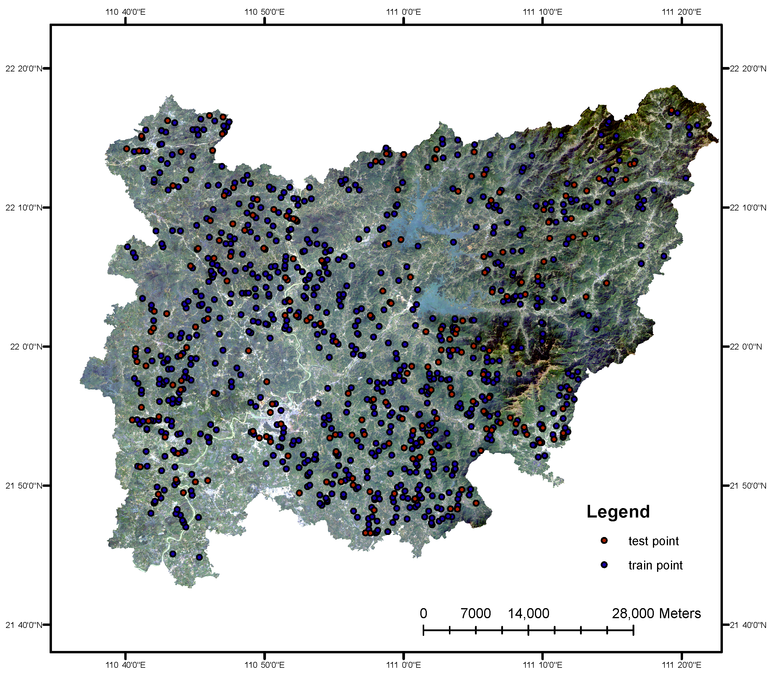
This study is based on a total of 986 soil samples collected from the soil layer of 0–20 cm of the study area using a stratified random sampling approach [27], and their AP content was determined by the Olsen method [28]. Considering the influence of different land use types on the spatial variation of soil fertility, the sampling was stratified according to the land use classification and randomly sampled in different plots. These samples are divided into training and testing sets in an 8:2 ratio, with 789 and 197 samples, respectively. The distribution of the training and testing sample sets is shown in Figure 2.
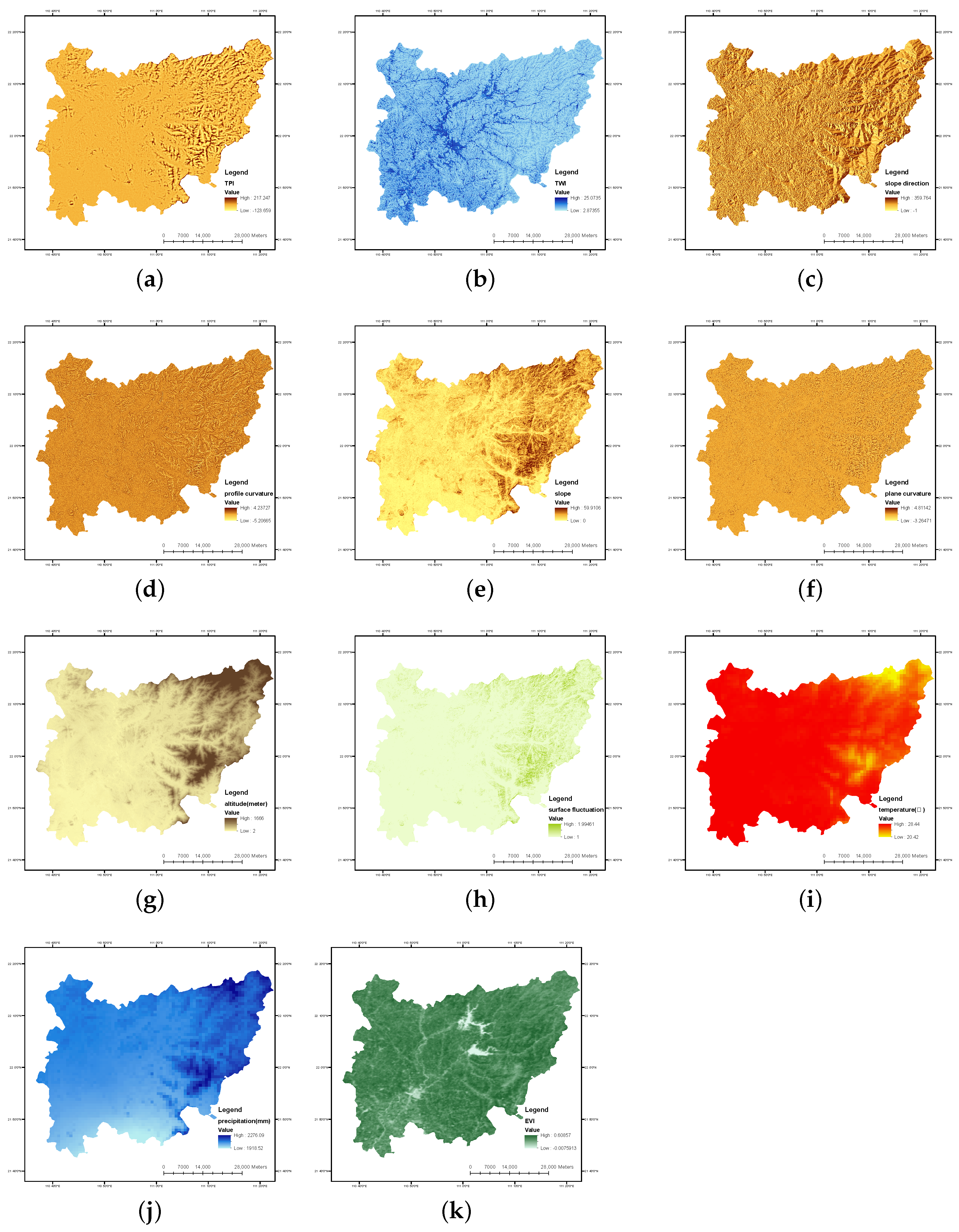
Subsequently, considering that the terrain, hydrological, climate, and biological conditions may affect the forming, transformation, and transportation process of phosphorus [29,30,31], 11 relative environmental variables were selected as auxiliary data for the model. These variables include the topographic position index (TPI), topographic wetness index (TWI), aspect, profile curvature, slope, plane curvature, altitude, surface fluctuation, average annual temperature, average annual precipitation, and enhanced vegetation index (EVI). Among these, the TPI, TWI, aspect, profile curvature, slope, plane curvature, altitude, and surface fluctuation can reflect the terrain and hydrological conditions from different dimensions, as they impact the ability of water flows to erode and transport AP. For example, AP is more susceptible to erosion and translocation in ridge areas due to the flowing water, while in valley areas, AP is more likely to be abundant [29]. In terms of climate conditions, the average annual temperature and average annual precipitation are included. Since the vegetation conditions can reflect the biomass [32], the EVI is considered as one of the covariates. It should be noted that parent material is also an important factor influencing AP content, but the high cost of investigation and the difficulty of obtaining data on parent material in the study area meant that it had to be regrettably excluded as a covariate.
The EVI was derived from Landsat 8 remote sensing images, while the average annual temperature and precipitation were interpolated from meteorological station data in Gaozhou. The remaining data were obtained by processing the digital elevation model (DEM) data of the study area from https://srtm.csi.cgiar.org/srtmdata (accessed on 13 March 2023)). All environmental variables are organized in raster format with a pixel size of 30 m, and their spatial distribution is shown in Figure 3.

2.2. Methods

The RF model, validation method, and truncation lines analysis method will be explained in this section, while the details of OK, IDW, and RBF can be found, respectively, in [9,10,33].

2.2.1. Random Forest for Spatial Interpolation

RF is an ensemble learning method that combines multiple classification or regression trees [34]. In the context of interpolation problems, the RF algorithm first repeatedly selects a certain number of samples from the dataset through bootstrapping, and these samples are used as training samples for each tree. During the training process of each tree, the node splits are performed by randomly selecting a subset of features from all available features for comparison. Through multiple iterations, multiple decision trees are constructed, with each decision tree trained on randomly selected training samples and features. Finally, the predictions from the multiple decision trees are aggregated using weighted summation to obtain the final prediction results. Typically, the average of predictions from multiple trees is used as the final prediction value, which is shown as Figure 4.
For spatial interpolation, there are many ways to incorporate spatial information into the RF model, such as including spatial coordinates [35] or distance maps [36] as covariates. Reference [21] reported a Random Forest Spatial Interpolation (RFSI) algorithm that considers spatial context information, i.e., neighboring observations and their distances to the target points, as covariates, which exhibits high performance in many spatial interpolation applications. However, when the sample points are unevenly distributed, modeling with neighboring sample points may reduce the interpolation accuracy in areas with sparse sample points and drastic environmental changes, such as areas of drastic terrain changes. Adding neighboring samples as covariates to the model may also weaken the importance of the remaining essential environmental variables in the model, further deepening the adverse effects on the sparsely distributed areas of sample points. Therefore, the RF model used in this study only considers environmental variables as covariates. Since the distribution of the environmental variables that shape the distribution of the target variables is characterized by spatial autocorrelation, the model still has the ability to implicitly learn the spatial structure of target variables from the environmental variables [21], which has been observed in maps predicted by RF in numerous studies [15,20,21].
The spatial interpolation model based on RF used in this study can be expressed as follows:
v = P ( x s , x p , c )
where  v  represents the predicted values for all target points,  P ( )  is the RF model,  x s  and  x p  represent all known sampled points and all target points data, respectively, and  c  is the input environmental variable data corresponding to the sampled points and target points.
Furthermore, the RF model can identify the environmental variables that play a crucial role in the model’s prediction results through importance ranking. Each decision tree constructed mentioned above uses the Gini importance measure of each environmental variable to assess its ability to partition samples. Subsequently, for each environmental variable, the average importance value across all decision trees is calculated to determine its overall importance. Finally, the importance of all environmental variables is ranked.

2.2.2. Validation Methods

For validating the performance of the spatial interpolation models, the sample data were divided into a training set and a testing set with 789 and 197 samples, respectively. The training set was used for model training, while the testing set was used for model validation. The root mean square error (RMSE, Equation (2)) was used to measure the accuracy of the interpolation results, which can indicate the overall error by comparing the predicted values and the observed values of the testing samples set.
R M S E = i = 1 n ( x i x i ) 2 n
where n is the number of points in the testing set.  x i  and xi are the predicted value and observed value of the ith point, respectively.

2.2.3. The Truncation Line Analysis Method

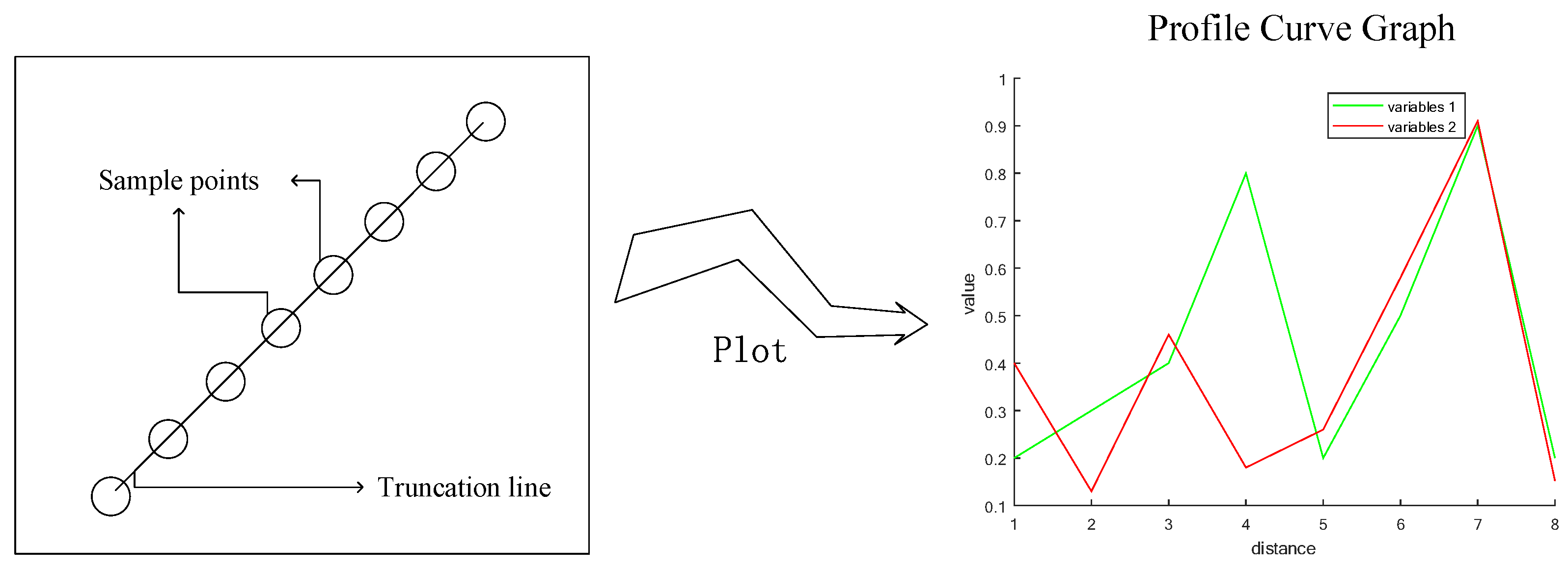
As shown in Figure 5, in the truncation line analysis method, the truncation line is delineated in the continuous space, the variable values on the line are extracted by uniform sampling, and the curve graph of the values of multiple variables on the line is drawn. By plotting the values of multiple variables on the same line, the correlation of different variables at different positions on the line can be visually observed, and this method has been widely used in many studies to analyze the relationship between multiple variables [37,38]. In this study, the correlation, spatial differentiation, and anisotropy of variables were analyzed by selecting truncation lines from different directions.

2.2.4. Statistical Analysis

The variance inflation factor (VIF) [39] and the Pearson correlation coefficient (PCC) [40] were used as statistical analysis methods in this study. VIF is an index to measure the collinearity between variables, which can be formulated as [39]
V I F ( x , y ) = 1 1 r 2 ( x , y )
where x and y are two random variables, and  r 2  is the coefficient of determination obtained by fitting a model for x and y.
PCC is the quotient of the covariance and standard deviation between two variables, which can be used to measure the correlation between two variables, which is defined as [40]
ρ ( x , y ) = E ( x y ) σ x σ y
where  ρ ( x , y )  is the PCC between x and y, and  σ x 2 = E ( x 2 )  and  σ y 2 = E ( y 2 ) .

3. Results

3.1. Results of the Digital Soil Mapping Based on Four Different Spatial Interpolation Models

Based on the sampling points and environmental variable data described in Section 2.1, the RF model was employed to predict the AP across the entire study area. To provide a more comprehensive analysis and highlight the differences and advantages of the RF model, three popular spatial interpolation models, including OK, IDW, and RBF, were also utilized to predict AP in the study area under the same condition. The results obtained from these three models were then compared with RF.

3.1.1. Parameters Setting

For the RF model, there are two important parameters, namely “n-tree” and “m-try”, which control the number of decision trees in RF and the number of features randomly selected from all features for each decision tree, respectively. The values of these parameters impact the generalization ability and computational speed of the model. As per recommendations in a previous study [34], the “n-tree” and “m-try” were set to 500 and the square root of the total number of features, i.e., 3, respectively. As for OK, IDW, and RBF models, their parameters were set as follows:
  • For OK, the nugget, partial sill, lag size, and the number of lags were set to 958.4114, 277.2129, 1150.591, and 12, respectively. The Gaussian Model was chosen as the semivariogram model.
  • For IDW, the power was set to 1.
  • For RBF, the kernel function and parameter were set to Completely Regularized Spline and 0.0846, respectively.
  • The mapping unit for all models, i.e., pixel size, was set to 30 m.

3.1.2. Mapping Results Analysis of Different Models

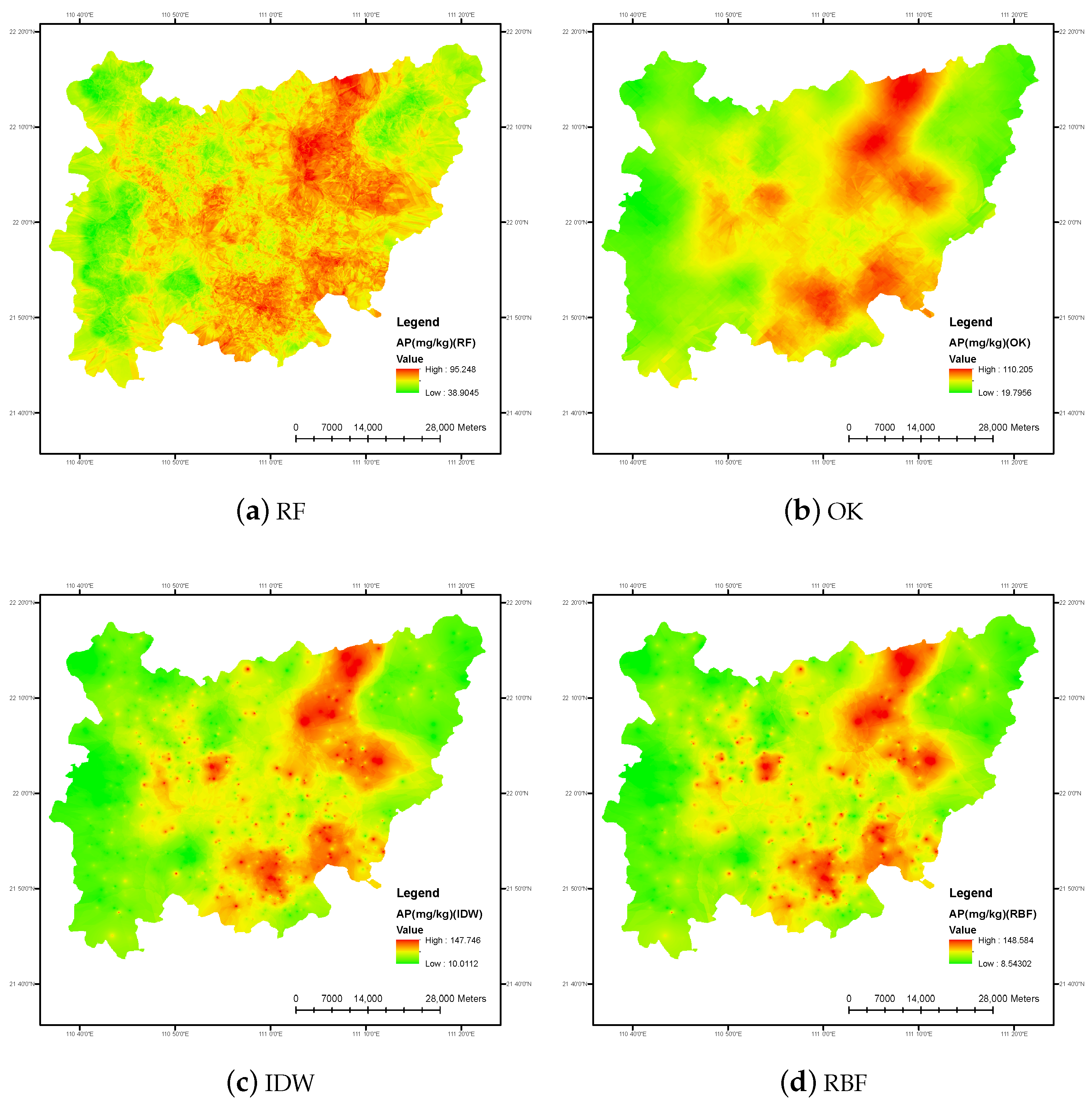
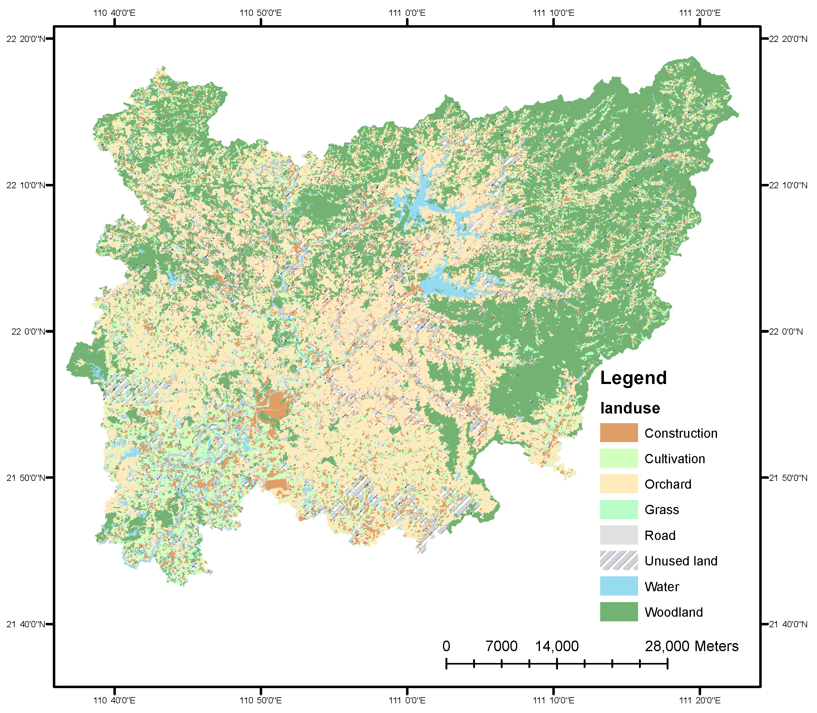
Under the above setting, the four models were trained using the training dataset, and the mapping results of AP were obtained by the four models as shown in Figure 6. In Figure 1 and Figure 6, it can be observed that the distribution of AP in the study area exhibits a certain spatial pattern. Specifically, the high-value and low-value areas of AP were concentrated in the study area. From Figure 7, the high-value areas are mainly distributed in the orchard and forested regions between 111° E and 111°10′ E in the central part of the study area, while the low-value areas are mainly distributed in the urban and cultivated regions, as well as the orchard area near the urban region and in the eastern and western parts of the study area. The above distribution results show that the content of AP is correlated with the type of vegetation and human activities on the surface. Based on the mapping results of RF, the minimum, maximum, and mean values of AP in the study area are 38.90, 95.24, and 64.96 mg/kg, respectively. Among the four conducted spatial interpolation models, the OK, IDW, and RBF models yield relatively smooth results, but the local distribution and variation characteristics of AP are not easily captured. On the contrary, the RF model produces a more detailed prediction result and thus shows a stronger ability to capture the spatial heterogeneity of the data, making it more suitable for soil fertility interpolation in complex geographical environments. Furthermore, the RMSE was used to measure the mapping accuracy of the models, and the accuracy of the four models was validated using the testing dataset. The RMSE results are shown in Table 1, and these results indicate that the RF model exhibits smaller prediction errors compared to other models, while the RBF has the largest error among the four methods.

3.2. Spatial Variation Analysis of Available Phosphorus over the Study Area

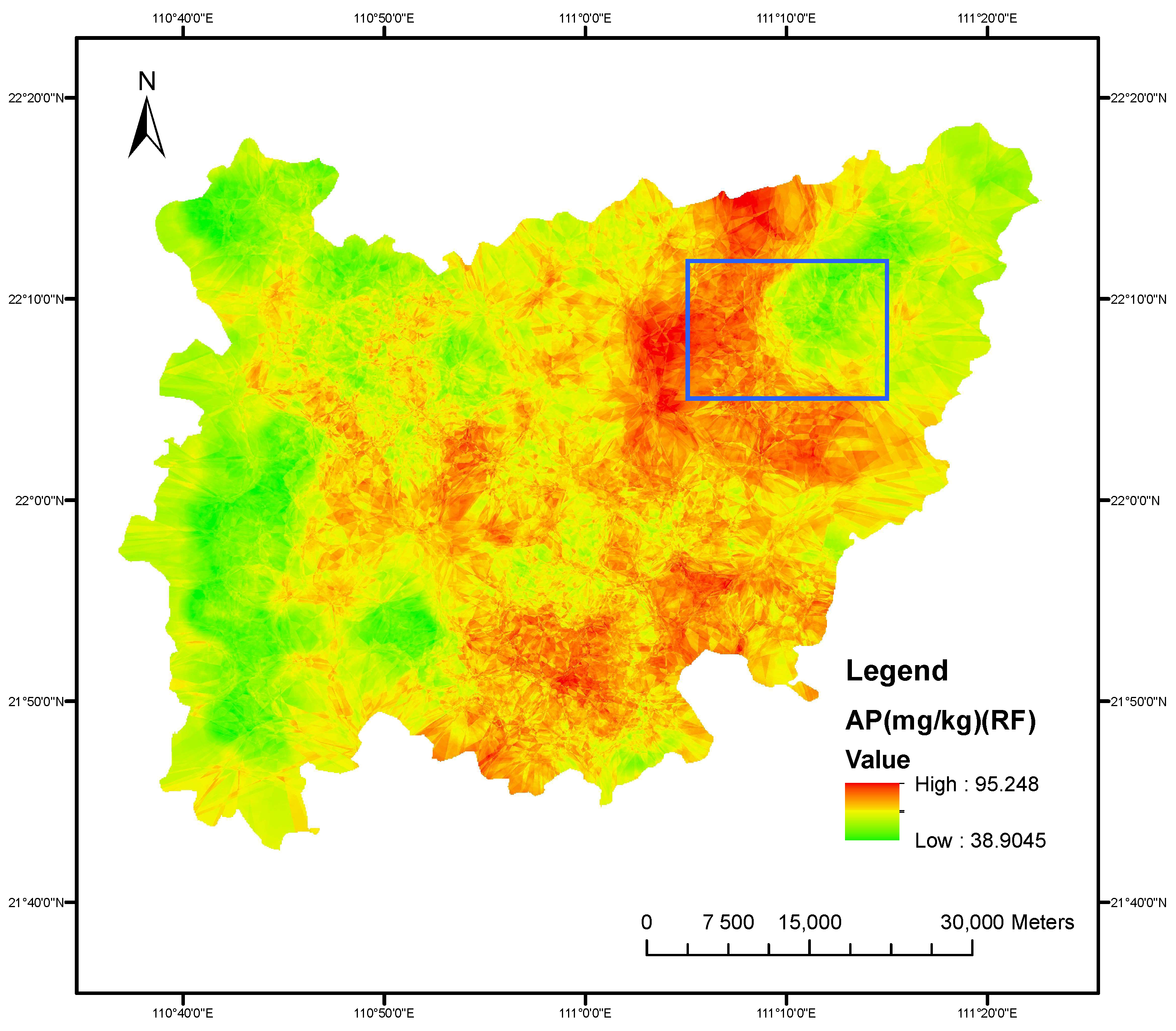
From the mapping results (Figure 6), it can be observed that the AP of the soil in Gaozhou exhibits significant spatial heterogeneity, which means that it does not have the same distribution characteristics in all sub-regions of the study area, indicating non-stationarity and anisotropy in its spatial variations. For example, in the region defined by the blue rectangle in Figure 8, a drastic change from a high to a low value of AP can be observed in the northeast direction, while a relatively stable variation is exhibited in the southwest direction. To explore the role of the geographical environment in shaping the spatial variation of AP in Gaozhou, the RF method was first used to rank the importance of influencing factors and identify the key factors affecting the AP content. Afterwards, by plotting the values of the environmental variables and AP on typical truncation lines, the correlation of the key factors and AP was further visually demonstrated.
Under the settings described in Section 3.1.1, the RF method was used to rank the importance of the environmental variables used in the RF model in this study. The results are shown in Table 2. The importance of the 11 environmental factors is ranked in descending order as follows: EVI, altitude, average annual precipitation, average annual temperature, slope, TPI, TWI, surface fluctuation, plane curvature, profile curvature, and aspect. The results indicate that biological, topographic, and climatic environmental variables are key factors influencing the AP in the study area, with elevation playing a primary role among the topographic variables.
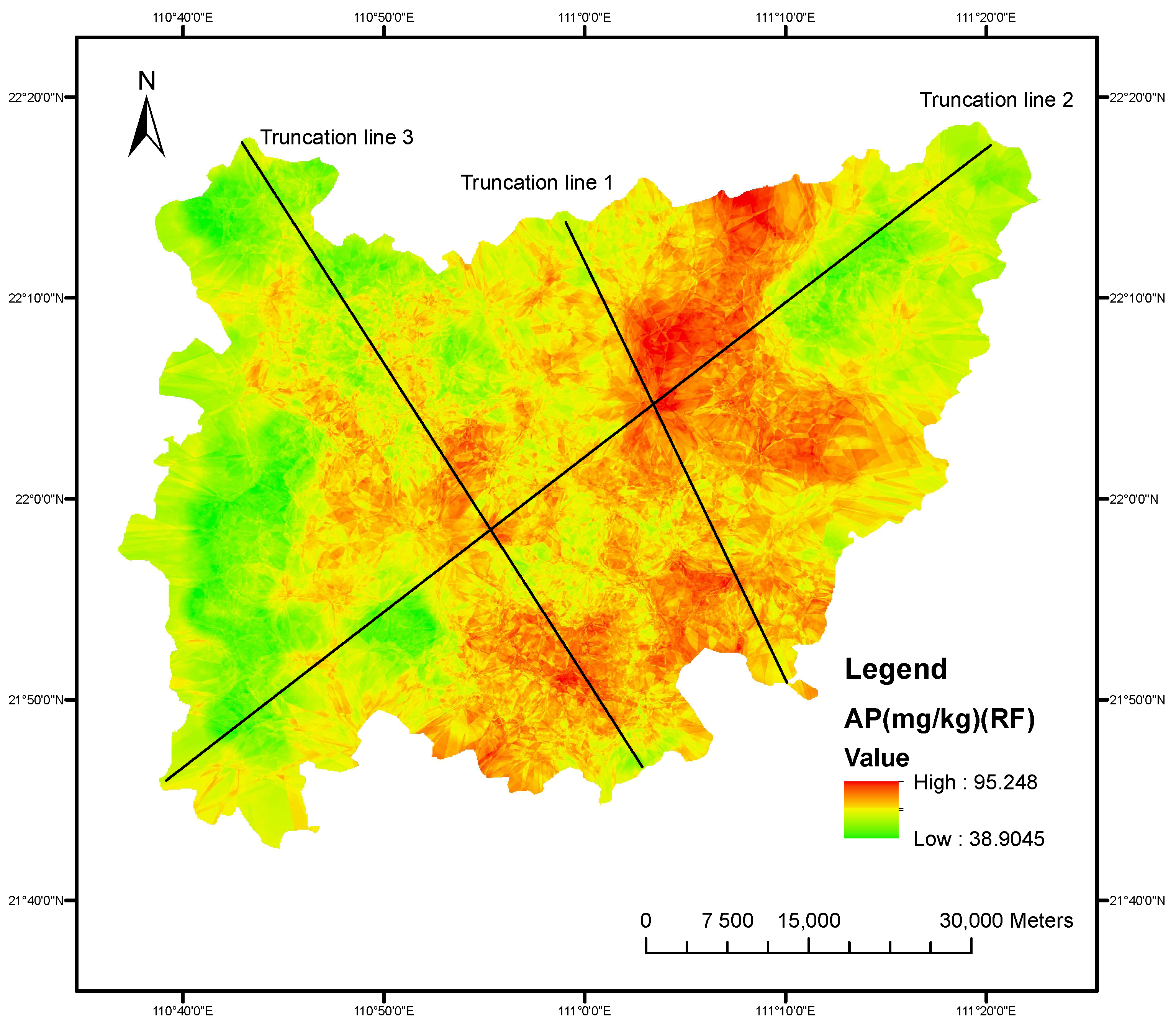
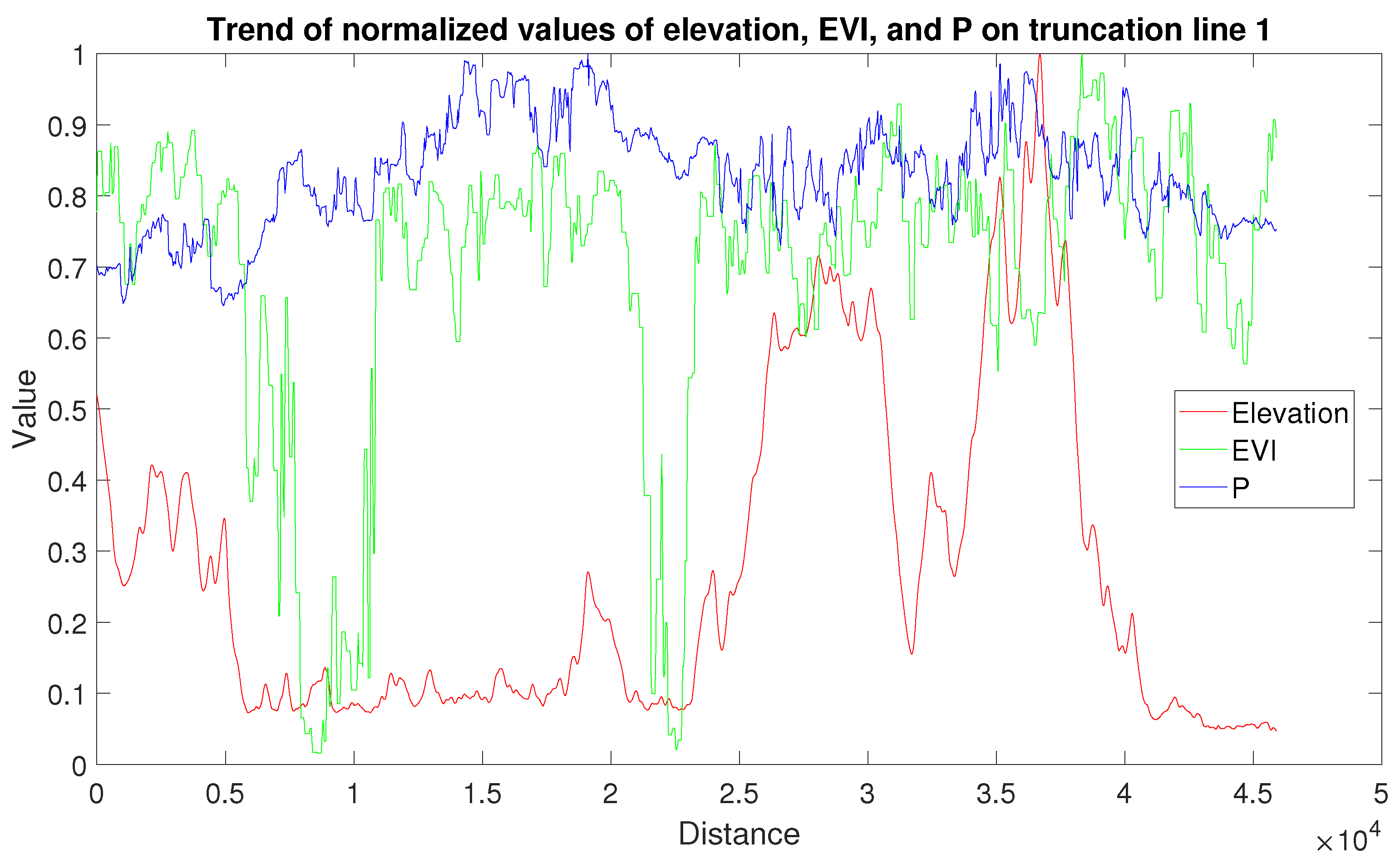
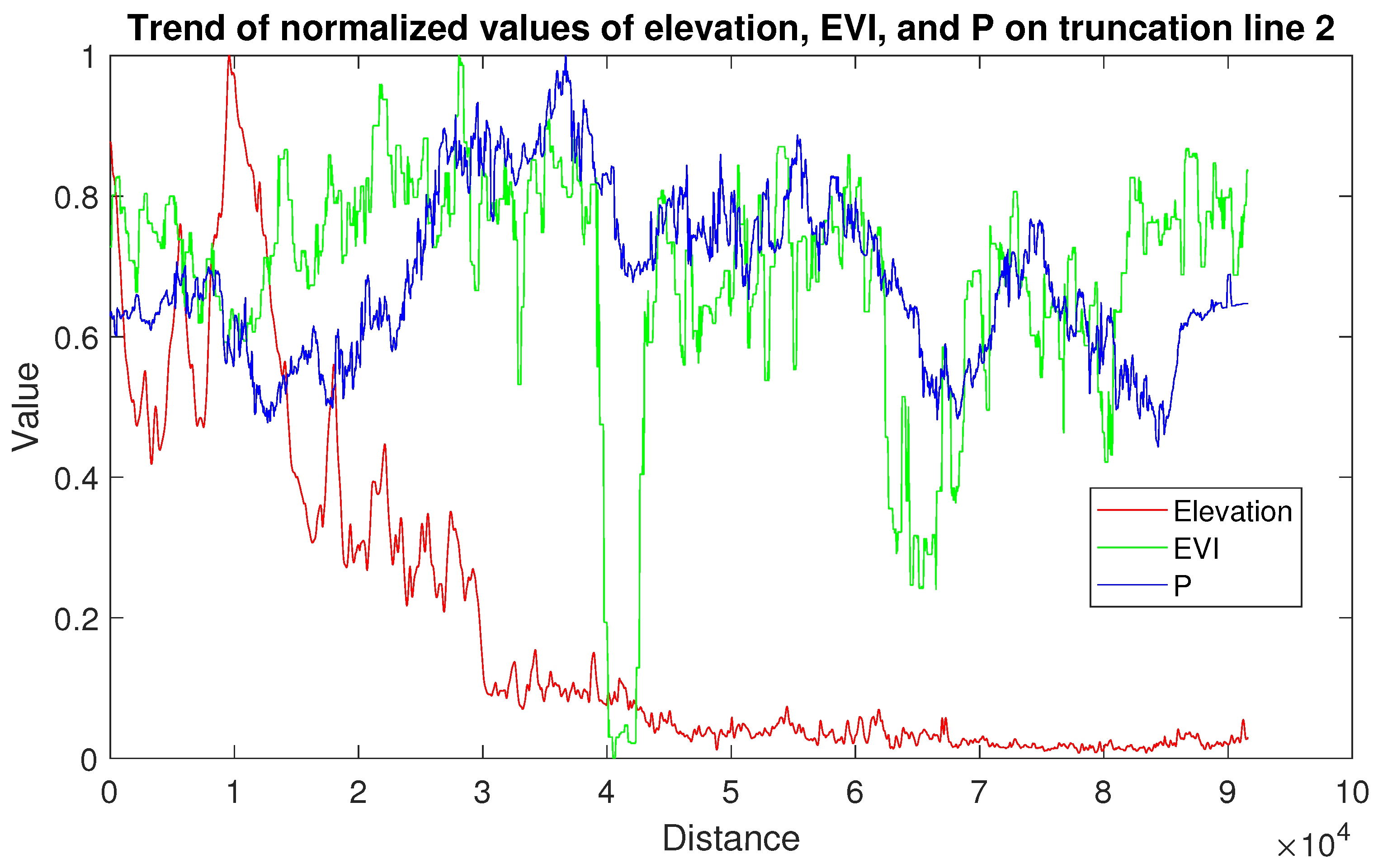
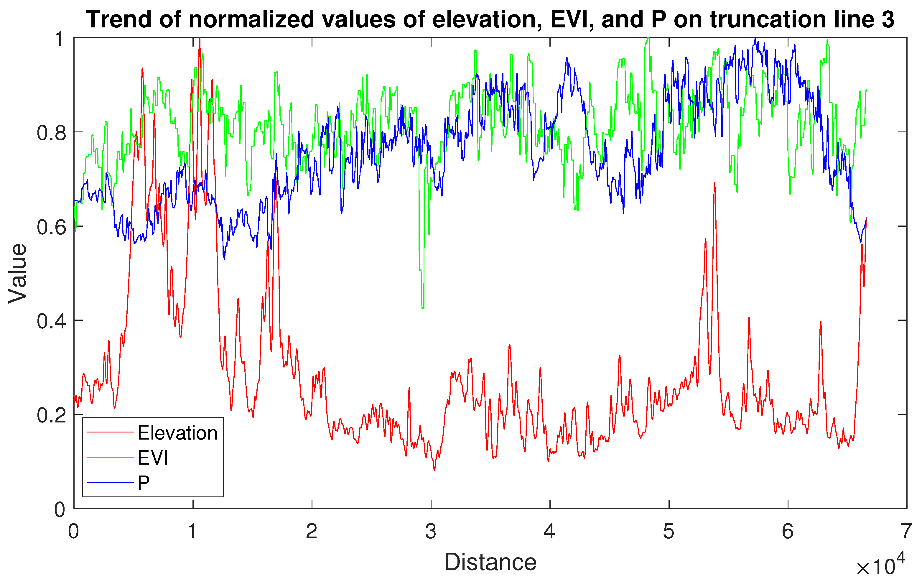
Although the importance ranking of environmental factors by RF indicates their respective importance, it does not capture the relationship between the environmental factors and AP so as to further reveal the actual impact of these factors on AP. Therefore, by selecting truncation lines in typical areas within the study area, a comparison was made between the variation trends of AP and environmental variables along these lines. This analysis aims to explore the spatial relationship between environmental factors and AP. The selection of the truncation lines was based on the criterion that there should be a significant change in AP and the key environmental factors along the lines, which aims to reveal underlying relationships through significant variation characteristics. Three truncation lines were selected, as shown in Figure 9. To ensure the representative of the results, the top two ranked factors, EVI and altitude, were chosen as the key environmental factors for analysis. Since the RF model provides more precise predictions, its results were used as a reference for AP in the study area. The analysis results are presented in Figure 10, Figure 11 and Figure 12.
In Figure 10, it can be observed that a positive correlation exists between AP and altitude along Truncation Line 1 within the distance of 0–0.5, while the negative and positive correlations are shown at distances of 1.25–1.75 and 3–3.75, respectively. In the remaining part of Truncation Line 1, there appears to be no significant correlation discernible from the visual analysis of the graph. Furthermore, the relationship between EVI and AP demonstrates a positive correlation within the distance of 0–0.4, followed by a negative correlation within the distance of 0.4–1. These findings collectively highlight the presence of distinct correlations between AP, EVI, and altitude along the same truncation line concurrently. In Figure 11 and Figure 12, it can also be observed that the correlation between EVI, altitude, and AP varies in different spatial positions along the same truncation line. The analysis of these three truncation lines, which pass through different typical areas from different directions, indicates that the influence of environmental factors on AP varies in different spatial positions and directions. This suggests the presence of spatial heterogeneity, i.e., spatial non-stationarity and anisotropy, in the influence strength of environmental variables, which are seldom considered in the spatial interpolation model conventionally used for digital soil mapping.

4. Discussion

4.1. Diagnosis for Collinearity of Key Driving Factors

To exclude the possibility of collinearity between the two key factors (i.e., altitude and EVI) causing the results observed in Figure 10, Figure 11 and Figure 12, the VIF and PCC mentioned in Section 2.2.4 were used. A  V I F 5  or  V I F 10  indicates strong collinearity among the variables [39], and while PCC is close to 0, it indicates a weak correlation between variables [41]. The values of VIF and PCC between altitude and EVI are 1.01052 and 0.04535, respectively, which shows that the two variables have weak collinearity and a low correlation.

4.2. The Performance Comparison between the Four Models

In Figure 6, it can be observed that, from a global perspective, the RF produces more fine-grained results, while the OK, IDW, and RBF methods yield smoother results, but only reflect the overall trends. In [42], the conclusion that the RF model can achieve finer spatial resolution was also confirmed in the prediction of soil properties in the semi-arid zone of South India. From a local perspective, on the one hand, RF, by incorporating environmental variables as covariates into the model and not solely relying on observation points, can make predictions even in areas with missing data points. For example, in the unsampled region at the western boundary of the study area, OK, IDW, and RBF methods only predicted values based on the distance-decayed values of neighboring sample points, resulting in an overall representation of low values (shown in green in Figure 6). In contrast, the mapping results of the RF model for the western region do not entirely exhibit low values; there are areas near the boundary that show higher values compared to the eastern part (shown in yellow in Figure 6), which may better satisfy the needs of seamless map integration at the boundaries. In [43], the authors also believe that the Kriging method may not be the best solution under the condition of sparse samples, which was also reported in [44]. On the other hand, the IDW and RBF methods generate numerous scattered high-value points that do not align well with natural features, leading to a lower quality of mapping. In summary, RF and their derived methods are recognized as superior performing mapping methods for a growing number of applications [20,21,36,45,46,47].
However, when comparing the results of RF and OK, the different trends observed in the mapping results of RF for the western region suggest that the mapping results based on RF may deviate from the distribution trend of known observation points. Based on the analysis results in Section 3.2, it can be speculated that this deviation might be attributed to spatial heterogeneity in the influence of the environmental variables. The RF assumes that the effect of covariates are consistent globally, which might lead to such deviations. For example, in flat terrain areas, vegetation may play a dominant role in affecting the AP content, while in steep terrain areas, the topography may primarily influence the AP content due to intensified erosion caused by the terrain [48]. In [49], a case study in the Loess Plateau of China provides insight into the spatially dependent correlations between soil properties and environmental factors from a regional perspective, which demonstrates that there are different factors controlling the spatial variation of the soil properties on a short-range scale and a long-range scale. Besides, as [50] reports, the scale heterogeneity may be enhanced by the interaction of nature or anthropogenic sources of variability. Thus, involving the spatial heterogeneity in the influence of the environmental variables into the model may increase the mapping accuracy, which can also provide more information about how the environment affects the AP content at different positions.

5. Conclusions

In this study, taking a typical hilly region, i.e., Gaozhou, as an example, an RF model for the digital soil mapping of AP was established and compared with three other popular spatial interpolation models: OK, IDW, and RBF. The results demonstrated that the RF model outperforms the other three interpolation algorithms in terms of interpolation accuracy and expression capability under the same conditions, since it can indirectly learn the spatial structure of the environmental variables. Based on the mapping results of the RF model, the spatial variation characteristics of AP in the study area were analyzed. The results revealed that high- and low-value areas of AP are relatively concentrated. Furthermore, using the RF importance ranking algorithm, the environmental factors shaping the spatial variation pattern of AP were ranked, and the altitude and EVI were identified as the key driving factors.
Moreover, based on the mapping results of the RF model, three truncation lines passing through typical areas where significant changes of key environmental variables and AP occur within the study area were selected to analyze the correlation between AP and environmental variables. The results revealed that, in addition to the spatial heterogeneity of environmental variables and AP, there is spatial heterogeneity in the influence strength of environmental variables on AP. This implies the presence of spatial non-stationarity and anisotropy in the influence strength of environmental variables, providing directions for further research on high-precision spatial interpolation and digital soil mapping methods considering the spatial heterogeneity of the influence strength of environmental variables.

Author Contributions

Conceptualization: W.Z. and J.X.; methodology: W.Z.; software: L.C.; validation: R.X., X.H. and W.M.; formal analysis: W.Z.; investigation: W.Z.; resources: J.X.; writing—original draft: W.Z.; writing—review & editing: W.Z.; supervision: J.X.; project administration: J.X.; funding acquisition: J.X. All authors have read and agreed to the published version of the manuscript.

Funding

This research received no external funding.

Institutional Review Board Statement

Not applicable.

Informed Consent Statement

Not applicable.

Data Availability Statement

Not applicable.

Acknowledgments

The authors are grateful to the editors and reviewers for their valuable comments and suggestions.

Conflicts of Interest

The authors declare no conflict of interest.

References

  1. Jin, M.; Wang, L.; Ge, F.; Xie, B. Understanding the Dynamic Mechanism of Urban Land Use and Population Distribution Evolution from a Microscopic Perspective. ISPRS Int. J. Geo-Inf. 2022, 11, 536. [Google Scholar] [CrossRef]
  2. Xu, T.; Yi, S.; Zhou, Y.; Li, Q.; Liu, Y. Temporal and Spatial Changes and Driving Forces of Soil Properties in Subtropical Mountainous Areas from 2017 to 2020: A Case Study of Baokang County, Hubei Province, China. Land 2022, 11, 1735. [Google Scholar] [CrossRef]
  3. Grunwald, S.; Thompson, J.; Boettinger, J. Digital soil mapping and modeling at continental scales: Finding solutions for global issues. Soil Sci. Soc. Am. J. 2011, 75, 1201–1213. [Google Scholar] [CrossRef] [Green Version]
  4. Zhang, G.L.; Feng, L.; Song, X.D. Recent progress and future prospect of digital soil mapping: A review. J. Integr. Agric. 2017, 16, 2871–2885. [Google Scholar] [CrossRef]
  5. Zhang, L.; Zhu, A.X.; Liu, J.; Ma, T.; Yang, L.; Zhou, C. An adaptive uncertainty-guided sampling method for geospatial prediction and its application in digital soil mapping. Int. J. Geogr. Inf. Sci. 2023, 37, 476–498. [Google Scholar] [CrossRef]
  6. Chen, S.; Arrouays, D.; Mulder, V.L.; Poggio, L.; Minasny, B.; Roudier, P.; Libohova, Z.; Lagacherie, P.; Shi, Z.; Hannam, J.; et al. Digital mapping of GlobalSoilMap soil properties at a broad scale: A review. Geoderma 2022, 409, 115567. [Google Scholar] [CrossRef]
  7. Liu, Y.; Chen, Y.; Wu, Z.; Wang, B.; Wang, S. Geographical detector-based stratified regression kriging strategy for mapping soil organic carbon with high spatial heterogeneity. Catena 2021, 196, 104953. [Google Scholar] [CrossRef]
  8. Minasny, B.; Berglund, Ö.; Connolly, J.; Hedley, C.; de Vries, F.; Gimona, A.; Kempen, B.; Kidd, D.; Lilja, H.; Malone, B.; et al. Digital mapping of peatlands—A critical review. Earth-Sci. Rev. 2019, 196, 102870. [Google Scholar] [CrossRef]
  9. Yasrebi, J.; Saffari, M.; Fathi, H.; Karimian, N.; Moazallahi, M.; Gazni, R. Evaluation and comparison of ordinary kriging and inverse distance weighting methods for prediction of spatial variability of some soil chemical parameters. Res. J. Biol. Sci. 2009, 4, 93–102. [Google Scholar]
  10. Bhunia, G.S.; Shit, P.K.; Maiti, R. Spatial variability of soil organic carbon under different land use using radial basis function (RBF). Model. Earth Syst. Environ. 2016, 2, 17. [Google Scholar] [CrossRef]
  11. Apaydin, H.; Sonmez, F.K.; Yildirim, Y.E. Spatial interpolation techniques for climate data in the GAP region in Turkey. Clim. Res. 2004, 28, 31–40. [Google Scholar] [CrossRef] [Green Version]
  12. Hani, A.; Abari, S.A.H. Determination of Cd, Zn, K, pH, TNV, organic material and electrical conductivity (EC) distribution in agricultural soils using geostatistics and GIS (case study: South-Western of Natanz-Iran). Int. J. Agric. Biosyst. Eng. 2011, 5, 852–855. [Google Scholar]
  13. Gia Pham, T.; Kappas, M.; Van Huynh, C.; Hoang Khanh Nguyen, L. Application of ordinary kriging and regression kriging method for soil properties mapping in hilly region of Central Vietnam. ISPRS Int. J. Geo-Inf. 2019, 8, 147. [Google Scholar] [CrossRef] [Green Version]
  14. Li, H.; Webster, R.; Shi, Z. Mapping soil salinity in the Yangtze delta: REML and universal kriging (E-BLUP) revisited. Geoderma 2015, 237, 71–77. [Google Scholar] [CrossRef]
  15. Grimm, R.; Behrens, T.; Märker, M.; Elsenbeer, H. Soil organic carbon concentrations and stocks on Barro Colorado Island—Digital soil mapping using Random Forests analysis. Geoderma 2008, 146, 102–113. [Google Scholar] [CrossRef]
  16. Pereira, G.W.; Valente, D.S.M.; de Queiroz, D.M.; Santos, N.T.; Fernandes-Filho, E.I. Soil mapping for precision agriculture using support vector machines combined with inverse distance weighting. Precis. Agric. 2022, 23, 1189–1204. [Google Scholar] [CrossRef]
  17. Bodaghabadi, M.B.; Martínez-Casasnovas, J.; Salehi, M.H.; Mohammadi, J.; Borujeni, I.E.; Toomanian, N.; Gandomkar, A. Digital soil mapping using artificial neural networks and terrain-related attributes. Pedosphere 2015, 25, 580–591. [Google Scholar] [CrossRef] [Green Version]
  18. Holleran, M.; Levi, M.; Rasmussen, C. Quantifying soil and critical zone variability in a forested catchment through digital soil mapping. Soil 2015, 1, 47–64. [Google Scholar] [CrossRef] [Green Version]
  19. Dai, F.; Zhou, Q.; Lv, Z.; Wang, X.; Liu, G. Spatial prediction of soil organic matter content integrating artificial neural network and ordinary kriging in Tibetan Plateau. Ecol. Indic. 2014, 45, 184–194. [Google Scholar] [CrossRef]
  20. Suleymanov, A.; Gabbasova, I.; Komissarov, M.; Suleymanov, R.; Garipov, T.; Tuktarova, I.; Belan, L. Random Forest Modeling of Soil Properties in Saline Semi-Arid Areas. Agriculture 2023, 13, 976. [Google Scholar] [CrossRef]
  21. Sekulić, A.; Kilibarda, M.; Heuvelink, G.B.; Nikolić, M.; Bajat, B. Random forest spatial interpolation. Remote Sens. 2020, 12, 1687. [Google Scholar] [CrossRef]
  22. Wadoux, A.M.C.; Minasny, B.; McBratney, A.B. Machine learning for digital soil mapping: Applications, challenges and suggested solutions. Earth-Sci. Rev. 2020, 210, 103359. [Google Scholar] [CrossRef]
  23. Pouladi, N.; Møller, A.B.; Tabatabai, S.; Greve, M.H. Mapping soil organic matter contents at field level with Cubist, Random Forest and kriging. Geoderma 2019, 342, 85–92. [Google Scholar] [CrossRef]
  24. Dong, W.; Wu, T.; Luo, J.; Sun, Y.; Xia, L. Land parcel-based digital soil mapping of soil nutrient properties in an alluvial-diluvia plain agricultural area in China. Geoderma 2019, 340, 234–248. [Google Scholar] [CrossRef]
  25. Pahlavan-Rad, M.R.; Khormali, F.; Toomanian, N.; Brungard, C.W.; Kiani, F.; Komaki, C.B.; Bogaert, P. Legacy soil maps as a covariate in digital soil mapping: A case study from Northern Iran. Geoderma 2016, 279, 141–148. [Google Scholar] [CrossRef]
  26. Chen, Z.; Zhang, S.; Geng, W.; Ding, Y.; Jiang, X. Use of geographically weighted regression (GWR) to reveal spatially varying relationships between Cd Accumulation and soil properties at field scale. Land 2022, 11, 635. [Google Scholar] [CrossRef]
  27. Osterholz, W.; King, K.; Williams, M.; Hanrahan, B.; Duncan, E. Stratified soil sampling improves predictions of P concentration in surface runoff and tile discharge. Soil Syst. 2020, 4, 67. [Google Scholar] [CrossRef]
  28. Sims, J.T. Soil test phosphorus: Olsen P. In Methods Phosphorus Analysis Soils, Sediments, Residuals, Waters; North Carolina State University: Raleigh, NC, USA, 2000; Volume 20. [Google Scholar]
  29. Records, R.M.; Wohl, E.; Arabi, M. Phosphorus in the river corridor. Earth-Sci. Rev. 2016, 158, 65–88. [Google Scholar] [CrossRef] [Green Version]
  30. Wang, K.; Onodera, S.I.; Saito, M.; Okuda, N.; Okubo, T. Estimation of phosphorus transport influenced by climate change in a rice paddy catchment using SWAT. Int. J. Environ. Res. 2021, 15, 759–772. [Google Scholar] [CrossRef]
  31. Pistocchi, C.; Mészáros, É.; Tamburini, F.; Frossard, E.; Bünemann, E.K. Biological processes dominate phosphorus dynamics under low phosphorus availability in organic horizons of temperate forest soils. Soil Biol. Biochem. 2018, 126, 64–75. [Google Scholar] [CrossRef] [Green Version]
  32. Heiskanen, J. Estimating aboveground tree biomass and leaf area index in a mountain birch forest using ASTER satellite data. Int. J. Remote Sens. 2006, 27, 1135–1158. [Google Scholar] [CrossRef]
  33. Wang, R.; Zou, R.; Liu, J.; Liu, L.; Hu, Y. Spatial distribution of soil nutrients in farmland in a hilly region of the pearl river delta in China based on geostatistics and the inverse distance weighting method. Agriculture 2021, 11, 50. [Google Scholar] [CrossRef]
  34. Breiman, L. Random forests. Mach. Learn. 2001, 45, 5–32. [Google Scholar] [CrossRef] [Green Version]
  35. Behrens, T.; Schmidt, K.; Viscarra Rossel, R.A.; Gries, P.; Scholten, T.; MacMillan, R.A. Spatial modelling with Euclidean distance fields and machine learning. Eur. J. Soil Sci. 2018, 69, 757–770. [Google Scholar] [CrossRef]
  36. Hengl, T.; Nussbaum, M.; Wright, M.N.; Heuvelink, G.B.; Gräler, B. Random forest as a generic framework for predictive modeling of spatial and spatio-temporal variables. PeerJ 2018, 6, e5518. [Google Scholar] [CrossRef] [PubMed] [Green Version]
  37. Fuchs, C.; Benjamini, Y. Multivariate profile charts for statistical process control. Technometrics 1994, 36, 182–195. [Google Scholar] [CrossRef]
  38. Yang, J.; Hendrix, T.D.; Chang, K.H.; Umphress, D. An empirical validation of complexity profile graph. In Proceedings of the 43rd Annual Southeast Regional Conference, Kennesaw, GA, USA, 18 March 2005; Volume 1, pp. 143–149. [Google Scholar]
  39. Craney, T.A.; Surles, J.G. Model-dependent variance inflation factor cutoff values. Qual. Eng. 2002, 14, 391–403. [Google Scholar] [CrossRef]
  40. Cohen, I.; Huang, Y.; Chen, J.; Benesty, J.; Benesty, J.; Chen, J.; Huang, Y.; Cohen, I. Pearson correlation coefficient. In Noise Reduction in Speech Processing; Springer: Berlin/Heidelberg, Germany, 2009; pp. 1–4. [Google Scholar]
  41. Adler, J.; Parmryd, I. Quantifying colocalization by correlation: The Pearson correlation coefficient is superior to the Mander’s overlap coefficient. Cytom. Part A 2010, 77, 733–742. [Google Scholar] [CrossRef]
  42. Dharumarajan, S.; Hegde, R.; Singh, S. Spatial prediction of major soil properties using Random Forest techniques—A case study in semi-arid tropics of South India. Geoderma Reg. 2017, 10, 154–162. [Google Scholar] [CrossRef]
  43. Chiao, L.Y.; Hsieh, C.H.; Chiu, T.S. Exploring spatiotemporal ecological variations by the multiscale interpolation. Ecol. Model. 2012, 246, 26–33. [Google Scholar] [CrossRef]
  44. Foster, M.P.; Evans, A.N. An evaluation of interpolation techniques for reconstructing ionospheric TEC maps. IEEE Trans. Geosci. Remote. Sens. 2008, 46, 2153–2164. [Google Scholar] [CrossRef]
  45. da Silva Júnior, J.C.; Medeiros, V.; Garrozi, C.; Montenegro, A.; Gonçalves, G.E. Random forest techniques for spatial interpolation of evapotranspiration data from Brazilian’s Northeast. Comput. Electron. Agric. 2019, 166, 105017. [Google Scholar] [CrossRef]
  46. Messenzehl, K.; Meyer, H.; Otto, J.C.; Hoffmann, T.; Dikau, R. Regional-scale controls on the spatial activity of rockfalls (Turtmann Valley, Swiss Alps)—A multivariate modeling approach. Geomorphology 2017, 287, 29–45. [Google Scholar] [CrossRef]
  47. Li, J.; Heap, A.D.; Potter, A.; Huang, Z.; Daniell, J.J. Can we improve the spatial predictions of seabed sediments? A case study of spatial interpolation of mud content across the southwest Australian margin. Cont. Shelf Res. 2011, 31, 1365–1376. [Google Scholar] [CrossRef]
  48. Zhou, J.; Wu, Y.; Bing, H.; Yang, Z.; Wang, J.; Sun, H.; Sun, S.; Luo, J. Variations in soil phosphorus biogeochemistry across six vegetation types along an altitudinal gradient in SW China. Catena 2016, 142, 102–111. [Google Scholar] [CrossRef]
  49. Liu, Z.P.; Shao, M.A.; Wang, Y.Q. Scale-dependent correlations between soil properties and environmental factors across the Loess Plateau of China. Soil Res. 2013, 51, 112–123. [Google Scholar] [CrossRef]
  50. Vidal-Vázquez, E.; Camargo, O.d.; Vieira, S.; Miranda, J.; Menk, J.; Siqueira, G.; Mirás-Avalos, J.; González, A.P. Multifractal analysis of soil properties along two perpendicular transects. Vadose Zone J. 2013, 12, vzj2012.0188. [Google Scholar] [CrossRef]
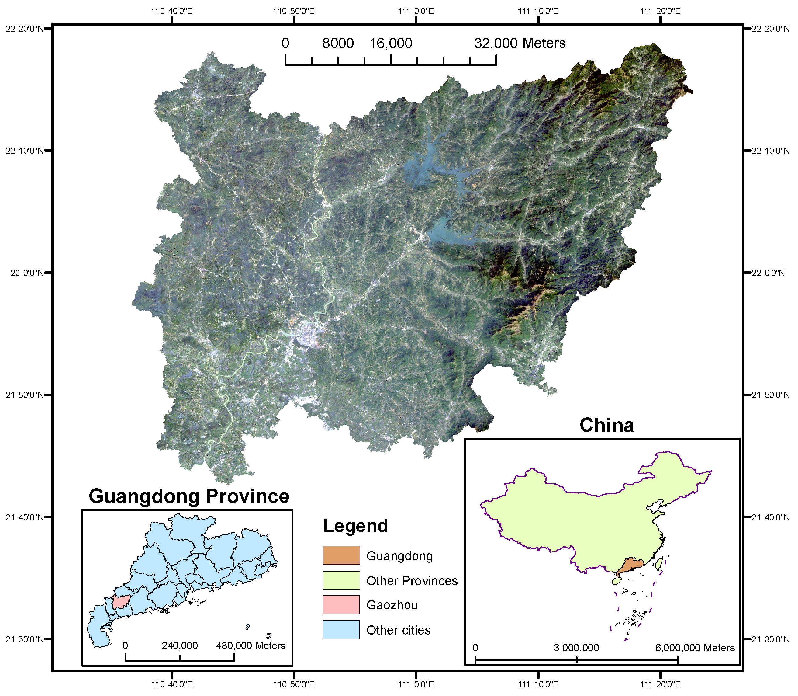
Figure 1. Landsat 8 remote sensing image of Gaozhou, Guangdong, China.
Agriculture 13 01541 g001
Figure 2. Map of the distribution of soil sampling points in the study area.
Agriculture 13 01541 g002
Figure 3. Spatial distribution mapping of environmental variable values in the study area. (a) TPI (positive and negative values indicate ridges and valleys, respectively). (b) TWI (a higher value indicates a higher potential humidity). (c) Aspect (aspect is expressed in positive degrees from 0 to 360, measured clockwise from north, and −1 indicates flatness). (d) Profile curvature (positive values indicate a raised terrain, and negative values indicate a depressed terrain). (e) Slope (the range is 0–90, with higher values indicating a steeper terrain). (f) Plane curvature (positive values indicate a raised terrain, and negative values indicate a depressed terrain). (g) Altitude. (h) Surface fluctuation (this variable reflects the height from the surface of the wind speed profile where the wind speed is zero; a higher value indicates a rougher surface). (i) Average annual temperature. (j) Average annual precipitation. (k) EVI.
Agriculture 13 01541 g003
Figure 4. Illustration of the structure of the Random Forest spatial interpolation model.
Agriculture 13 01541 g004
Figure 5. Illustration of the truncation line analysis method.
Agriculture 13 01541 g005
Figure 6. Mapping results of AP based on four spatial interpolation models.
Agriculture 13 01541 g006
Figure 7. Map of land use of the study area (obtained by the imagery of Landsat 8).
Agriculture 13 01541 g007
Figure 8. Illustration of the spatial variation of AP.
Agriculture 13 01541 g008
Figure 9. Three truncation lines that pass through the typical region from different directions.
Agriculture 13 01541 g009
Figure 10. Trend of the normalized values of elevation, EVI, and P on Truncation Line 1.
Agriculture 13 01541 g010
Figure 11. Trend of the normalized values of elevation, EVI, and P on Truncation Line 2.
Agriculture 13 01541 g011
Figure 12. Trend of the normalized values of elevation, EVI, and P on Truncation Line 3.
Agriculture 13 01541 g012
Table 1. RMSE results obtained by the four spatial interpolation models (two decimal places reserved).
ModelRMSE
RF32.01
OK32.08
RBF33.08
IDW32.74
Table 2. Importance of impact factors based on RF (importance ranking in parentheses).
Environment VariablesTPITWIAspectProfile CurvatureSlopePlane Curvature
importance31,970.42 (6)31,555.20 (7)28,539.34 (11)30,073.59 (10)32,466.85 (5)30706.98 (9)
Environment VariablesAltitudeSurface FluctuationAverage Annual TemperatureAverage Annual PrecipitationEVI
importance35,362.74 (2)31,330.63 (8)33,080.58 (4)33,367.12 (3)37,989.11(1)
Disclaimer/Publisher’s Note: The statements, opinions and data contained in all publications are solely those of the individual author(s) and contributor(s) and not of MDPI and/or the editor(s). MDPI and/or the editor(s) disclaim responsibility for any injury to people or property resulting from any ideas, methods, instructions or products referred to in the content.