Abstract
Peanuts are prone to insect damage, breakage, germination, mildew, and other defects, which makes the quality of peanuts uneven. The difference in peanut pod quality makes the price and economic benefit also have a big difference. The classification of peanut pods according to quality is an important part of improving the product grade and market competitiveness. Real-time, accurate, and non-destructive quality detection of peanut pods can effectively improve the utilization and commercial value of peanuts. The strong subjectivity of manual detection and the low efficiency and low accuracy of mechanical detection have caused considerable wastage. Therefore, the present study proposed a new convolutional neural network for the peanut pod quality detection algorithm (PQDA) based on an improved ResNet. Compared to previous models, this model is more practical with high accuracy, lightweight, and easy nesting. Firstly, the detection and classification effects of ResNet18, AlexNet, and VGG16 are compared, and ResNet18 was determined to be the best backbone feature extraction network for model training. Secondly, three models were designed to optimize and improve the algorithm. The KRSNet module was added to the algorithm to make the model lightweight. The CSPNet module was added to the algorithm to improve the learning efficiency of each feature layer. The Convolutional Block Attention Module (CBAM) was added to the algorithm to improve its ability to capture more feature information about peanut pods. The experimental ablation results show that the precision of the improved model PQDA reaches 98.1%, and the size of parameters is only 32.63 M. Finally, the optimized model was applied to other peanut pod varieties for generalization experiments, and the accuracy reached 89.6% and 90.0%, indicating the effectiveness of the proposed peanut pod quality detection model. Furthermore, the model is suitable for deployment on embedded resource-limited devices, such as mobile terminals, to achieve the real-time and accurate detection of peanut pod quality.
1. Introduction
Peanuts are one of the most important cash crops in the world and are cultivated all over the world. China is the largest peanut producer in the world, with a planting area of over 5 million hectares, accounting for approximately 40% of the world’s total production [1]. Peanut pod quality detection is one of the key technologies for peanut storage, deep processing, and improving product grade and added value. However, peanuts are prone to insect damage, breakage, germination, mildew, and other defects in the process of growth, fruit–seedling separation, transportation, and storage, which makes peanut quality uneven. Even moldy peanuts produce carcinogenic substances such as aflatoxin, which seriously threatens people’s health [2]. Different qualities of peanut pods have different uses, different prices, and different economic benefits. Quality detection before sale, reprocessing, and export can enhance the value of peanut pods and achieve the multi-channel utilization of products. Achieving consistent peanut pod quality through quality detection is of great significance for safe storage and reprocessing, improving product grade and market competitiveness. At the same time, in the import and export trade, there are strict regulations on the quality of peanut pods. The industrialization and scale of peanuts also make people have higher requirements for peanut pod quality grade and detection efficiency. Traditional manual sorting is subjective, inefficient, and costly, while mechanical sorting has poor real-time performance and has difficulty ensuring classification accuracy. Machine vision technology provides a non-contact automatic detection method with the advantages of being real-time, efficient, objective, and relatively low in cost, and it has been widely applied in the field of food quality inspection [3]. Designing a fast, accurate, economical, and intelligent peanut pod quality detection algorithm that is suitable for embedding into small hardware devices for online detection has important scientific and social significance.
In the agricultural field, machine vision has been widely applied in plant leaf disease and pest detection [4,5,6,7,8], weed detection [9], seed-grading detection [10,11,12,13], and fruit-maturity detection [14,15,16]. Meng et al. [17] proposed a convolutional neural network classification model based on a self-attention mechanism to improve the accuracy in distinguishing between crop species in fields using spectral canopy information, with an accuracy of 99.93%. Yuan et al. [18] proposed a fine-grained image classification model for the chrysanthemum category based on transfer learning and VGG16, with an accuracy of 98.15%. Bhupendra et al. [19] developed a machine vision system that proposed a convolutional neural network (CNN) model-based classification of seven types of preprocessed rice grains, achieving an overall classification accuracy of 98.37%. Dogan et al. [20] studied the mixed structure of Extreme Learning Machine (ELM) and GoogLeNet transfer learning. The proposed SSA-ELM model successfully classified 14 different types of dry beans, with a success rate of 91.43%. Zhao et al. [21] proposed a multiscale feature fusion network to effectively extract rich strawberry disease features. The results showed that it could detect healthy strawberries and seven kinds of strawberry diseases with high accuracy and speed. Huang et al. [22] studied lightweight models to implement soybean seed classification, including three standard CNN models and three lightweight models. These models can be imported to resource-limited platforms to make the detection process more efficient. Wang et al. [23] designed a Faster R-CNN model improved with (a residual network) ResNet-50 as an algorithm for the detection of tomato maturity. Its average detection accuracy was 96.14% in branch occlusion, fruit overlap, and illumination effects. Jia et al. [24] combined a residual network (ResNet) with a densely connected convolutional network (DenseNet) to obtain the region where apples were located, with an accuracy of 97.31% and a recall of 95.70%. Zhang et al. [25] proposed a new high-throughput method combining VGG-16 and Resnet-50 dual-path convolutional neural networks to screen maize ears in a real seed production plant with an average classification accuracy of 97.23%.
At present, deep learning has been widely applied in agriculture. Convolutional neural network technology has been applied in the actual agricultural environment, such as image classification [26,27,28], object detection [29,30,31,32], and image segmentation [33,34,35,36,37], with good performance. Therefore, the study of peanut kernels and peanut pods in this field has attracted the attention of many scholars. Zou et al. [38] studied classification algorithms for different peanut varieties based on hyperspectral imaging technology. The designed XGBoost and LightGBM classification models have an accuracy of 99.33%. Zhang et al. [39] proposed a defect-recognition system for peanut kernel quality based on machine vision and adaptive convolutional neural networks. Based on this system, an average recognition rate of 99.7% was achieved for common defects, including mold, crushing, and shriveling. The classification of peanut kernels is generally applicable to the quality test of peanut seeds and so on, which has limited application. In contrast, the intelligent screening of peanut pods is more practical and universal. Ni et al. [40] designed an improved AlexNet to identify and classify 13 different varieties of peanut pods. The highest accuracy of this improved model reached 88.76%, with an average accuracy of 87.73%. Yang et al. [41] obtained peanut pod images of 12 varieties by scanner. Meanwhile, the improved deep convolutional neural network VGG16 was applied to the recognition and classification task of the peanut data set, with an average accuracy of 96.7%. In the related research on peanut pods, there are more studies on the detection of pod varieties and less research on pod quality. However, the regional planting of peanuts uses a fixed variety, so the practicality of variety identification is not significant. Zhang et al. [42] proposed a method of peanut pod grade recognition based on a convolutional neural network of transfer learning. Through the transfer of the AlexNet convolution layer, the peanut pod classification accuracy rate in five grades reached 95.43%. Deng et al. [43] used a support vector machine (SVM) and K-means algorithm for variety recognition and lineage clustering by extracting size, shape, color, and texture features. The recognition rate of the SVM model is over 90%.
Overall, the current research on peanut pod quality detection has cumbersome sampling, low accuracy, poor real-time, and large capacity of the algorithm is not easy to embed in mobile devices, which makes the algorithm limited to the theoretical level and unable to be widely applied.
Thus, in response to the above issues in current research on peanut pod quality detection, this study proposed a detection algorithm based on the improved ResNet18. Aiming at the quality detection of peanut pods, a low-cost, high-accuracy, real-time, and lightweight peanut pod detection algorithm was studied, which was suitable for embedding into hardware equipment. The key findings and highlight the specific goals of the research are summarized as follows:
- We established a low-cost data acquisition system that captured RGB images through industrial cameras. Also, we established a standardized peanut pod quality dataset, including six categories: normal, insect pest, mildew, single fruit, damaged, and sprouted;
- A peanut pod quality detection model PQDA was established to solve the basic problems at present. The algorithm had the characteristics of high accuracy, fast detection, and small model size;
- The model was evaluated by a self-established peanut pod database, and the generalization experiment was carried out. We verified the generalization ability of the model and provided a reference for the precise grading of other agricultural products.
2. Materials and Methods
2.1. Materials
2.1.1. Dataset Acquisition
In this study, the peanut pod of Xiaobaisha 1016 was taken as the research object, and the original data images for the peanut pod quality classification experiment were taken by ourselves. The peanuts were collected from the peanut base in Tancheng County, Linyi City, Shandong Province, China. After preliminary screening, a total of about 1000 peanut pods of each variety were collected. The collected peanut pods were artificially classified into 6 categories: normal, insect pest, mildew, single fruit, damaged, and sprouted. The RGB images of Xiaobaisha 1016 were captured using a machine vision experimental rack combined with a MOKOSE c100 camera, with an initial pixel resolution of 1920 × 1080. In order to show the characteristics of each peanut pod in an all-around way, a single peanut pod was photographed from different directions, and then the characteristics of the peanut were magnified by cropping. A total of 1360 images were obtained, including 276 normal peanuts, 210 insect pest peanuts, 223 damaged peanuts, 206 moldy peanuts, 218 sprouted peanuts, and 227 single fruit peanuts. The quantity of peanut images in each category of the self-built peanut pod dataset is shown in Figure 1.

Figure 1.
Examples of peanut pod images: (a) normal image; (b) insect pest image; (c) sprouted image; (d) mildew image; (e) damaged image; and (f) single fruit image.
2.1.2. Data Augmentation
Data augmentation could improve the outcomes and enhance this study’s ability. To further ensure dataset availability and generalization ability, data augmentation was used for image expansion. According to the characteristics of each kind of peanut, different kinds of images were appropriately enhanced, such as adding Gaussian noise, brightness darkening, and vertical symmetry transformation. Figure 2 illustrates the effect of peanut pods after a certain data augmentation. The peanut pod images were expanded to a total of 4080. Detailed information on the self-made peanut pod dataset is shown in Table 1. The dataset was divided into a training set and a test set in a ratio of 9:1 randomly. All images in the dataset were uniformly resized to 224 × 224 before being input into the model.

Figure 2.
Examples of image preprocessing operations (brightness darkening (b), Gaussian noise (c), and vertical (d) operations are performed on the original picture (a), respectively).

Table 1.
Category name and quantity of peanut pod quality dataset.
2.2. Methods
2.2.1. Introduction to ResNet18
ResNet [44] network is a widely used algorithm for image classification and recognition tasks. The residual block structure proposed in the network effectively solved the problems of gradient vanishing or exploding due to the deepening of network layers. The specific structure of the residual block is shown in Figure 3, and a single residual block can be expressed as:
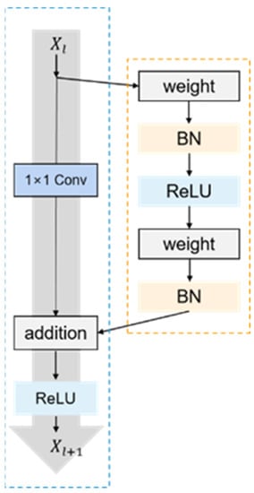
Figure 3.
Residual structure diagram.
The residual block is composed of identity mapping and residual parts. Figure 3 shows the identity mapping on the left (in the blue box) and the convolution part on the right (in the yellow box). denotes a residual module, typically consisting of two or three convolution operations. In the convolutional network, if the feature and have different sizes, 1 × 1 convolution should be used to reduce or raise the dimension. In this case, the residual block can be expressed as:
where , is a 1 × 1 convolution operation, used to raise or reduce dimensions.
As shown in Figure 4, the ResNet18 structure consists of 8 sets of residual blocks, an initial convolutional layer, and a fully connected layer. Each set of residual blocks has a 2-layer convolutional structure, with a total of 18 weight layers.

Figure 4.
ResNet18 structure diagram.
The initial input was a 224 × 224 GRB three-channel image, and the output was the number of peanut pod quality classification kinds. The first convolutional layer used 7 × 7 kernels with the stride step of 2, so the number of channels became 64, and the size was 112 × 112. Then, after the max-pooling layer with 3 × 3 kernels and 2 stride steps, the number of channels remained unchanged, and the size was reduced to half of 56 × 56. Finally, we entered the residual part, which had 8 residual blocks, each of which contained 2 convolutional layers with 3 × 3 kernels. At last, the output features were connected to the fully connected layer through the adaptive average pooling layer after downsampling. The probability of each category was calculated by the Softmax layer. The network structure parameters of ResNet18 are shown in Table 2.

Table 2.
Description of output sizes for each layer in ResNet18.
2.2.2. KRS-ResNet18 Design
In order to make the model easy to embed into resource-limited embedded devices, the KRS lightweight method was added to modify the model structure. This would further reduce the number of model parameters and reduce their complexity. The modification of the KRS lightweight method to the model mainly included three aspects: adjusting the convolution kernel, and optimizing the identity mappings and the residual blocks.
The first convolution layer of ResNet18 has a convolution kernel of size 7 × 7 and a stride step of 2. The formula for the forward calculation of the image receptive field is as follows:
Equations (3) and (4) are the calculation formulas of the receptive field of the initial convolution layer and the intermediate convolution layer, respectively. Where is the convolution kernel, denotes the convolution step size, denotes the convolution kernel size of the nth layer, denotes the step length of each previous layer, and denotes the effective receptive field of the previous layer. By calculating the receptive field, it can be seen that the receptive field of one 7 × 7 convolution kernel is the same as that of three 3 × 3 convolution kernels, with both being 7. After using two kinds of convolution kernels, the size of the input image changed from 224 × 224 to 218 × 218. But the total number of parameters used in a 7 × 7 convolution kernel is 49× Channels, while the total number of parameters used in three 3 × 3 convolution kernel is 27× Channels. The number of model parameters can be reduced by changing the size of the convolution kernel. The specific conversion is shown in Figure 5a.
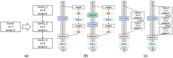
Figure 5.
KRS-ResNet18 structure: (a) replace convolutional kernel; (b) optimize residual blocks; (c) replace residual block convolutional structures.
When the output of identity mappings of the residual block in the model is different from the output of the residual part, it is usually necessary to modify the input size by adding a convolutional layer with a convolutional kernel of 1 × 1 stride step size 2 to the identity mapping so that the two outputs of the residual block can be summed. It is thus considered that an average pooling layer can be added to the identity mapping instead of the original 1 × 1 convolutional layer. The newly added average pooling layer can further simplify the feature map, reduce the complexity of the network, and prevent overfitting. The specific modified structure is shown in Figure 5b, with the original structure on the left and the optimized structure on the right.
In the original ResNet18, the convolution of the residual part of the residual block is composed of 2 convolutional layers with 3 × 3 convolutional kernels. To further reduce the number of model parameters, the convolutional structure here was modified, and two convolutional layers with 3 × 3 convolution kernel were modified into three convolution layers with 1 × 1, 3 × 3, and 1 × 1 convolution kernel, respectively. The original downsampling has been realized by the improved 3 × 3 convolution. Although the improvement will lead to the weakening of model learning ability, it can offset the decrease of its accuracy and greatly reduce the number of model parameters when combined with other overall optimization, so as to achieve the overall optimization effect. The specific modified structure is shown in Figure 5c. The left picture is the original structure, and the right picture is the improved structure.
2.2.3. CSP-ResNet18 Design
In order to solve the impact of reducing the number of parameters on the accuracy of the model, the cross-stage partial network (CSPNet) adapted to the KRS lightweight method was added to the network. The CSPNet was applied to strengthen the real-time model while increasing model accuracy, decreasing runtime network computation and memory traffic, and further increasing CNN’s learning capabilities. The main idea of CSPNet is to segment a network feature map and process it in different stages. The feature map is divided into two parts; one part was used for the calculation of the current stage, while the other part was used for cross-stage transmission.
This cross-stage information transmission could better retain high-level information about the feature map. Combining with CBAM, it not only compensated for the decrease in accuracy caused by a reduction in parameter quantity, but also further improved the accuracy of the model compared to the original ResNet18. We integrate the CSPNet algorithm into the original ResNet18 structure shown in Figure 6a. The feature map segmentation operation of CSPNet was added between each residual block in ResNet18. The input feature map was divided into two parts, one for the current Residual Block calculation and the other for cross-stage transmission. When the output sizes of the two parts of the feature map were different, the channels of the cross-stage transfer part were adjusted by a 1 × 1 convolution kernel. The two parts of feature maps were computed in parallel, which can reduce the repetitive operations of feature maps and improve computational efficiency to a certain extent. Then, the two parts of the feature map were merged through concatenation to form the output feature map of the current stage. The complete CSP-ResNet18 structure is shown in Figure 6b.
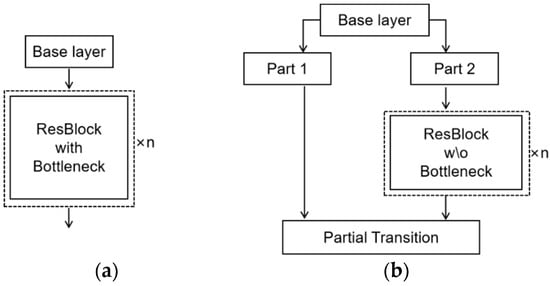
Figure 6.
Comparison between the original network structure and the improved network structure: (a) structure of ResNet18; (b) structure of CSP-ResNet18.
2.2.4. CBAM-ResNet18 Design
To better extract the quality characteristics of various types of peanut pods, CBAM [45] was added to the ResNet18 for optimization. CBAM attention mechanism is a lightweight attention module for convolutional neural networks, which includes two main parts: channel attention mechanism and spatial attention mechanism. These two attention mechanisms are independent of each other, but can be connected together to help the model capture more important features.
The goal of the channel attention mechanism is to explore the relationships between different channels. It highlights feature channels that are more important to the task by assigning weights to each channel. The structure of the channel attention mechanism is shown in Figure 7a. Firstly, the input feature map was subjected to global average pooling (GAP) and global max-pooling (GMP). The above operation compressed the feature map in the spatial dimension and generated channel description features for average and maximum response, respectively. Next, the output of GAP and GMP were, respectively, passed through a shared weighted multi-layer perceptron (MLP). MLP typically consists of two fully connected layers, with the activation function ReLU in between. This step was to further learn the relationship between channels, add the MLP output elements, and then map the results to the (0,1) range through the Sigmoid activation function as the channel attention weight. Finally, the channel attention map was multiplied by the input feature map for adaptive optimization to obtain a weighted feature map. The specific calculation process of channel attention was as follows:

Figure 7.
CBAM structure diagram: (a) channel attention structure; (b) spatial attention structure.
In the equation, denotes Sigmoid function, , . The weights of MLP were shared by and , was as preceded by ReLU activation function, and and represented average and max-pooling characteristics, respectively.
The purpose of the spatial attention mechanism was to explore the relationships between spatial positions in feature maps. It assigned weights to each spatial position to highlight the spatial regions that were more important to the task. The structure of the spatial attention mechanism is shown in Figure 7b. Firstly, the input feature map was subjected to average pooling and max pooling along the channel dimension, and the average and maximum value aggregation of spatial positions were performed. Next, the average and maximum pooled outputs were concatenated on channel dimensions. Then, the number of channels was adjusted by a convolutional layer with an input channel number of 2, an output channel number of 1, and a convolutional kernel size of 7 × 7 to further learn the relationship between spatial locations. The output of the convolution layer maps the result to the range of (0, 1) through the Sigmoid activation function as the spatial attention weight. Finally, the spatial attention weight was multiplied by the input feature map to obtain the weighted feature map. The specific calculation process of spatial attention was as follows:
In the equation, denotes the Sigmoid function, denotes a 7 × 7 sized convolution kernel, , . and denote the average pooling feature and the max-pooling feature across channels, respectively. The CBAM attention mechanism used in this study was formed by the channel attention mechanism and the spatial attention mechanism in tandem. The specific structure is shown in Figure 8, where the input feature map , . Firstly, a one-dimensional channel feature map Mc, was generated by the channel attention module, and then a two-dimensional feature map Mc, was generated by the spatial attention module.
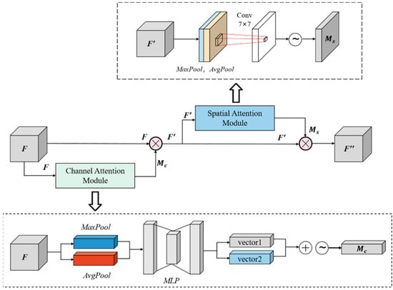
Figure 8.
Convolutional block attention module.
The whole process is summarized below. The channel feature map Mc was multiplied by the input feature map element by element to obtain . Then, was used to generate the spatial feature map through the spatial attention module; after that, Ms was multiplied by element by element to obtain the final output .
The structure of CBAM-ResNet18 is shown in Figure 9. The CBAM module was added to the residual part of the residual block. The feature map obtained by convolution in the residual part before was the input of the CBAM module. The feature map was processed by the CBAM module, and the weighted features were output. We replaced the original convolutional feature map and added it to the identity mapping of the residual block to form the ResBlock-CBAM. The original ResBlock structure was substituted with the Resblock-CBAM structure when setting up the ResNet18 network. This successfully added the CBAM attention mechanism to form the new network CBAM-ResNet18.
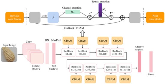
Figure 9.
CBAM-ResNet18 structure.
2.2.5. PQDA Module Design
Integrating the three network models above, we designed a new peanut pod quality detection algorithm named “PQDA”. Based on the ResNet18 network, this model was further reduced by KRS lightweight, CBAM attention module, and CSPNet were added to enhance feature learning ability and reduce model computation and memory storage.
The structure of the PQDA is shown in Figure 10. Firstly, the input feature map was divided into two parts for parallel computation according to the CSP-ResNet18 structure. Then, the residual block was performed using the KRS lightweight method, modifying the identity mapping and residual parts to reduce the number of model parameters. Next, the CBAM attention mechanism was added to this part, and the output feature graph of the convolutional structure was modified as its input. The cross-stage transfer part used a 1 × 1 convolution kernel to adjust the number of channels. Finally, the two parts of the output were concatenated and merged according to the CSPNet concept to form the current stage output feature map. We replaced the newly generated convolutional feature map with the original ResNet18 convolutional feature map generated by residual blocks for forward propagation. The rest parts were built according to the original ResNet18 network, thus completing the PQDA.
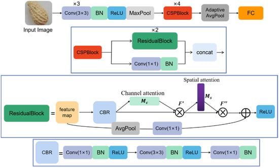
Figure 10.
PQDA model structure diagram.
2.3. Evaluation Indexes
In evaluating the performance of classification models in detecting peanut pod quality in this study, accuracy, precision, recall, and F1-score were taken as evaluation Indexes. They consist of four components: true positives (TP), false positives (FP), true negatives (TN), and false negatives (FN). The precision rate measures the proportion of properly predicted samples, while R (Recall) refers to the proportion of the predicted positive samples in the actual positive samples. The recall rate reflects the model’s ability to identify positive samples. That is to say, recall (or True Positive Rate) is calculated by dividing the true positives by anything that should have been predicted as positive. The F1 score is a comprehensive performance index expressed as the harmonic mean of recall and precision, thereby achieving an optimal outcome.
2.4. Experimental Environment and Parameter Settings
The computer parameters for model training are Intel(R) Core(TM) i9-10920X CPU with 3.50 GHz, 64.0 GB RAM, and NVIDIA GeForce RTX 2080 Ti graphics card with 11 GB video memory. The system is Windows 10 Professional operating system, Python version 3.9.7, Cuda 10.0, and PyTorch framework is selected for program writing, version PyTorch 1.12.1, with Pycharm software for data processing and result visualization operations.
This research on peanut pod quality classification was a single-label and multi-classification problem, and the image size was uniformly adjusted to 224 × 224 before input into the model. In order to have a faster training speed, we set the data loader to load 10 data for each batch. The learning rate was set to 0.0001. For forward propagation, Cross Entropy Loss was used to calculate the loss. The cross-entropy loss function was often applied in deep learning classification tasks and was calculated as follows:
where was the number of samples in the current batch, was the number of label categories, was the true distribution, and denoted the network output distribution. The optimizer used Random Gradient Descent (SGD) when the parameters were updated by backpropagation. The formula was as follows:
Denoted the weight parameter to be updated as , denoted the learning rate, and was the gradient of the loss function with respect to . Set the batch size of the training to 32 and the epoch to 400. Finally, the Softmax layer was used to output the specific category probability. Softmax was shown as follows:
where referred to the true probability that the target belonged to the class . Instead of scoring image categories directly, the Softmax layer estimated a probability for each category, that was, the probability that the input image belonged to each category. Its function was to normalize the corresponding output components of each category so that the sum of each component was 1.
3. Results
3.1. Performance Comparison between Different Networks
Aiming at the research of peanut pod quality classification in this subject, the performance of the classic ResNet18, Alexnet, and Vgg16 was compared at first. By comparing the three models, the size of the parameters of ResNet18 was 42.65 MB, which was a lightweight model. Alexnet was relatively simple, including 5 convolutional layers and 3 fully connected layers, but each convolutional layer contained a large number of convolutional nuclei, so the size of the model reached 217.55 MB. The depth of Vgg16 was further enhanced, which had 13 convolutional layers and 3 fully connected layers. Each convolutional layer was equipped with a different number of convolution kerns of 3 × 3 size for feature extraction, and the size of model parameters was 512.26 MB. Reducing model size helped reduce memory requirements and computing costs, which greatly improves performance.
3.2. Optimization Effect of Improved Model
3.2.1. CBAM-ResNet18
Each residual block in ResNet18 was embedded into the CBAM module to form the network CBAM-ResNet18. The feature maps output by each convolution layer without and after improvement are shown in Figure 11. For CNN structure, its shallow convolution mainly learned simple features such as edges and lines of images, while the deep convolution paid attention to more complex specific features to realize the recognition and classification of images. The damaged quality peanut pod sample was taken as an example (from left to right, from top to bottom) to output the layer-by-layer feature map. Figure 11b was the convolutional feature map output by CBAM ResNet18. Compared to Figure 11a, the shallow convolution in Figure 11b extracted the overall contour features of peanut pods more clearly, and the shape of peanut pods was basically preserved for feature learning. In the deep convolution section (especially the last 5 feature maps), the model’s focus in Figure 11a did not focus on the damaged features of peanuts. However, the features learned from Figure 11b were more concentrated in the damaged area, indicating that the model has begun to pay more attention to the damaged characteristics of peanuts, thus achieving feature separation and recognition. After adding the CBAM module, more emphasis was placed on preserving overall features and extracting local features. As the network deepens, the specificity of feature points gradually increases.
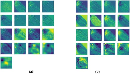
Figure 11.
Comparison of feature maps: (a) ResNet18 hidden feature map; (b) CBAM-ResNet18 hidden feature map.
The Avg_loss curve is shown in Figure 12a. As shown in the figure, the overall curve tended to be smooth, the model became stable with little loss after about 150 iterations, and the model converged faster. There was almost no obvious fluctuation in the later period, which indicated that the network stability was good.

Figure 12.
Comparison of three optimization improvement loss curves: (a) the loss of CBAM-ResNet18; (b) the loss of KRS-ResNet18; (c) the loss of CSP-ResNet18.
Compared with the original ResNet18, the stability of the model was enhanced. The accuracy was further improved, reaching 98.7%, the R (Recall) was 98.8%, the P (Precision) was 98.7%, and the F1-score was 98.8%. Each evaluation index had improved compared with the original. Similarly, as a lightweight module, CBAM had almost no change in the number of model parameters after it was embedded into ResNet18. Overall, the model performance has been optimized and enhanced.
3.2.2. KRS-ResNet18
The reduction of model parameters often leads to a decrease in model performance. This article used the KRS lightweight method combined with the ResNet18 to achieve the goal of greatly optimizing model parameters with a small sacrifice of accuracy. The original ResNet18 had a parameter size of 42.65 MB, but with the addition of KRS, the parameter size decreased to 24.04 MB, resulting in a decrease of approximately 43.6%. The evaluation of the improved model maintained a high level, as shown in Figure 12b, with the Accuracy of 94.9%, the R (Recall) of 94.9%, the P (Precision) of 95.0%, and the F1-score of 94.8%. Compared with Figure 12a, the curve showed small-scale oscillation, the bending amplitude became larger, the convergence effect decreased, and the loss became smaller and approached 0 after about 300 iterations. Simply reducing the size of model parameters would have a slight impact on the model performance, and this method needed to be combined with other improved methods to reflect its optimal optimization effect.
3.2.3. CSP-ResNet18
In this study, the CSPNet network was used to optimize the performance degradation caused by reducing the number of parameters. Compared with other models, adding the idea of feature map segmentation of the CSPNet network to the lightweight model with fewer parameters can result in more significant optimization effects. After adding the CSPNet network to the ResNet18 model, the model parameter quantity increased to 50.56 MB, and various evaluation Indexes have improved obviously. The memory flow occupied by the model during training decreased, and the model training time also decreased. After 400 training, the CSP-ResNet18 model achieved an Accuracy of 99.0%, an R (Recall) of 99.0%, a P (Precision) of 99.1%, and an F1-score of 99.1%. The Avg_loss curve of this model is shown in Figure 12c. The first 100 training curves were relatively smooth, and the later curve oscillated greatly, indicating that the stability of the model needed to be improved. It could be combined with the CBAM module to improve the stability of the model. The final model loss value was closer to 0 than the previous two, and the accuracy was improved by more than 1%, indicating that the optimization effect was significant.
The loss curves of these three classic networks are shown in Figure 12, and the accuracy curves are shown in Figure 13. It was seen from the figure that the accuracy of ResNet18 was relatively highest in the three models. The results of the other evaluation Indexes are shown in Table 3 below. Based on all the evaluation Indexes and model size, it could be concluded that the performance of the ResNet18 was relatively superior in this research on peanut pod quality detection.
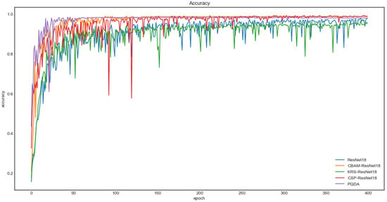
Figure 13.
Accuracy curve of the training set for different improved networks.

Table 3.
Comparison of evaluation index for backbone network selection.
3.3. Effect of the PQDA Model
The new peanut pod quality detection model named PQDA was based on the ResNet18 network and optimized from two aspects: improving accuracy and reducing parameter quantity. In terms of reducing the size of model parameters, using KRS lightweight method to modify the structure, the size was reduced from 42.65 MB to 32.63 MB, reducing by approximately 23.5%. In terms of improving the accuracy of the model, introducing the CBAM attention module and the feature map segmentation of CSPNet to improve the model learning ability, the accuracy of the model was further improved. Compared with the original with the reduced number of parameters, from 97.8% to 98.0%, the convergence speed of the model was accelerated, and the accuracy curve was more stable. The PQDA-ResNet18 model achieved an Accuracy of 98.0%, an R (Recall) of 98.1%, an accuracy rate of P of 98.1%, and an F1-score of 98%.
Figure 13 illustrates the accuracy curves of the five network learning processes described in Table 4. The graph results were presented under the same learning rate and optimizer conditions. CSP-ResNet18 has improved the accuracy of the model, while CBAM-ResNet18 has improved the robustness of the system. Although KSP-ResNet18 had slightly poor stability, its main role in optimizing the entire model was to lighten the weight and reduce the size of the parameters. In summary, the accuracy curve of PQDA has been greatly improved compared with the original model, and it is suitable for deployment in field equipment.

Table 4.
Results of ablation experiment performance evaluation index.
Table 4 shows the evaluation indexes and parameters of the five models. It indicates that the accuracy and other indexes of the model are higher than the original ResNet18 after the CBAM attention module and CSPNet are integrated. After using KRS lightweight method, the number of model parameters decreased obviously. By comprehensive comparison, PQDA has the best performance.
3.4. Model and Algorithm Test
The confusion matrix is a visual tool for evaluating the performance of classification models. It is used to help one understand the accuracy and error type of the model in each category. The confusion matrix shows the correspondence between the actual category and the predicted category. The model performance metrics, such as accuracy and precision, can also be derived based on it. For multi-classification problems, the confusion matrix is an N × N matrix, where N is the number of categories, and the diagonal of the matrix indicates that the predicted categories are consistent with the actual categories, and the prediction is correct.
The original network, the three improved networks, and the optimized network were trained on the self-built peanut pod data set. The confusion matrix of the whole network was predicted by using the test set, as shown in Figure 14. In the CSP-ResNet18 test performance, only four labels were predicted incorrectly, indicating that the algorithm is outstanding in improving accuracy. In the confusion matrix of CBAM-ResNet18, only 5 labels were predicted incorrectly, indicating that the algorithm was effective in feature extraction. However, the KRS-ResNet18 had slightly more major prediction errors because the main purpose of introducing this algorithm was to reduce the number of parameters and make the model lightweight. In the designed PQDA confusion matrix, three sprouted peanuts, one normal peanut, and two damaged peanuts were wrongly predicted to be single-fruit peanuts. Two damaged peanuts were predicted to be moldy peanuts and insect peanuts, respectively. It had a false prediction rate of just 1.9%. The overall prediction result was promising.

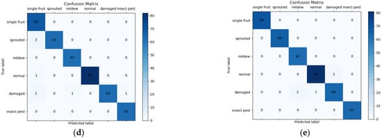
Figure 14.
Comparison of confusion matrix of models: (a) Confusion matrix of ResNet18; (b) Confusion matrix of KRS-ResNet18; (c) Confusion matrix of CSP-ResNet18; (d) Confusion matrix of CBAM-ResNet18; (e) Confusion matrix of PQDA.
4. Generalization Experiments
We collected peanut pods of Tsinghua 6 and Tianfu 11 at the Peanut Experimental Base of the agricultural college. Next, we self-established validation datasets for them, respectively. Qinghua 6 and Tianfu 11 peanut pods were selected for generalization experiments to test the generalization ability of the model. Compared with Xiaobaisha 1016 peanut, the overall pods of Qinghua 6 peanut are larger and fuller, and the pods of Tianfu11 peanut are thinner and smaller. A total of 480 images were taken of each variety of peanut, with 80 images of each of the six classifications. The PQDA was utilized to predict, using the primary weight with the least training loss as the prediction weight. The confusion matrix was output to evaluate the model with various evaluation Indexes.
Figure 15 shows that in the confusion matrix of Qinghua six peanut pods, eight damaged images were predicted to be normal images, and seven mildew images and sprouted images were predicted incorrectly with each other. The results indicated that PQDA was not very accurate in the extraction of moldy and germinating features of this type of peanut for Qinghua 6. The accuracy of the design model applied to this category reached 89.6% (as shown in Table 5). In the confusion matrix of Tianfu 11, 11 normal images were incorrectly predicted as single fruit images, which was slightly worse than other categories. Other types of prediction had a good effect, and the accuracy of PQDA applied to this category reached 90% (as shown in Table 5). It is shown that the optimization model proposed in this paper has good generalization ability and can be extended to identify different kinds of peanut pod quality detection. At the same time, it provides a reference for expanding the application range of the model.
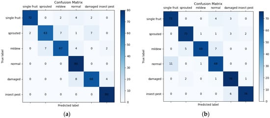
Figure 15.
Confusion matrix of the generalization experiment: (a) Confusion matrix of Qinghua 6; (b) Confusion matrix of Tianfu 11.

Table 5.
Results of generalization experiment for other peanut varieties.
5. Discussion
In this study, we proposed a peanut pod quality detection method based on improved ResNet. The algorithm took ResNet18 as the backbone network, and integrated the CBAM attention mechanism, KRSNet, and CSPNet networks. The accuracy, lightweight and detection speed have been improved up to a point. Evaluated with the self-built dataset, accuracy, recall, precision, and F1 score increased by more than one percentage point with a 23.5% reduction in parameter size. The results obtained in this study were compared with current studies in the literature on the application of deep learning models to peanut pod detection. Compared with Zhang et al. [39], who improved the peanut pod level recognition model by transferring AlexNet convolutional layer, the peanut pod level recognition model (Penut_AlexNet model, PA model) was constructed, and the accuracy of peanut pod classification and recognition in five levels was 95.43%, Recall of 95.422%, F1 score of 96.074%. Compared with it, the PQDA proposed in this study (each index in Table 4) is 2.038%, 2.678%, and 1.926% higher than it, respectively, and the model size is less than one-fifth of it.
In the algorithm proposed in this study, data acquisition could be completed using an industrial camera with a stand, and the peanut pods did not need to be regularly placed. As a cost-effective quality detection tool, RGB images and deep learning could be successfully applied to peanut pod quality detection in industry and agriculture. The literature [35] used hyperspectral imaging to study the classification algorithm of different peanut varieties, and the literature [37,38,39,40] used the regular placement of scanners for data acquisition, which limited the practicality of the model. Secondly, in order to improve the ability to capture more features of peanut pods, the CBAM attention module was added. The KRSNet module was added to adjust the convolution kernel and optimize the residual block. The addition of the CSPNet module reduced the amount of network computation and memory size. The improved model maintained a better effect even after the lightweight. In addition, we conducted a generalization experiment in the other two varieties of peanut pod quality detection experiments, and the effect was good. These optimizations made the improved model have strong generalization ability and high practicability. At the same time, the parameter model was only more than 30 M, which was far smaller than similar research models. This provided a theoretical basis for deploying mobile devices to promote the development of intelligent agricultural machinery.
The method developed in this study was carried out for generalization. The experimental results were good, which can be applied to the quality detection for other varieties of peanut pods. Meanwhile, the system was a lightweight CNN model suitable for deployment on embedded devices such as Raspberry Pi 4B. In the future, GUI interfaces can run the trained model directly on the Raspberry PI. It can be developed to realize visual operation and facilitate the use of ordinary growers. In addition, the model can be called on embedded devices and equipped with screening devices in intelligent agricultural machines such as peanut combine harvesters to complete the classification and detection of different quality peanut pods. In summary, this algorithm lays the theoretical foundation for the future development of a quality detection system that can operate with low cost and high precision in industrial environments.
6. Conclusions
In this paper, a method of peanut pod quality detection based on the ResNet18 algorithm was proposed based on the images of peanut pods harvested in peanut base as the original data. A dataset of six classifications of peanut pods was established and expanded to 4080 sheets by data enhancement to improve the generalization ability of the model. By comparing three classical feature extraction networks, ResNet18 was chosen as the backbone network in this study with an accuracy of 97.8% and a reference quantity of 42.65 MB, which was obviously superior to other models. The CSPNet module adapted to the KRS lightweight method was added to improve the model accuracy and enhance the real-time model performance, and the model accuracy was 99.0%. The KRS lightweight module is embedded into the backbone network by replacing the convolutional kernel, optimizing the residual block, and replacing the convolutional structure of the residual block, which reduces the size of network parameters by about 43.6%. The CBAM module was integrated to carry out adaptive feature refinement along channel and space. The effectiveness of fusing the above three improvement methods was verified by ablation experiments, and the F1-score of the optimized model reached 98%, and the number of parameters was reduced by 23.5% compared with the original model. At the same time, generalization experiments were conducted, and the improved model was applied to other varieties of peanut pod quality detection, and the accuracy was also around 90% with high accuracy and high generalization ability. In addition, on the basis of maintaining excellent evaluation indexes, the model size of only 32.63 MB is suitable for the deployment of small, embedded devices, which provides reference and guidance for further development of real-time detection of peanut pod quality with hardware devices.
Author Contributions
Conceptualization, L.Y.; formal analysis, D.W.; investigation, C.W. and L.Y.; data curation, N.X.; funding acquisition, L.Y. and J.Y.; methodology, C.W.; writing—original draft, L.Y. and C.W.; writing—review, L.Y. and D.W.; visualization, C.W. All authors have read and agreed to the published version of the manuscript.
Funding
This research was funded by the National Key Research and Development Program “Research and Integration Demonstration of Light Simplified High Yield Technology for Soybean and Other Oil Crops” Project “Research and Development of Common Light Simplified High Yield Technology for Main Oil Crops” (2022YFD2300101) and Key Research and Development Plan of Shandong Province (Major Science and Technology Innovation Project) High-Performance Seeding and Harvesting Key Components and Intelligent Work Machines Creation (2021CXGC010813).
Institutional Review Board Statement
Not applicable.
Data Availability Statement
The datasets used and/or analyzed during the current study are available from the corresponding authors upon reasonable request.
Acknowledgments
The authors would like to thank all contributors to this study.
Conflicts of Interest
The authors declare no conflict of interest.
References
- Wang, Y.; Lyu, J.; Chen, D. Performance assessment of peanut production in China. Acta Agric. Scand. Sect. B—Soil Plant Sci. 2021, 72, 176–188. [Google Scholar] [CrossRef]
- Reddy, K.R.N.; Salleh, B.; Saad, B.; Abbas, H.K.; Abel, C.A.; Shier, W.T. An overview of mycotoxin contamination in foods and its implications for human health. Toxin Rev. 2010, 29, 3–26. [Google Scholar] [CrossRef]
- Patel, K.K.; Kar, A.; Jha, S.N.; Khan, M.A. Machine vision system: A tool for quality inspection of food and agricultural products. J. Food Sci. Technol. 2012, 49, 123–141. [Google Scholar] [CrossRef] [PubMed]
- Chen, Y.; Wu, Q. Grape leaf disease identification with sparse data via generative adversarial networks and convolutional neural networks. Precis. Agric. 2022, 24, 235–253. [Google Scholar] [CrossRef]
- Li, D.; Wang, R.; Xie, C.; Liu, L.; Zhang, J.; Li, R.; Wang, F.; Zhou, M.; Liu, W. A Recognition Method for Rice Plant Diseases and Pests Video Detection Based on Deep Convolutional Neural Network. Sensors 2020, 20, 578. [Google Scholar] [CrossRef]
- Saeed, A.; Abdel-Aziz, A.A.; Mossad, A.; Abdelhamid, M.A.; Alkhaled, A.Y.; Mayhoub, M. Smart Detection of Tomato Leaf Diseases Using Transfer Learning-Based Convolutional Neural Networks. Agriculture 2023, 13, 139. [Google Scholar] [CrossRef]
- Shin, J.; Chang, Y.K.; Heung, B.; Nguyen-Quang, T.; Price, G.W.; Al-Mallahi, A. A deep learning approach for RGB image-based powdery mildew disease detection on strawberry leaves. Comput. Electron. Agric. 2021, 183, 106042. [Google Scholar] [CrossRef]
- Yu, H.; Cheng, X.; Li, Z.; Cai, Q.; Bi, C. Disease Recognition of Apple Leaf Using Lightweight Multi-Scale Network with ECANet. Comput. Model. Eng. Sci. 2022, 132, 711–738. [Google Scholar] [CrossRef]
- Mahmudul Hasan, A.S.M.; Sohel, F.; Diepeveen, D.; Laga, H.; Jones, M.G.K.; Cammarano, D. Weed recognition using deep learning techniques on class-imbalanced imagery. Crop Pasture Sci. 2022, 74, 628–644. [Google Scholar] [CrossRef]
- Fazel-Niari, Z.; Afkari-Sayyah, A.H.; Abbaspour-Gilandeh, Y.; Herrera-Miranda, I.; Hernández-Hernández, J.L.; Hernández-Hernández, M. Quality Assessment of Components of Wheat Seed Using Different Classifications Models. Appl. Sci. 2022, 12, 4133. [Google Scholar] [CrossRef]
- Xie, W.; Wei, S.; Zheng, Z.; Jiang, Y.; Yang, D. Recognition of Defective Carrots Based on Deep Learning and Transfer Learning. Food Bioprocess Technol. 2021, 14, 1361–1374. [Google Scholar] [CrossRef]
- Xu, P.; Tan, Q.; Zhang, Y.; Zha, X.; Yang, S.; Yang, R. Research on Maize Seed Classification and Recognition Based on Machine Vision and Deep Learning. Agriculture 2022, 12, 232. [Google Scholar] [CrossRef]
- Zhu, S.; Zhou, L.; Gao, P.; Bao, Y.; He, Y.; Feng, L. Near-Infrared Hyperspectral Imaging Combined with Deep Learning to Identify Cotton Seed Varieties. Molecules 2019, 24, 3268. [Google Scholar] [CrossRef]
- Guzman, E.; Baeten, V.; Pierna, J.A.; Garcia-Mesa, J.A. Determination of the olive maturity index of intact fruits using image analysis. J. Food Sci. Technol. 2015, 52, 1462–1470. [Google Scholar] [CrossRef]
- Wang, Z.; Underwood, J.; Walsh, K.B. Machine vision assessment of mango orchard flowering. Comput. Electron. Agric. 2018, 151, 501–511. [Google Scholar] [CrossRef]
- Yarak, K.; Witayangkurn, A.; Kritiyutanont, K.; Arunplod, C.; Shibasaki, R. Oil Palm Tree Detection and Health Classification on High-Resolution Imagery Using Deep Learning. Agriculture 2021, 11, 183. [Google Scholar] [CrossRef]
- Meng, Y.; Yuan, W.; Aktilek, E.U.; Zhong, Z.; Wang, Y.; Gao, R.; Su, Z. Fine hyperspectral classification of rice varieties based on self-attention mechanism. Ecol. Inform. 2023, 75, 102035. [Google Scholar] [CrossRef]
- Yuan, P.; Qian, S.; Zhai, Z.; FernanMartinez, J.; Xu, H. Study of chrysanthemum image phenotype on-line classification based on transfer learning and bilinear convolutional neural network. Comput. Electron. Agric. 2022, 194, 106679. [Google Scholar] [CrossRef]
- Bhupendra; Moses, K.; Miglani, A.; Kankar, P.K. Deep CNN-based damage classification of milled rice grains using a high-magnification image dataset. Comput. Electron. Agric. 2022, 195, 106811. [Google Scholar] [CrossRef]
- Dogan, M.; Taspinar, Y.S.; Cinar, I.; Kursun, R.; Ozkan, I.A.; Koklu, M. Dry bean cultivars classification using deep cnn features and salp swarm algorithm based extreme learning machine. Comput. Electron. Agric. 2023, 204, 107575. [Google Scholar] [CrossRef]
- Zhao, S.; Liu, J.; Wu, S. Multiple disease detection method for greenhouse-cultivated strawberry based on multiscale feature fusion Faster R_CNN. Comput. Electron. Agric. 2022, 199, 107176. [Google Scholar] [CrossRef]
- Huang, Z.; Wang, R.; Cao, Y.; Zheng, S.; Teng, Y.; Wang, F.; Wang, L.; Du, J. Deep learning based soybean seed classification. Comput. Electron. Agric. 2022, 202, 107393. [Google Scholar] [CrossRef]
- Wang, Z.; Ling, Y.; Wang, X.; Meng, D.; Nie, L.; An, G.; Wang, X. An improved Faster R-CNN model for multi-object tomato maturity detection in complex scenarios. Ecol. Inform. 2022, 72, 101886. [Google Scholar] [CrossRef]
- Jia, W.; Tian, Y.; Luo, R.; Zhang, Z.; Lian, J.; Zheng, Y. Detection and segmentation of overlapped fruits based on optimized mask R-CNN application in apple harvesting robot. Comput. Electron. Agric. 2020, 172, 105380. [Google Scholar] [CrossRef]
- Zhang, J.; Ma, Q.; Cui, X.; Guo, H.; Wang, K.; Zhu, D. High-throughput corn ear screening method based on two-pathway convolutional neural network. Comput. Electron. Agric. 2020, 175, 105525. [Google Scholar] [CrossRef]
- Yang, X.; Gao, S.; Sun, Q.; Gu, X.; Chen, T.; Zhou, J.; Pan, Y. Classification of Maize Lodging Extents Using Deep Learning Algorithms by UAV-Based RGB and Multispectral Images. Agriculture 2022, 12, 970. [Google Scholar] [CrossRef]
- Adige, S.; Kurban, R.; Durmuş, A.; Karaköse, E. Classification of apple images using support vector machines and deep residual networks. Neural Comput. Appl. 2023, 35, 12073–12087. [Google Scholar] [CrossRef]
- Phan, Q.H.; Nguyen, V.T.; Lien, C.H.; Duong, T.P.; Hou, M.T.; Le, N.B. Classification of Tomato Fruit Using Yolov5 and Convolutional Neural Network Models. Plants 2023, 12, 790. [Google Scholar] [CrossRef]
- Amatya, S.; Karkee, M.; Gongal, A.; Zhang, Q.; Whiting, M.D. Detection of cherry tree branches with full foliage in planar architecture for automated sweet-cherry harvesting. Biosyst. Eng. 2016, 146, 3–15. [Google Scholar] [CrossRef]
- Gao, H.; Zhen, T.; Li, Z. Detection of Wheat Unsound Kernels Based on Improved ResNet. IEEE Access 2022, 10, 20092–20101. [Google Scholar] [CrossRef]
- Ye, W.; Yan, T.; Zhang, C.; Duan, L.; Chen, W.; Song, H.; Zhang, Y.; Xu, W.; Gao, P. Detection of Pesticide Residue Level in Grape Using Hyperspectral Imaging with Machine Learning. Foods 2022, 11, 1609. [Google Scholar] [CrossRef]
- Jin, B.; Zhang, C.; Jia, L.; Tang, Q.; Gao, L.; Zhao, G.; Qi, H. Identification of Rice Seed Varieties Based on Near-Infrared Hyperspectral Imaging Technology Combined with Deep Learning. ACS Omega 2022, 7, 4735–4749. [Google Scholar] [CrossRef]
- Fang, J.; Jiang, H.; Zhang, S.; Sun, L.; Hu, X.; Liu, J.; Gong, M.; Liu, H.; Fu, Y. BAF-Net: Bidirectional attention fusion network via CNN and transformers for the pepper leaf segmentation. Front. Plant Sci. 2023, 14, 1123410. [Google Scholar] [CrossRef]
- Xiao, L.; Pan, Z.; Du, X.; Chen, W.; Qu, W.; Bai, Y.; Xu, T. Weighted skip-connection feature fusion: A method for augmenting UAV oriented rice panicle image segmentation. Comput. Electron. Agric. 2023, 207, 107754. [Google Scholar] [CrossRef]
- Zhang, S.; Zhang, C. Modified U-Net for plant diseased leaf image segmentation. Comput. Electron. Agric. 2023, 204, 107511. [Google Scholar] [CrossRef]
- Zhou, J.; Lu, X.; Yang, R.; Wang, Y.; Chen, H.; Shen, J.; Chen, M.; Zhou, Z.; Liu, F. Developing thermal infrared de-ghost and multi-level nested conglutinated segmentation algorithm for detection of rice seed setting rate. Comput. Electron. Agric. 2023, 207, 107725. [Google Scholar] [CrossRef]
- Zhou, J.; Zeng, S.; Chen, Y.; Kang, Z.; Li, H.; Sheng, Z. A Method of Polished Rice Image Segmentation Based on YO-LACTS for Quality Detection. Agriculture 2023, 13, 182. [Google Scholar] [CrossRef]
- Zou, Z.; Wang, L.; Chen, J.; Long, T.; Wu, Q.; Zhou, M. Research on peanut variety classification based on hyperspectral image. Food Sci. Technol. 2022, 42, e18522. [Google Scholar] [CrossRef]
- Zhang, S.; Zhang, Q.; Li, K. Detection of peanut kernel quality based on machine vision and adaptive convolution neural network. Trans. Chin. Soc. Agric. Eng. 2020, 36, 269–277. [Google Scholar] [CrossRef]
- Ni, J.; Yang, H.; Li, J.; Han, Z. Variety Identification of Peanut Pod Based on Improved AlexNet. J. Peanut Sci. 2021, 50, 14–22. [Google Scholar] [CrossRef]
- Yang, H.; Ni, J.; Gao, J.; Han, Z.; Luan, T. A novel method for peanut variety identification and classification by Improved VGG16. Sci. Rep. 2021, 11, 15756. [Google Scholar] [CrossRef] [PubMed]
- Zhang, R.; Li, Z.; Hao, J.; Sun, L.; Li, H.; Han, P. Image recognition of peanut pod grades based on transfer learning with convolutional neural network. Trans. Chin. Soc. Agric. Eng. 2020, 36, 171–180. [Google Scholar] [CrossRef]
- Deng, L.; Han, Z. Image features and DUS testing traits for peanut pod variety identification and pedigree analysis. J. Sci. Food Agric. 2019, 99, 2572–2578. [Google Scholar] [CrossRef] [PubMed]
- He, K.; Zhang, X.; Ren, S.; Sun, J. Deep Residual Learning for Image Recognition. In Proceedings of the 2016 IEEE Conference on Computer Vision and Pattern Recognition (CVPR), Las Vegas, NV, USA, 27–30 June 2016; pp. 770–778. [Google Scholar]
- Ma, R.; Wang, J.; Zhao, W.; Guo, H.; Dai, D.; Yun, Y.; Li, L.; Hao, F.; Bai, J.; Ma, D. Identification of Maize Seed Varieties Using MobileNetV2 with Improved Attention Mechanism CBAM. Agriculture 2022, 13, 11. [Google Scholar] [CrossRef]
Disclaimer/Publisher’s Note: The statements, opinions and data contained in all publications are solely those of the individual author(s) and contributor(s) and not of MDPI and/or the editor(s). MDPI and/or the editor(s) disclaim responsibility for any injury to people or property resulting from any ideas, methods, instructions or products referred to in the content. |
© 2023 by the authors. Licensee MDPI, Basel, Switzerland. This article is an open access article distributed under the terms and conditions of the Creative Commons Attribution (CC BY) license (https://creativecommons.org/licenses/by/4.0/).