Article

Maize On-Farm Stressed Area Identification Using Airborne RGB Images Derived Leaf Area Index and Canopy Height

by
Rahul Raj
1,*,
Jeffrey P. Walker
2 and
Adinarayana Jagarlapudi
3
1
Centre of Studies in Resources Engineering, IITB-Monash Research Academy, IIT Bombay, Powai, Mumbai 400076, India
2
Department of Civil Engineering, Monash University, Clayton, Melbourne 3800, Australia
3
Centre of Studies in Resources Engineering, Indian Institute of Technology Bombay, Powai, Mumbai 400076, India
*
Author to whom correspondence should be addressed.
Agriculture 2023, 13(7), 1292; https://doi.org/10.3390/agriculture13071292
Submission received: 6 May 2023 / Revised: 21 June 2023 / Accepted: 22 June 2023 / Published: 24 June 2023
(This article belongs to the Special Issue Remote Sensing Technologies in Agricultural Crop and Soil Monitoring)

Abstract

:
The biophysical properties of a crop are a good indicator of potential crop stress conditions. However, these visible properties cannot indicate areas exhibiting non-visible stress, e.g., early water or nutrient stress. In this research, maize crop biophysical properties including canopy height and Leaf Area Index (LAI), estimated using drone-based RGB images, were used to identify stressed areas in the farm. First, the APSIM process-based model was used to simulate temporal variation in LAI and canopy height under optimal management conditions, and thus used as a reference for estimating healthy crop parameters. The simulated LAI and canopy height were then compared with the ground-truth information to generate synthetic data for training a linear and a random forest model to identify stressed and healthy areas in the farm using drone-based data products. A Healthiness Index was developed using linear as well as random forest models for indicating the health of the crop, with a maximum correlation coefficient of 0.67 obtained between Healthiness Index during the dough stage of the crop and crop yield. Although these methods are effective in identifying stressed and non-stressed areas, they currently do not offer direct insights into the underlying causes of stress. However, this presents an opportunity for further research and improvement of the approach.

Graphical Abstract

1. Introduction

Agriculture is a critical component of global food production systems and is vital for sustaining human life. However, increasing pressure on agricultural system performance has resulted in a need for more sustainable practices that optimize productivity while minimizing environmental impact [1]. Consequently, precision agriculture techniques have gained momentum as a means of optimizing crop yield and reducing waste/pollution [2,3]. One critical aspect of precision agriculture is the ability to identify areas of a farm that are experiencing stress, such as nutrient deficiencies, pest infestations, or water shortages [4]. Identifying these areas allows for targeted interventions that can improve crop health and ultimately lead to increased yields [5].
Traditionally, the identification of stressed areas on a farm has relied on manual inspection and ground-based measurements, which are time-consuming and resource-intensive. However, the recent developments in airborne RGB imaging technology provides an alternative solution for monitoring crop health over large areas. The use of biophysical properties derived from airborne RGB images has gained popularity in recent years as an effective means of identifying areas of a farm experiencing stress. Among the examples of such biophysical properties are vegetation indices, which measure the amount of green vegetation in an area by analyzing the reflectance of light in specific spectral bands [6,7,8,9,10,11]. The most commonly used vegetation index is the Normalized Difference Vegetation Index (NDVI), which is calculated using the red and near-infrared spectral bands [12,13,14]. Another biophysical property that can be derived from airborne optical images is canopy temperature, which can be used to identify areas experiencing water stress [15]. During times of this instantaneous water stress, plants close their stomata to conserve water, which results in a reduction of transpiration and an increase in leaf temperature, affecting the gaseous exchanges between plants and their atmosphere. By analyzing surface temperature data derived from airborne RGB images, it is possible to identify areas of a farm experiencing water stress [16].
Crop health monitoring and stress detection using biophysical parameters such as Leaf Area Index (LAI) and canopy height derived from remote sensing technology has been an area of active research in precision agriculture. The biophysical properties of a crop, such as canopy height and LAI, have been widely used as indicators of crop health and stress [17,18]. However, conventional methods of monitoring crop health may not always be accurate, particularly in cases where the stress is not visible or the cause is unknown. Therefore, there has been a growing interest in developing more advanced techniques that can provide more accurate and timely information on crop health.
In recent years, drone-based remote sensing has emerged as a promising tool for monitoring crop health and detecting crop stress. Drones can capture high-resolution RGB images of crops, which can be processed to estimate various biophysical parameters of crops, including canopy height and LAI. Many studies have demonstrated the potential of drone-based remote sensing to estimate crop biophysical properties which can be further used to detect stressed areas on farms. For example, researchers have used drone-based RGB images to estimate the LAI of wheat crops using a convolutional neural network [19]. In another study, a drone-mounted raspberry pi camera was used to estimate paddy crop health through leaf color [20]. In another research the RGB image-based triangular greenness index was used to evaluate the health of a citrus crop [21]. Similarly, another researcher utilized top-of-canopy RGB images of maize crop and trained an image processing model for crop stress detection based on the histogram analysis of healthy and stressed plots’ individual bands [22].
Multiple models use multispectral [22,23,24,25] or hyperspectral data [26,27] to estimate crop health, as RGB images have limited scope in addressing crop health issues. Interestingly, the leaf color-based health models use the field experimental data to make the health model and also highly depend on lighting conditions [28] which generally change from season to season for the same crop. Consequently, there is a need for model development that uses experimental data along with an independent reference to investigate crop health.
Accordingly, in this research, the main objective is to estimate maize crop stress using drone-based RGB images. Below are the tasks which were completed one by one in order to achieve the objective:
  • Airborne RGB images were used to prepare temporal crop-LAI and crop-height maps, based on previously published techniques;
  • A process-based crop model (APSIM) was simulated for both optimal and actual farm conditions to obtain height and LAI values;
  • These simulated values, also referred to as synthetic values, were then used to build models for generating a crop healthiness index;
  • The models were subsequently evaluated with the maps prepared using airborne RGB images and validated with the field observations.

2. Materials and Methods

APSIM model simulation was undertaken using information on weather, soil, and management practices to simulate temporal variation in maize LAI and canopy height. The APSIM-generated canopy height was further fine-tuned with the help of simulated LAI. Output from the APSIM simulations were then used to develop synthetic data for training a linear and a random forest (RF) model for crop stress identification. These models have input as crop LAI and crop height maps, which are subsequently classified into stressed and healthy areas. Further, the healthiness map was compared with actual crop yield to confirm its usefulness. As explained above, Figure 1 shows the methodology framework used in this research.

2.1. Data

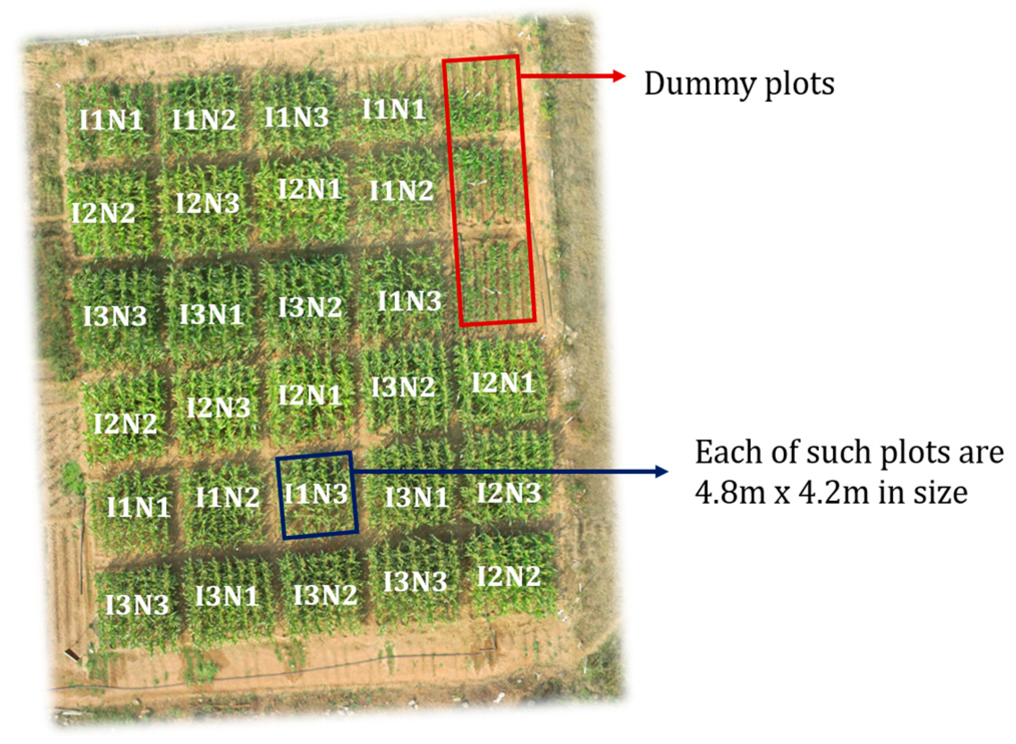
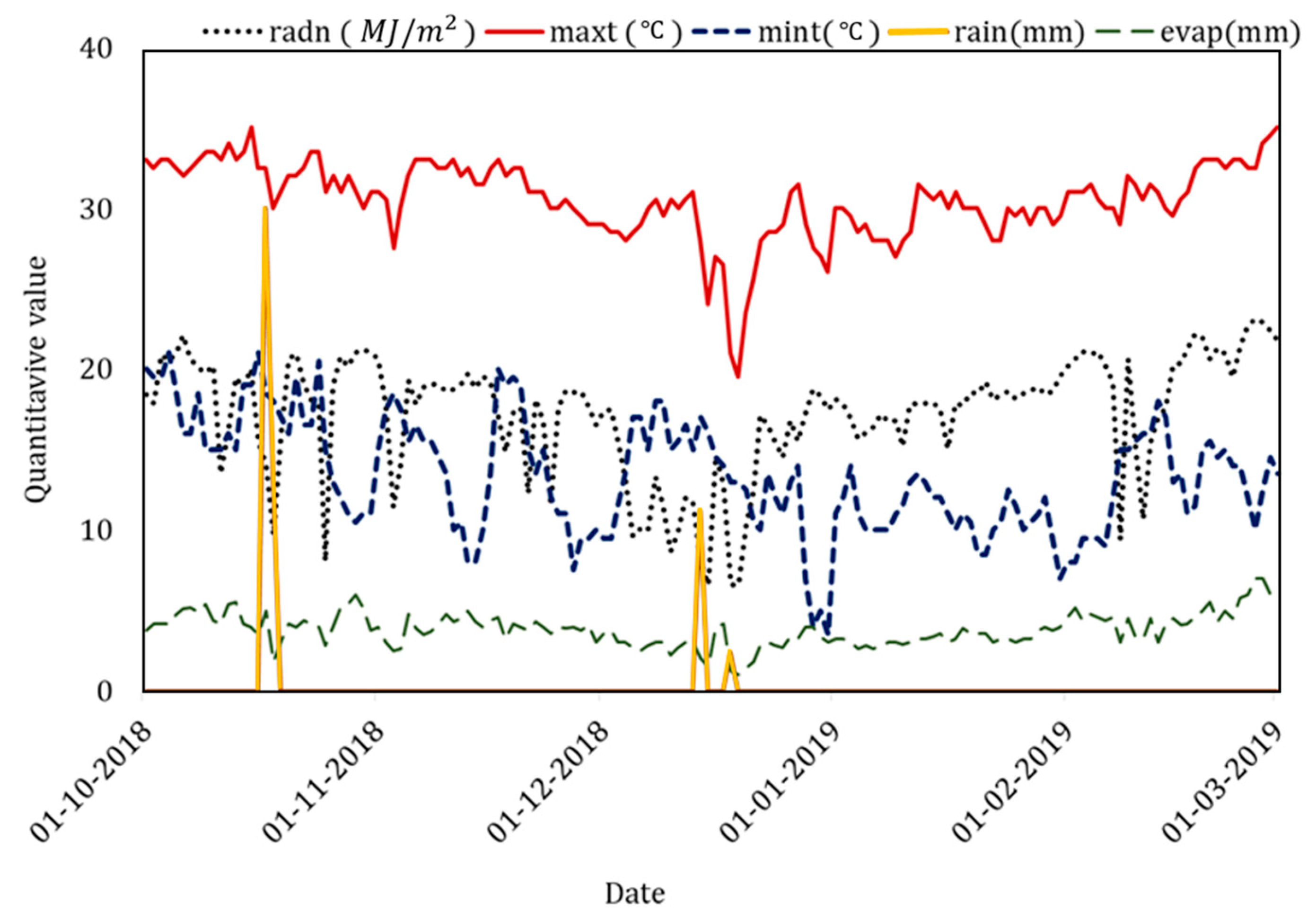
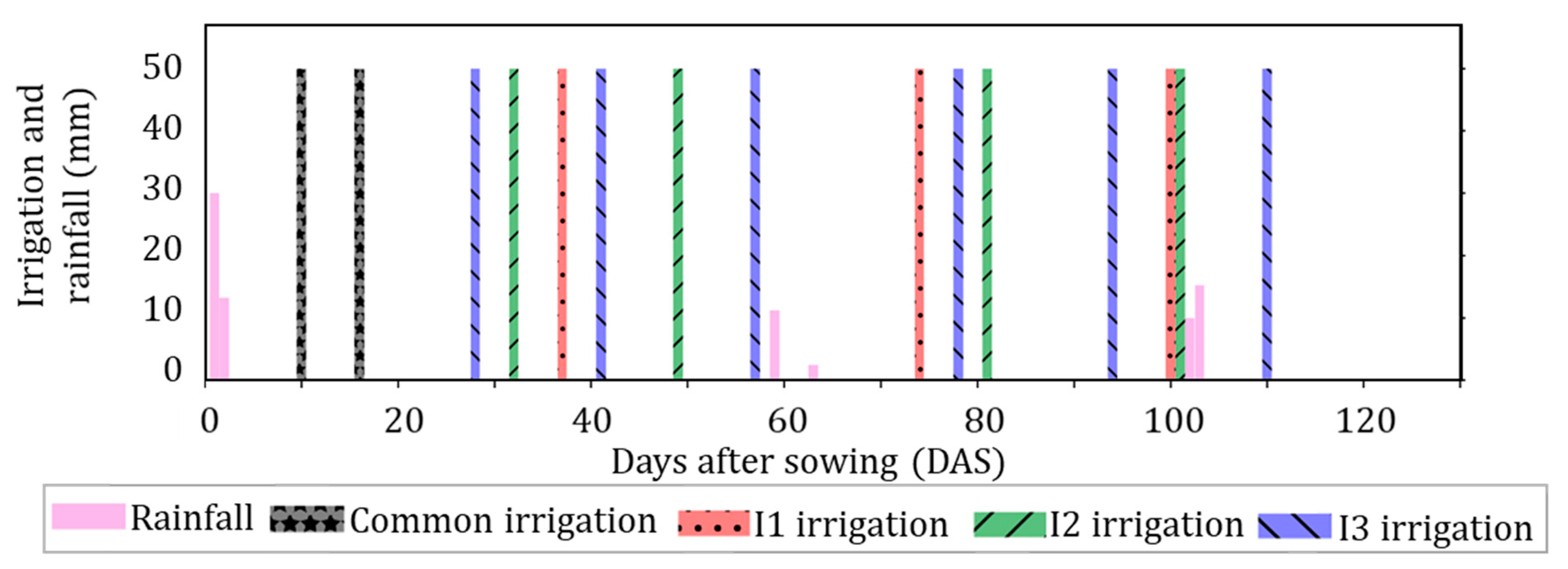
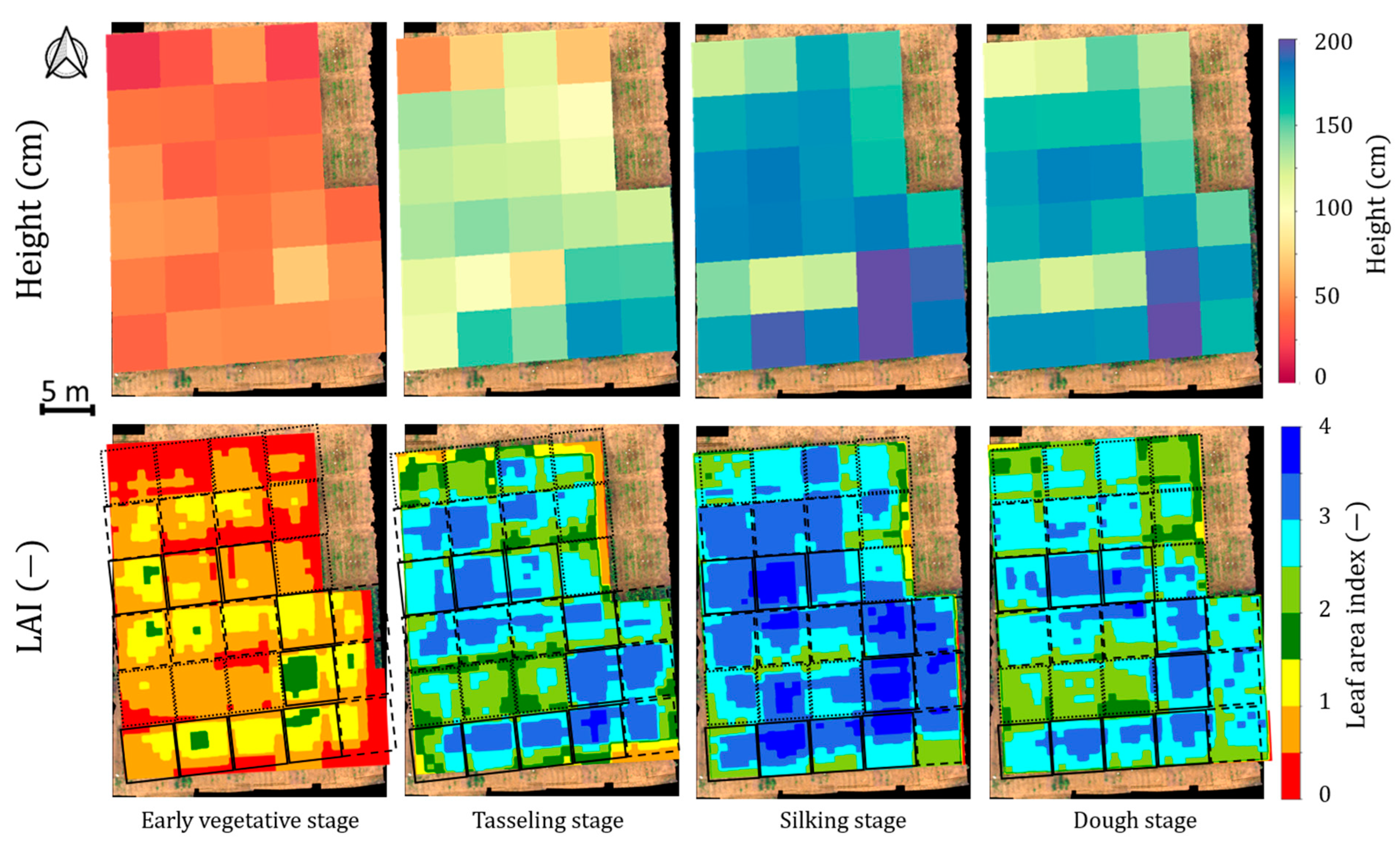
This research has used the data presented by Raj et al., 2021 [29]. The dataset was collected in 2018–2019 from a maize (variety: Cargil 900 M gold) research farm developed in the semi-arid region of Hyderabad district of India (7°19′27.2″ N, 78°23′55.4″ E). A total of 27 maize plots, each having an area of 4.2 m × 4.8 m, were treated with a combination of three different water and nitrogen levels to grow the crop under nine different management variable conditions. The nine unique treatments were replicated thrice, with the plot setting as shown in Figure 2. The text written above each plot in Figure 2 indicates the irrigation and nitrogen treatments applied to the corresponding plots. Here, ‘I’ stands for irrigation and ‘N’ stands for nitrogen. The numbers written after these letters (e.g., 1, 2, or 3) indicate the level of irrigation and fertilization, respectively, where ‘1’ denotes a low amount of supply and ‘3’ is used for a high amount of supply. The detailed management practices were discussed in Raj et al., 2021 [29]. All the plots had a sandy loam soil type, 8.33 plants per square meter crop density, same weather conditions (shown in Figure 3), and furrow irrigation. A summary of the data is shown in Table 1, with the details of the data available in the papers mentioned above. Weather data, soil property information, and management practice details used for simulation of the APSIM model are shown in Figure 3, Table 2, and Figure 4, respectively. The crop height and LAI map were generated according to Raj et al., 2021, [29] and used as inputs in the crop healthiness map model. The height map was generated for each plot, while the LAI map was created for each square meter. Figure 5 shows the generated LAI and height map. The pixel size for the height map is equal to the plot size, and spatial resolution of the LAI map was taken as one meter.

2.2. APSIM Model

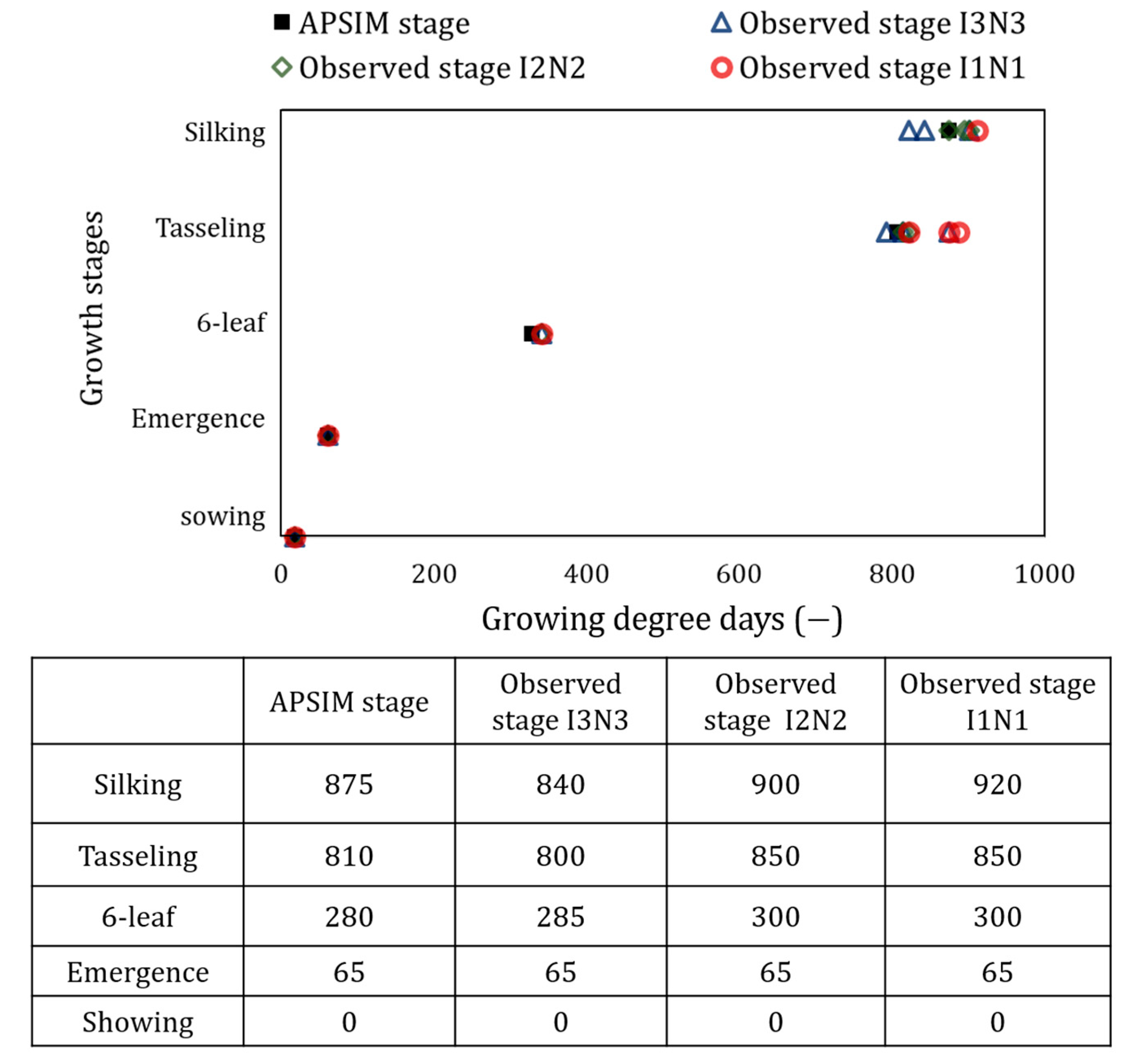
The APSIM (Agricultural Production Systems sIMulator [30]) model was used to simulate crop growth under actual farm weather and applied irrigation/fertilization conditions with identified soil properties. Temporal values of crop LAI, canopy height, and soil moisture of all the plots were simulated and used as a reference to compare with actual farm data. The maize seed variety used for farming was ‘Cargil 900 m gold’; however, this maize seed variety was not available in APSIM. Accordingly, the seed variety was selected from available APSIM options based on a comparative analysis of growing degree days (GDD) and the onset of growth stages with respect to farm-observed responses. The simulation of the model with different seed varieties led to selection of the ‘mh12′ seed type, as it mimics the same behaviour as the ‘Cargil 900 m gold’. Figure 6 shows the field observed growth stage occurrence with respect to change in GDD for APSIM simulation of the ‘mh12′ maize variety. The soil and weather properties were taken as per recorded farm conditions. The values below the graph of Figure 6 show the average GDD value for the three replicated plots for each treatment. The GDD difference between simulated and observed growth stages was less than 100 for the tasseling and silking stages, while the differences were negligible for the emergence and 6-leaf stage. The similarity between the simulated and observed growth stage values was considered as the indicator of the acceptability of the APSIM model results, without requiring intensive calibration of the model using field data.
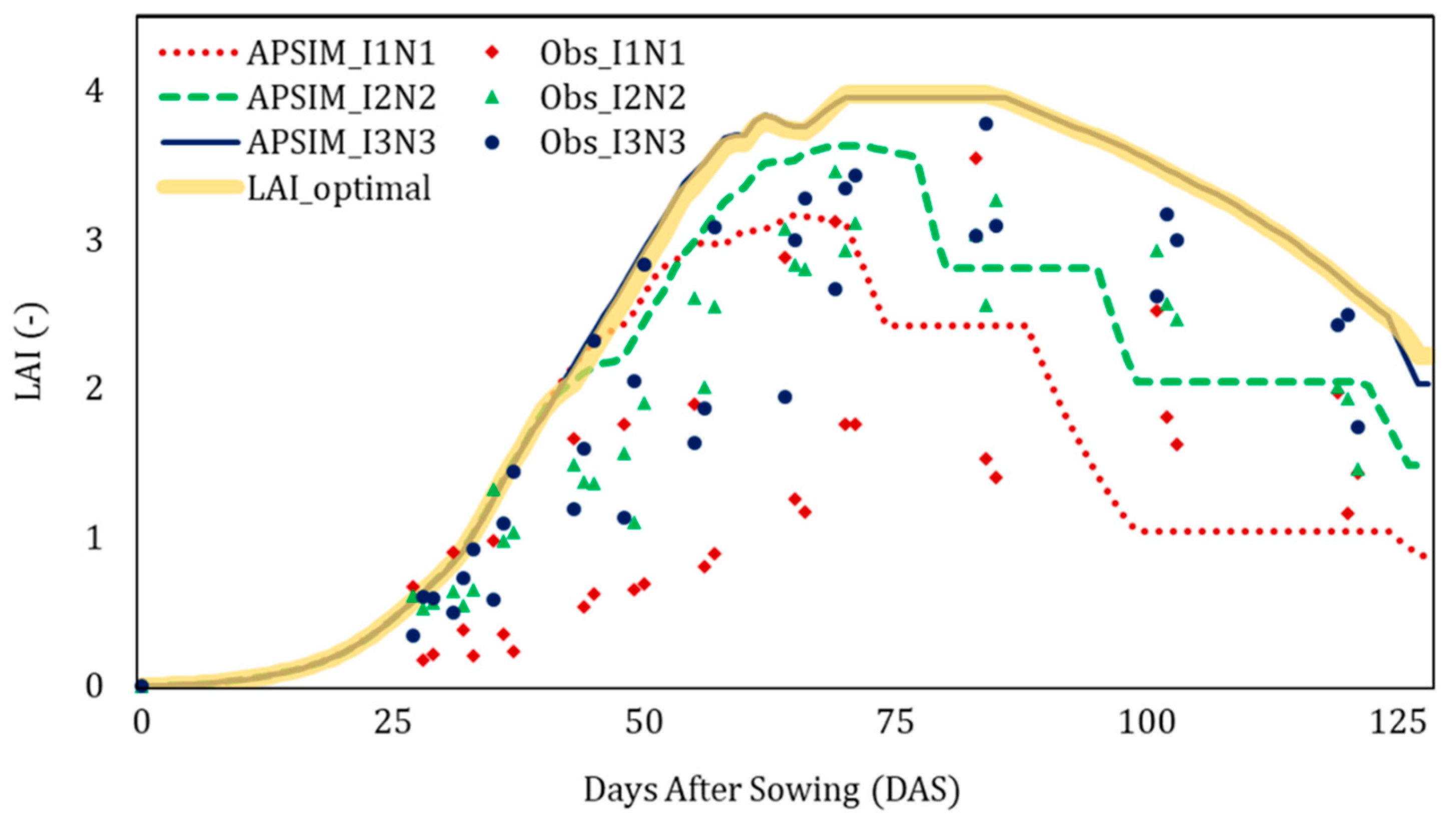
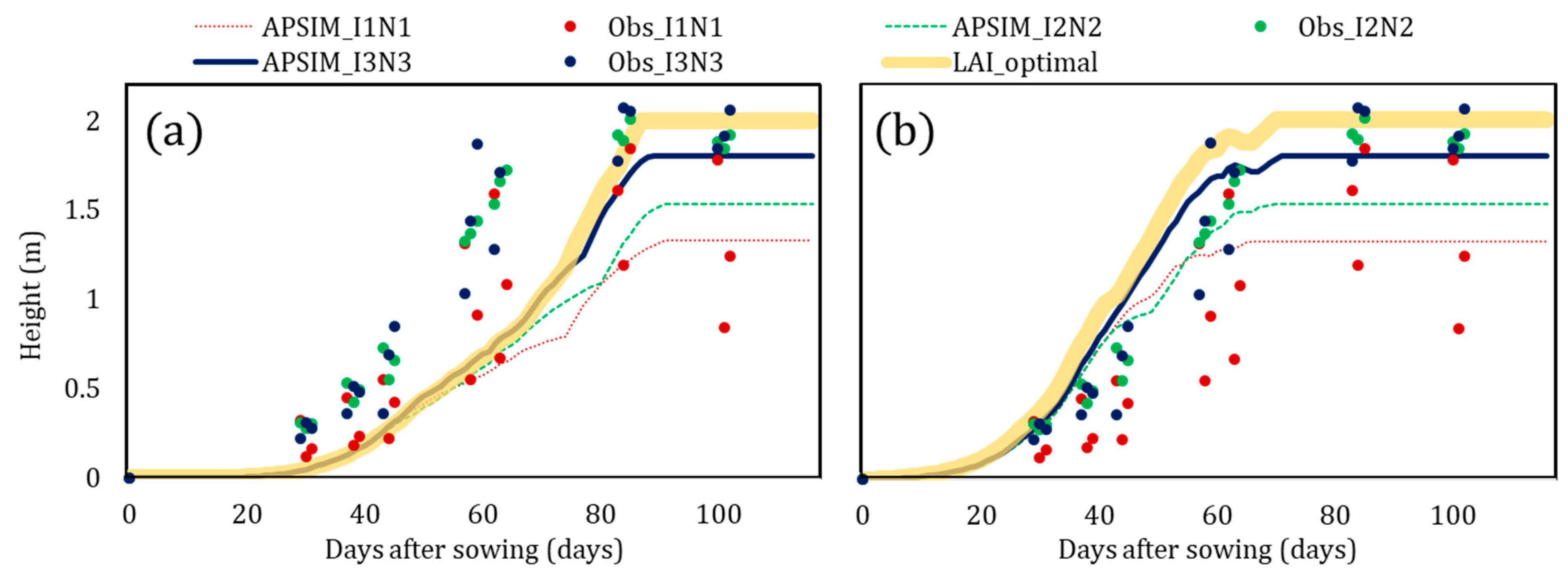
The LAI and canopy height of maize were simulated in APSIM, and simulated output were compared against the observed LAI and height values of respective treatment plots. It was found that the APSIM model simulation of LAI and height was insensitive to changes in water and nutrients during the initial growth stage, but had greater sensitivity as it progressed towards the maturity stage. Figure 7 shows the simulated and observed canopy LAI values, with the simulated initial growth stage LAI being always equal to the optimal condition simulation of LAI. The model seems to be insensitive during the initial growth stage and remains at optimal values even for low irrigation and low fertilization treatment plots. The optimal values were simulated by maintaining the simulated soil moisture above 70% of the field capacity. Moreover, the simulated canopy height was underestimated compared to the observed farm values for all scenarios, as shown in Figure 8a. The problem of canopy height underestimation was resolved by updating the height values proportional to the rate of change of simulated LAI until the canopy closure stage. This was conducted in consideration of a high correlation between canopy height and LAI [31]. The updated canopy height graph is shown in Figure 8b.
The graphs show that the APSIM-simulated result for early crop growth stages is not sensitive to management practices without proper calibration. However, the optimal condition simulated values can be used as a reference. Moreover, the simulated values for late growth stages were close to the field observed values, making the APSIM model results useful. These optimal values were therefore used to create synthetic data to build linear and random forest models. In comparison to the random forest model, the linear model is less demanding in terms of computational resources and data, making it suitable for use on low compute-intensive machines with slight compromise on the model accuracy.

2.3. Linear Model for Crop Healthiness

In the linear approach, LAI and height maps were used to predict the crop stress level using a Healthiness Index, which should be taken as an indicator to identify the crop healthiness based on its biophysical parameters (LAI and height). The areas having low Healthiness Index indicate a high chance of the crop being stressed. Two thresholds have been created to determine the stress levels in the crop, with the crop considered healthy if the drone-based LAI and height values are around the APSIM-simulated optimal values. However, the plots were considered severely stressed if the observed values were equal to or less than 0.55 and 0.65 times the simulated optimal LAI and height, respectively. The stress condition thresholds were calculated by averaging simulation values of the I1N1 condition post canopy closure. All observations in between optimal and stressed levels were linearly scaled, with the thresholds given in Table 3. The formula used to predict the healthiness/stress level using the Healthiness Index of the plots is given as
H e a l t h i n e s s   I n d e x = L A I p r e d + H e i g h t p r e d 2 ,
where
L A I p r e d = 2 × L A I o b s e r v e d L A I o p t i m a l 1 ,
H e i g h t p r e d = 2.5 × H e i g h t o b s e r v e d H e i g h t o p t i m a l 1.5 ,
such that L A I o b s e r v e d and H e i g h t o b s e r v e d are the remotely sensed values of LAI and height of the crop, respectively. L A I o p t i m a l and H e i g h t o p t i m a l are the APSIM-simulated optimal values for LAI and height, respectively, for the corresponding crop age (days after sowing—DAS).
The Healthiness Index is a value between 0 and 1, where stressed plants are indicated by 0 and healthy plants by 1. This linear model was implemented on the drone-based LAI and height. If the RGB image-based LAI or height (observed) values were greater than the simulated optimal value or less than the severe stress condition value (as shown in Table 3), then the observed value was made equal to the nearest threshold, i.e., either simulated optimal value or severe stress condition value.

2.4. Random Forest Model for Crop Healthiness

The Random Forest (RF) model has emerged as a highly influential and effective ensemble learning method in the field of predictive analysis [32]. By combining the principles of decision trees and the concept of ensemble learning, RF has garnered significant attention and acclaim due to its exceptional performance in diverse domains including agriculture [33]. Selection of the RF machine learning model was made considering its proven ability to be less sensitive towards the quality of training samples and overfitting [34]. Accordingly, the RF approach used two inputs—LAI and crop height—to predict the crop healthiness level. The training data for the RF model were synthetically generated using reference values from APSIM-simulated values.
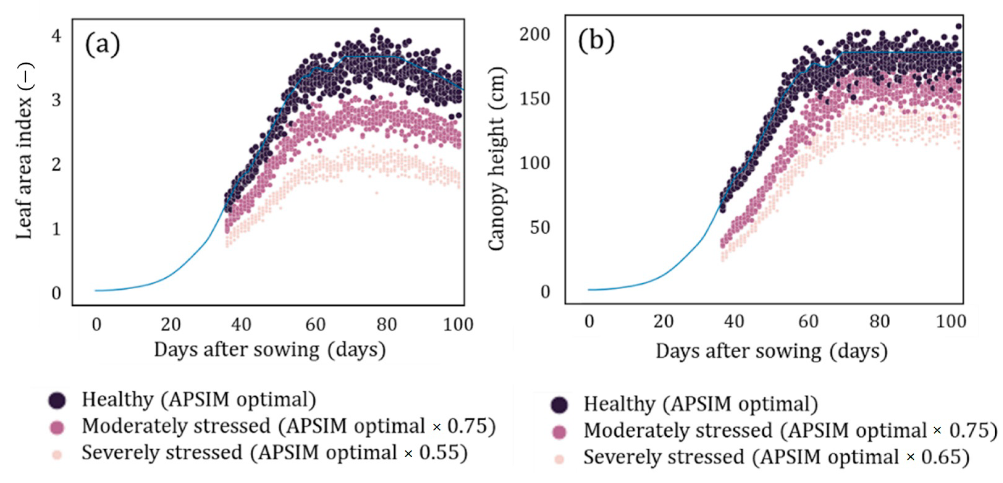
The process of creating synthetic data was as follows. If the observed (drone-based) LAI and height values are close to APSIM-simulated optimal values, it was considered a healthy crop condition. However, the plots were considered severely stressed if the observed values were equal to or less than 0.55 and 0.65 times the simulated optimal LAI and height, respectively (same as in the linear model). Moderate stress condition was considered when observed values were around 0.75 times the simulated optimal LAI and canopy height. These scaled values were used as the mean, and with a 5% standard deviation around each of these values, random gaussian noise was generated. A total of 1000 sample values were generated for each condition. The generated synthetic data are shown in Figure 9.
The RF model was trained on the synthetic data, with the hyperparameter values tuned to obtain the best-suited values. The created RF model had n_estimators = 1400, random_state = 42, criterion = entropy, and min_samples_split = 10. The model output ranged from 0 to 1, indicating 0 for stressed plots and 1 for healthy plots. These values were named Healthiness Index. This model was then implemented on the drone-based LAI, and crop height maps and Healthiness Index farm maps obtained.

3. Results and Discussion

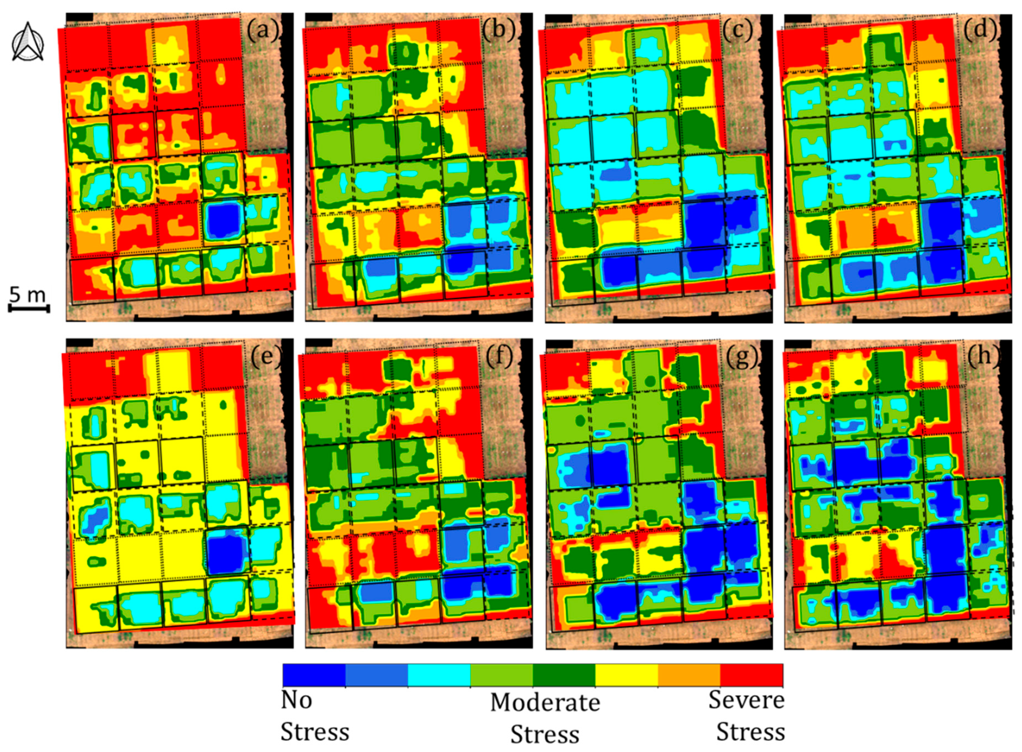
Crop healthiness maps for different growth stages were made using the linear and RF model. Figure 10 shows the results of the linear and RF models on temporal drone data. The four growth stages considered for analysis were the early vegetative stage, tasseling stage, silking stage, and dough stage. Figure 10a–d displays the results of the linear model, while 10e–h present the results of the RF model. In Figure 10a,e, which represent the early vegetative stage stress maps, the linear model (Figure 10a) classifies most of the moderately stressed plots as severe stress (red color). However, the RF model assigns these plots closer to the moderate stress class, although not precisely matching the actual conditions. The disparity in stress maps can be attributed to the crop’s shorter height and LAI in the early vegetative stage, resulting in a higher error percentage compared to later growth stages. Figure 10b–c and 10f–g show the tasseling- and silking-stage crop stress maps for the linear and RF models, respectively. The accuracy of the tasseling-stage model exhibits similar results, but the linear model’s silking-stage results classify some plots closer to the no stress condition, which is not consistent with actual farm observations. Figure 10d,h represents the dough-stage farm stress map, showing the highest correlation with crop yield. However, at the dough stage, the RF model produces stress map results that are closer to the ground observations.
The Random Forest result was found to be more accurate, being able to differentiate between I3, I2, and I1 plots more efficiently. The model’s performance improved as the crop moved towards the maturity stage, with the dough-stage healthiness map making all I3, I2, and I1 plots distinguishable from other stage crops.
Quantitative analysis of the models was undertaken by correlating the plot-wise average values of the predicted healthiness level (between 0–1) with the yield values. Figure 11 shows the scatter plot correlation values for the 6-leaf, tasseling, silking, and dough stages. It was found that the RF model performed relatively better than the linear model for all growth stages. For the early vegetative stage (6-leaf stage), the obtained R2 was 0.42 and 0.45 for the linear and RF model, respectively. For the tasseling stage, R2 for the linear model was 0.56, and for the RF model, it was 0.61. The silking stage results were similar to the tasseling stage, with R2 of 0.56 and 0.58 for the linear and RF models, respectively. The dough stage gave the best performance, with R2 of 0.63 and 0.67 for the linear and RF models, respectively. In general, as the growth stage progress, R2 values appeared to be increasing for both the models, but the RF model performance was found to be better than the linear model.
The relationship between crop healthiness and crop yield was expected to strengthen as the growth stage advanced. This finding aligns with previous research conducted on a larger scale using MODIS data [35], which utilized vegetation indices to estimate maize yield. In that study, the highest correlation coefficient achieved was 0.67, observed as the crop transitioned from the vegetative stage to maturity. Similarly, in a separate investigation, researchers employed drone-based RGB images to estimate sugarcane yield based on LAI and the Green-Red vegetation Index [36], obtaining R2 values ranging from 0.69 to 0.79. These results were obtained around the inflection point of the biomass accumulation curve, typically occurring a few days prior to crop maturity. The healthiness level during the initial growth stage may impact the end-of-season crop yield, but the management practices during the intermediate stages can influence the yield, which may not be reflected when using only initial growth stage data. Figure 10 maps demonstrate how plots initially experiencing severe stress could improve their healthiness over time, eventually being classified as under moderate stress conditions by the silking or dough stage. When the crop is closer to maturity, there is an expected higher correlation between healthiness level and crop yield as the input data to the model represents the cumulative effect of management practices on the crop.
The parameters of this model were specifically designed for the maize crop, with the variety being Cargil 900 M gold, and they are expected to work better with the same variety. To replicate the model for other crops or varieties, a similar methodology should be adopted to create crop-specific models. When interpreting the results, it is important to consider that the research plots, as shown in Figure 2, were treated with varying irrigation and fertilization techniques while being in close proximity to each other. Although precautions were taken to physically separate the plots and prevent surface transfer of irrigation water among them, it is still possible for water to seep underground and potentially affect neighboring plots, particularly due to its sandy-loam nature. Such occurrences have the potential to impact the treatment effects on the crop.
Temporal crop healthiness mapping plays a crucial role in determining the overall productivity of agricultural crops. The connection between crop health and yield stems from the fact that healthy plants are more likely to exhibit optimal growth, resist pests and diseases, and efficiently utilize available resources. By monitoring the temporal patterns of crop health indicators, the agricultural community can assess the vitality and vigor of their crops over time. Timely identification of any deviations from the expected health trajectory allows for prompt interventions, including adjusting nutrient levels, water supply, or implementing appropriate pest management strategies. By maintaining optimal crop health throughout the growing season, farmers can maximize the potential yield of their crops and ensure the economic viability and sustainability of their agricultural operations.
The findings of this research highlight a clear relationship between the severity of crop stress and reductions in crop biophysical parameters such as LAI and height. These observations are consistent with the existing literature on crop processes [37,38]. As the severity of stress increases, the reduction from optimal values becomes more pronounced. This reduction becomes particularly noticeable as the crop progresses beyond the vegetative stage. For crops subjected to one-third of the recommended irrigation, the yield was reduced by approximately threefold, with observed crop LAI and height reaching only 55% and 70% of their optimal values, respectively. Similar observations have been reported by other researchers [39,40].
Exploring the published research on similar topics reveals noteworthy findings. In one study [41], UAV-based multispectral data were utilized to estimate LAI, which was further assimilated with ground monitoring data to estimate crop yield, resulting in an R2 value of 0.85. Another study [42] found that the use of surface temperature and vegetation index derived from MODIS data for estimating crop yield varied based on agroclimatic zones, yielding R2 values between 0.68 and 0.81 for crops such as wheat and soybean. For potato crop yield prediction using Sentinel-2 multispectral data, a maximum R2 of 0.65 was obtained in a separate study [43]. Similarly, in a very similar study, researchers used MODIS-derived vegetation indices to estimate corn crop yield during the harvesting stage, achieving a maximum R2 value of 0.72 [44]. Interestingly, the literature shows that most researchers have used multispectral data for determining crop stress. However, the presented research has demonstrated the capability of RGB images to estimate crop stress.

4. Conclusions

This study concludes that remotely estimated crop biophysical parameters from RGB images-based observations, such as LAI and height, can be used as a low-cost (compared to multispectral and hyperspectral sensors) but no less effective solution for identifying stressed and healthy areas on the maize farm. However, the healthiness maps developed in this research cannot indicate the reason for the stress, which would require an onsite inspection. The performance of the developed models was found to improve as the crop matured, with the dough stage producing the best results. The study’s findings provide valuable insights into the impact of stress on crop health, which can aid in developing strategies to mitigate its effects, ultimately improving crop yield and food security by enabling farmers to make data-driven decisions and implement targeted interventions in near real-time, resulting in efficient resource management and higher crop yields. The use of biophysical properties derived from low-cost airborne RGB images has therefore been shown to have promise in identifying stressed areas on farms. However, the accuracy and precision of these biophysical properties can be influenced by several factors, and more research is needed to develop and test methods such as machine learning algorithms that can automatically identify stressed areas and to integrate different data sources to improve the accuracy and precision of crop stressed area identification on farms. The development and use of these technologies will have important implications for the development of sustainable agriculture practices and the optimization of crop yields.

Author Contributions

R.R.—Conceptualization, methodology, software, validation, formal analysis, data curation, writing original draft preparation; J.P.W.—Conceptualization, investigation, resources, writing, review, supervision; A.J.—Investigation, resources, review and editing, supervision, project administration, funding acquisition. All authors have read and agreed to the published version of the manuscript.

Funding

This research was jointly funded by the Department of Science and Technology (DST); Ministry of Science and Technology, Government of India; and Japan Science and Technology (JST), Government of Japan (DST/INT/JST/P-29/2016) between years 2016–2021.

Institutional review board statement

Not applicable.

Data Availability Statement

Data will be made available on request.

Acknowledgments

The authors would like to thank Rohit Nandan, Balaji, Rohit Pingale, and Dishank Jindal for their technical discussions and resource support during the research.

Conflicts of Interest

The authors declare no conflict of interest.

References

  1. Glendining, M.J.; Dailey, A.G.; Williams, A.G.; Van Evert, F.K.; Goulding, K.W.T.; Whitmore, A.P. Is it possible to increase the sustainability of arable and ruminant agriculture by reducing inputs? Agric. Syst. 2009, 99, 117–125. [Google Scholar] [CrossRef] [Green Version]
  2. Maraveas, C.; Piromalis, D.; Arvanitis, K.G.; Bartzanas, T.; Loukatos, D. Applications of IoT for optimized greenhouse environment and resources management. Comput. Electron. Agric. 2022, 198, 106993. [Google Scholar] [CrossRef]
  3. Ragavi, V.; Subburaj, J.; Keerthana, P.; Soundaryaveni, C. Smart Agriculture to increase Farmers Profitability using Internet of Things. Indian J. Sci. Technol. 2019, 12, 1–6. [Google Scholar] [CrossRef]
  4. Daponte, P.; De Vito, L.; Glielmo, L.; Iannelli, L.; Liuzza, D.; Picariello, F.; Silano, G. A Review on the Use of Drones for Precision Agriculture; IOP Conference Series: Earth and Environmental Science; IOP Publishing: Bristol, UK, 2019; Volume 275, p. 012022. [Google Scholar]
  5. Adrian, A.M.; Norwood, S.H.; Mask, P.L. Producers’ perceptions and attitudes toward precision agriculture technologies. Comput. Electron. Agric. 2005, 48, 256–271. [Google Scholar] [CrossRef]
  6. Broge, N.H.; Mortensen, J.V. Deriving green crop area index and canopy chlorophyll density of winter wheat from spectral reflectance data. Remote Sens. Environ. 2002, 81, 45–57. [Google Scholar] [CrossRef]
  7. Radočaj, D.; Šiljeg, A.; Marinović, R.; Jurišić, M. State of Major Vegetation Indices in Precision Agriculture Studies Indexed in Web of Science: A Review. Agriculture 2023, 13, 707. [Google Scholar] [CrossRef]
  8. Sun, H. Crop Vegetation Indices. In Encyclopedia of Smart Agriculture Technologies; Springer International Publishing: Cham, Switzerland, 2023; pp. 1–7. [Google Scholar]
  9. Mwinuka, P.R.; Mourice, S.K.; Mbungu, W.B.; Mbilinyi, B.P.; Tumbo, S.D.; Schmitter, P. UAV-based multispectral vegetation indices for assessing the interactive effects of water and nitrogen in irrigated horticultural crops production under tropical sub-humid conditions: A case of African eggplant. Agric. Water Manag. 2022, 266, 107516. [Google Scholar] [CrossRef]
  10. Ihuoma, S.O.; Madramootoo, C.A. Sensitivity of spectral vegetation indices for monitoring water stress in tomato plants. Comput. Electron. Agric. 2019, 163, 104860. [Google Scholar] [CrossRef]
  11. Zhang, L.; Han, W.; Niu, Y.; Chávez, J.L.; Shao, G.; Zhang, H. Evaluating the sensitivity of water stressed maize chlorophyll and structure based on UAV derived vegetation indices. Comput. Electron. Agric. 2021, 185, 106174. [Google Scholar] [CrossRef]
  12. Townshend, J.R.; Goff, T.E.; Tucker, C.J. Multitemporal dimensionality of images of normalized difference vegetation index at continental scales. IEEE Trans. Geosci. Remote Sens. 1985, 6, 888–895. [Google Scholar] [CrossRef]
  13. Becker, F.; Choudhury, B.J. Relative sensitivity of normalized difference vegetation Index (NDVI) and microwave polarization difference Index (MPDI) for vegetation and desertification monitoring. Remote Sens. Environ. 1988, 24, 297–311. [Google Scholar] [CrossRef]
  14. Pettorelli, N. The normalized difference vegetation index; Oxford University Press: Hong Kong, China, 2013. [Google Scholar]
  15. Suárez, L.; Zarco-Tejada, P.J.; Sepulcre-Cantó, G.; Pérez-Priego, O.; Miller, J.R.; Jiménez-Muñoz, J.C.; Sobrino, J. Assessing canopy PRI for water stress detection with diurnal airborne imagery. Remote Sens. Environ. 2008, 112, 560–575. [Google Scholar] [CrossRef]
  16. Han, M.; Zhang, H.; DeJonge, K.C.; Comas, L.H.; Trout, T.J. Estimating maize water stress by standard deviation of canopy temperature in thermal imagery. Agric. Water Manag. 2016, 177, 400–409. [Google Scholar] [CrossRef]
  17. Anjum, S.A.; Ashraf, U.; Zohaib, A.; Tanveer, M.; Naeem, M.; Ali, I.; Tabassum, T.; Nazir, U. Growth and development responses of crop plants under drought stress: A review. Zemdirbyste 2017, 104, 267–276. [Google Scholar] [CrossRef]
  18. Baret, F.; Houles, V.; Guerif, M. Quantification of plant stress using remote sensing observations and crop models: The case of nitrogen management. J. Exp. Bot. 2007, 58, 869–880. [Google Scholar] [CrossRef] [PubMed] [Green Version]
  19. Wittstruck, L.; Jarmer, T.; Trautz, D.; Waske, B. Estimating LAI From Winter Wheat Using UAV Data and CNNs. IEEE Geosci. Remote Sens. Lett. 2022, 19, 3141497. [Google Scholar] [CrossRef]
  20. Yucky, E.D.D.; Putrada, A.G.; Abdurohman, M. IoT drone camera for a paddy crop health detector with RGB comparison. In Proceedings of the 2021 9th International Conference on Information and Communication Technology (ICoICT), Yogyakarta, Indonesia, 3–5 August 2021; IEEE: Piscataway, NJ, USA; pp. 155–159. [Google Scholar]
  21. Garza, B.N.; Ancona, V.; Enciso, J.; Perotto-Baldivieso, H.L.; Kunta, M.; Simpson, C. Quantifying Citrus Tree Health Using True Color UAV Images. Remote Sens. 2020, 12, 170. [Google Scholar] [CrossRef] [Green Version]
  22. Candiago, S.; Remondino, F.; De Giglio, M.; Dubbini, M.; Gattelli, M. Evaluating Multispectral Images and Vegetation Indices for Precision Farming Applications from UAV Images. Remote Sens. 2015, 7, 4026–4047. [Google Scholar] [CrossRef] [Green Version]
  23. Catania, P.; Roma, E.; Orlando, S.; Vallone, M. Evaluation of Multispectral Data Acquired from UAV Platform in Olive Orchard. Horticulturae 2023, 9, 133. [Google Scholar] [CrossRef]
  24. Franke, J.; Menz, G. Multi-temporal wheat disease detection by multi-spectral remote sensing. Precis. Agric. 2007, 8, 161–172. [Google Scholar] [CrossRef]
  25. Shafi, U.; Mumtaz, R.; Iqbal, N.; Zaidi, S.M.H.; Zaidi, S.A.R.; Hussain, I.; Mahmood, Z. A Multi-Modal Approach for Crop Health Mapping Using Low Altitude Remote Sensing, Internet of Things (IoT) and Machine Learning. IEEE Access 2020, 8, 112708–112724. [Google Scholar] [CrossRef]
  26. Khan, A.; Vibhute, A.D.; Mali, S.; Patil, C. A systematic review on hyperspectral imaging technology with a machine and deep learning methodology for agricultural applications. Ecol. Informatics 2022, 69, 101678. [Google Scholar] [CrossRef]
  27. Krishna, G.; Sahoo, R.N.; Singh, P.; Patra, H.; Bajpai, V.; Das, B.; Kumar, S.; Dhandapani, R.; Vishwakarma, C.; Pal, M.; et al. Application of thermal imaging and hyperspectral remote sensing for crop water deficit stress monitoring. Geocarto Int. 2021, 36, 481–498. [Google Scholar] [CrossRef]
  28. Vasavi, P.; Punitha, A.; Rao, T.V.N. Crop leaf disease detection and classification using machine learning and deep learning algorithms by visual symptoms: A review. Int. J. Electr. Comput. Eng. 2022, 12, 2079–2086. [Google Scholar] [CrossRef]
  29. Raj, R.; Walker, J.P.; Pingale, R.; Nandan, R.; Naik, B.; Jagarlapudi, A. Leaf area index estimation using top-of-canopy airborne RGB images. Int. J. Appl. Earth Obs. Geoinf. 2021, 96, 102282. [Google Scholar] [CrossRef]
  30. Keating, B.A.; Carberry, P.S.; Hammer, G.L.; Probert, M.E.; Robertson, M.J.; Holzworth, D.; Huth, N.I.; Hargreaves, J.N.; Meinke, H.; Hochman, Z.; et al. An overview of APSIM, a model designed for farming systems simulation. Eur. J. Agron. 2003, 18, 267–288. [Google Scholar] [CrossRef] [Green Version]
  31. Luo, S.; Wang, C.; Xi, X.; Nie, S.; Fan, X.; Chen, H.; Yang, X.; Peng, D.; Lin, Y.; Zhou, G. Combining hyperspectral imagery and LiDAR pseudo-waveform for predicting crop LAI, canopy height and above-ground biomass. Ecol. Indic. 2019, 102, 801–812. [Google Scholar] [CrossRef]
  32. Breiman, L. Random forests. Mach. Learn. 2001, 45, 5–32. [Google Scholar] [CrossRef] [Green Version]
  33. Guo, Y.; Chen, S.; Li, X.; Cunha, M.; Jayavelu, S.; Cammarano, D.; Fu, Y. Machine Learning-Based Approaches for Predicting SPAD Values of Maize Using Multi-Spectral Images. Remote Sens. 2022, 14, 1337. [Google Scholar] [CrossRef]
  34. Belgiu, M.; Drăguţ, L. Random forest in remote sensing: A review of applications and future directions. ISPRS J. Photogramm. Remote Sens. 2016, 114, 24–31. [Google Scholar] [CrossRef]
  35. Bolton, D.K.; Friedl, M.A. Forecasting crop yield using remotely sensed vegetation indices and crop phenology metrics. Agric. For. Meteorol. 2013, 173, 74–84. [Google Scholar] [CrossRef]
  36. Sanches, G.M.; Duft, D.G.; Kölln, O.T.; Luciano, A.C.D.S.; De Castro, S.G.Q.; Okuno, F.M.; Franco, H.C.J. The potential for RGB images obtained using unmanned aerial vehicle to assess and predict yield in sugarcane fields. Int. J. Remote Sens. 2018, 39, 5402–5414. [Google Scholar] [CrossRef]
  37. Nielsen, D.C.; Halvorson, A.D. Nitrogen Fertility Influence on Water Stress and Yield of Winter Wheat. Agron. J. 1991, 83, 1065–1070. [Google Scholar] [CrossRef] [Green Version]
  38. Wilhelm, W.W.; Ruwe, K.; Schlemmer, M.R. Comparison of Three Leaf Area Index Meters in a Corn Canopy. Crop Sci. 2000, 40, 1179–1183. [Google Scholar] [CrossRef]
  39. Gano, B.; Dembele, J.S.B.; Ndour, A.; Luquet, D.; Beurier, G.; Diouf, D.; Audebert, A. Using UAV Borne, Multi-Spectral Imaging for the Field Phenotyping of Shoot Biomass, Leaf Area Index and Height of West African Sorghum Varieties under Two Contrasted Water Conditions. Agronomy 2021, 11, 850. [Google Scholar] [CrossRef]
  40. Zhang, L.; Niu, Y.; Zhang, H.; Han, W.; Li, G.; Tang, J.; Peng, X. Maize Canopy Temperature Extracted From UAV Thermal and RGB Imagery and Its Application in Water Stress Monitoring. Front. Plant Sci. 2019, 10, 1270. [Google Scholar] [CrossRef]
  41. Peng, X.; Han, W.; Ao, J.; Wang, Y. Assimilation of LAI Derived from UAV Multispectral Data into the SAFY Model to Estimate Maize Yield. Remote Sens. 2021, 13, 1094. [Google Scholar] [CrossRef]
  42. Holzman, M.E.; Rivas, R.; Piccolo, M.C. Estimating soil moisture and the relationship with crop yield using surface temperature and vegetation index. Int. J. Appl. Earth Obs. Geoinformation 2014, 28, 181–192. [Google Scholar] [CrossRef]
  43. Al-Gaadi, K.A.; Hassaballa, A.A.; Tola, E.; Kayad, A.G.; Madugundu, R.; Alblewi, B.; Assiri, F. Prediction of Potato Crop Yield Using Precision Agriculture Techniques. PLoS ONE 2016, 11, e0162219. [Google Scholar] [CrossRef] [Green Version]
  44. Ji, Z.; Pan, Y.; Zhu, X.; Wang, J.; Li, Q. Prediction of Crop Yield Using Phenological Information Extracted from Remote Sensing Vegetation Index. Sensors 2021, 21, 1406. [Google Scholar] [CrossRef]
Figure 1. Framework for identifying crop stress areas using drone-based LAI and canopy height maps.
Agriculture 13 01292 g001
Figure 2. A top-of-canopy view of each plot of the research farm. The text over the plots indicate the irrigation (I) and nitrogen (N) treatments given to the plots.
Agriculture 13 01292 g002
Figure 3. The weather data used for simulation of the APSIM model, where ‘radn’ is solar radiation, ‘maxt’ is daily maximum temperature, ‘mint’ is daily minimum temperature, ‘rain’ is daily rainfall, and ‘evap’ is daily evaporation values.
Agriculture 13 01292 g003
Figure 4. Irrigation timing information for plots at different water stress conditions. Fertilization was given to plots just before irrigation to respective plots.
Agriculture 13 01292 g004
Figure 5. Temporal height and LAI maps of maize farm created using model adopted from Raj et al. (2021) [29]. Solid line boxes represent sufficiently irrigated plots, dashed line boxes for moderately irrigated, and less irrigated plots are shown with dotted line boxes.
Agriculture 13 01292 g005
Figure 6. Growing degree days (GDD)-based growth stage occurrence from APSIM simulations and observed farm data for the ‘mh12′ seed variety. Ix and Nx represent irrigation and nitrogen status, where x having the number 1 denotes low, 2 denotes moderate, and 3 denotes high conditions.
Agriculture 13 01292 g006
Figure 7. Simulated (APSIM) and observed (Obs) temporal LAI of different treatment plots.
Agriculture 13 01292 g007
Figure 8. (a) Simulated and observed temporal canopy height for different treatment plots, with the model highly underestimating the canopy height until the tasseling/silking (canopy closure) stage. (b) Canopy height output after updating the height values proportional to the rate of change of LAI until the canopy closure stage.
Agriculture 13 01292 g008
Figure 9. Synthetic data plot for (a) LAI and (b) canopy height, showing three levels of crop healthiness. The reference for these thresholds was taken from APSIM-simulated results for the I1N1, I2N2, and optimal condition plots. The light blue line indicates APSIM-simulated optimal value.
Agriculture 13 01292 g009
Figure 10. Temporal crop stress map of maize farm using the linear model (ad) and Random Forest model (eh). The maps are in sequence left to right, starting from the early vegetative stage, tasseling stage, silking stage, and dough stage. Solid line boxes represent I3 irrigated plots, dashed line boxes represent I2 irrigated plots, and dotted line boxes represent I1 irrigated plots.
Agriculture 13 01292 g010
Figure 11. Scatterplot between plot-wise average healthiness index and crop yield for (a) early vegetative, (b) tasseling, (c) silking, and (d) dough stage.
Agriculture 13 01292 g011
Table 1. Data used in this study and their sources.
DataDetailsSource
Temporal canopy height mapA farm map with plot-wise (4.2 m × 4.8 m) height values The map has been developed using Raj et al., 2021, [29] protocol
Temporal canopy LAI mapA farm map with high spatial resolution (1 m × 1 m) LAI valuesThe map has been developed using Raj et al., 2021, [29] protocol
Weather dataDaily solar irradiance, rainfall, evaporation, minimum and maximum temperatureAutomatic weather station beside farm and managed by the India Meteorological Department (IMD)
Soil properties Soil type, soil composition, soil depth, field capacityOn-farm physical investigation
Crop yieldPlot-wise crop yield weighted at crop maturityOn-farm weighing of the maize cobs
Table 2. Depth-wise soil properties table of the research farm. Meaning of abbreviations are as follows—OC: Organic carbon; EC: Electrical conductivity; BD: Bulk density; WP: Wilting Point; FC: Field Capacity; Sat: Saturation; AW: Available Water; SHC: Saturated Hydraulic Conductivity.
Soil Depth (cm)Soil TypeClay (%)Sand (%)Silt (%)OC (%)EC (%)Gravel (%)BD (g/cc)WP (% Vol)FC (% Vol)Sat (% Vol)AW (cm/cm)SHC (mm/h)
20Sandy loam18793.20.60.5331.511.117.642.50.0524.8
30167311.40.10.2371.69.516.338.80.0517.5
40186913.40.10.4601.610.718.338.70.048.6
50186715.20.10.3371.610.818.436.90.0610.1
60186913.20.10.2361.510.718.740.60.0616.8
70176913.40.20.3331.510.218.642.60.0723.6
80186516.90.20.4351.410.920.445.00.0724.9
90206911.40.10.4271.612.019.749.80.0614.4
100186913.20.10.4481.510.819.142.90.0517.9
Table 3. Stressed and healthy plot thresholding criteria for Healthiness Index creation.
ParameterHealthy ConditionSevere Stress Condition
LAI APSIM   simulation   value   at   optimal   management   condition   ( A P S I M o p t i m a l ) 0.55   ×   A P S I M o p t i m a l
Canopy height 0.65   ×   A P S I M o p t i m a l
Disclaimer/Publisher’s Note: The statements, opinions and data contained in all publications are solely those of the individual author(s) and contributor(s) and not of MDPI and/or the editor(s). MDPI and/or the editor(s) disclaim responsibility for any injury to people or property resulting from any ideas, methods, instructions or products referred to in the content.