Abstract
The frequent occurrence of meteorological disasters in China has caused huge losses to agriculture. Risk assessment serves as a bridge from disaster crisis management to disaster risk management. Therefore, it is necessary to carry out a refined comprehensive risk assessment of meteorological disasters in typical areas. However, several limitations remain in the disaster loss risk research, such as too coarse resolution and too single risk indicator. Additionally, less research has examined geographical information on risk clustering and barycenter migration, as well as temporal information on the sustainability of trends. Consequently, it is significant to unearth the geographical and temporal information on disaster loss and identify the refined spatial and temporal evolution pattern of crop risk. For this reason, we evaluated the risk of corn production in Gansu Province. First, based on maize yield data, a risk evaluation index system was constructed using the characteristics of variation trends, fluctuations, and extreme values of disaster losses. Then, the spatial distribution patterns and temporal evolution characteristics of maize production risks on a county scale in Gansu Province were determined using spatial analysis and climate diagnosis technology. The results show that there is a large interdecadal fluctuation in risk. In the 1980s, 1990s, 2000s, and 2010s, the average yield reduction rates of maize in Gansu Province were −11.8%, −12.6%, −8.7%, and −8.5%, and the proportions of counties with severe yield reduction were 34.8%, 44.4%, 20.8%, and 9.7%, respectively. Second, most counties belong to medium-low or low-risk areas for maize production. High-risk counties are primarily located in eastern and southern Gansu, whereas low-risk counties are mostly found along the Hexi Corridor. Third, most risk indicators exhibit some geographical aggregation. The Jiuquan region falls within the low-low-risk aggregation zone. In contrast, the Qingyang region is a high-high aggregation zone with a gradual expansion trend. Four, each risk indicator’s geographical barycenter migrates over a complicated path, but the direction and distance vary considerably. The comprehensive risk migrates along the south-northwest-southeast trajectory, albeit at a shorter distance. Five, the proportion of counties with a medium, medium-severe, severe, and total yield reduction tended to decline. In addition, the annual precipitation is significantly or very significantly correlated with most risk indicators and the comprehensive risk level. The results can guide agricultural production processes at all levels, as well as government disaster prevention.
1. Introduction
China is located in the East Asian monsoon zone, where agricultural meteorological disasters occur frequently. The annual agricultural disaster area is 50–55 million hm2, and the yearly economic losses reach 3–6% of GDP [1]. The growing impact of meteorological disasters on agriculture has attracted widespread attention from Chinese society and government. China has undertaken numerous disaster prevention efforts in response to this urgent need. Nevertheless, years of experience have demonstrated that only proactive predisaster risk management may decrease disaster losses more efficiently, economically, and significantly than passive postdisaster aid. Risk assessment serves as a bridge from disaster crisis management to disaster risk management, offering a potent tool for improving governmental disaster preventive capabilities.
The meteorological disaster risk assessment identifies high-risk locations, implements appropriate preventive measures, and minimizes damage based on a clear understanding of disaster characteristics. It can give farmers, society, and government a scientific foundation to combat natural disasters in advance, which is crucial for agricultural production and food safety.
There are now three predominant methods for assessing meteorological disaster risk. The first is the risk factor approach, which views risk as a confluence of hazards, vulnerabilities, exposure, and disaster prevention capabilities. Typically, an index system and a comprehensive assessment model are created [2]. This is the most popular and extensively utilized strategy right now [3,4,5,6]. The approach is adaptable and straightforward, but subjective cognition frequently interferes with indicator selection and weight determination. It is often applied to a specific meteorological hazard. Second, the risk is calculated in terms of disaster loss. Agricultural losses under various hazard scenarios are estimated by specifying the probability distribution of disaster losses [7,8,9] or by establishing vulnerability curves between hazards and losses [10]. The approach can quantify risk, but it needs a large sample size. With the advancement of earth observation technology, a large amount of disaster data is collected, and the adaptability of this approach is growing. The scenario simulation approach is the third kind. Agricultural models can simulate the response processes of crops under various disaster circumstances [11,12,13]. This technique can represent the feedback mechanism between the hazard system and crops; however, the model structure is complicated, and its parameters are difficult to obtain, limiting its application. In general, the disaster loss approach is more accessible, accurate, efficient, and objective. The results describe the combined influence of multiple meteorological hazards. As a result, it is usually utilized for comprehensive risk assessment of complex meteorological events.
However, several limitations remain in the disaster loss strategy. First, most disaster loss studies are conducted on a coarse provincial or municipal scale, which does not satisfy the government to formulate targeted disaster reduction measures. Therefore, it is urgent to execute a refined risk assessment on a small scale (e.g., county or town). Second, the loss indicators are single, and the yield reduction rate is commonly employed. However, the trend, fluctuation, frequency, severity, and extreme value of loss are rarely considered. Third, the temporal evolution aspects of disaster risk have not been sufficiently investigated [14,15,16,17]. Fourth, earlier research primarily focused on the spatial distribution of crop risk. Less research has examined geographical information on risk clustering and barycenter migration, as well as temporal information on the sustainability of trends. Consequently, it is significant to unearth the geographical and temporal information on disaster loss and identify the refined spatial and temporal evolution pattern of crop risk, which can direct local disaster prevention.
Gansu Province, which connects the eastern and western regions of China, and its geographical location is very important. Due to the fragile ecological environment, there are many types and frequencies of meteorological disasters in Gansu Province, such as drought, rainstorms, hail, freezing damage, snowstorm, dry-hot wind, sandstorm, and other meteorological disasters. Gansu Province is one of the provinces with the most types, the most frequent, and the most serious damage in natural disasters in China. The direct economic losses caused by meteorological disasters are more than CNY 2 × 10⁹ every year, which accounts for 12% to 15% of the total economic output value of Gansu Province [18], which has had a significant impact on agricultural production and has become one of the main factors restricting local development [19]. Drought is the main meteorological disaster in this province and has the characteristics of wide range, long duration, and significant impact [19]. Flooding is a meteorological disaster second only to drought, with an average annual direct economic loss of CNY 4.47 × 10⁸ caused by floods [19]. Sandstorms, low temperatures, and strong wind disasters are also very severe. In addition, rainstorms, dry-hot wind, and hail cannot be ignored, which occur every year [20]. Moreover, with climate change, meteorological disasters are also rapidly increasing [19].
Gansu Province is a major agricultural province, widely distributed in rural areas and agricultural industries, with a relatively high proportion of agricultural GDP [21]. Food security in Gansu Province has always been a national strategy for maintaining social stability and has been highly valued by the local government. However, as mentioned earlier, in Gansu Province, meteorological disasters frequently occur, grain yield and agricultural income are not guaranteed, and even its economic development is lagging, which has caused a serious economic burden to families and governments [21]. Maize is the second largest grain crop in this province, and its planting area is approximately 1 × 10⁶ hm2, accounting for 35% of the grain sown area. Its total yield can reach 14.0 × 10⁸ kg, accounting for about 20% of the total grain yield in Gansu Province [22]. However, the varying severity and the varying frequency of meteorological disasters in different years it has brought difficulties to the risk assessment of meteorological disasters.
Therefore, it is urgent to carry out a comprehensive meteorological disaster risk assessment for maize in Gansu Province. This paper investigates the spatial and temporal patterns of maize production risk in Gansu Province based on maize yield data, using risk indicators and employing spatial econometric technologies and climate diagnostic methods. The results will provide a scientific foundation for disaster prevention and regional food security.
2. Materials and Methods
2.1. Study Area
Gansu Province (32°31′~42°57′ N, 92°13′~108°46′ E) is situated in the center of China. The narrow and long topography spans an area of approximately 45.37 × 10⁴ km2, accounting for 4.72% of the whole land area, and leans from southwest to northeast. The terrain is intricate and varied, with mountains, plateaus, plains, river basins, deserts, and the Gobi intermingled. The natural environment is quite vulnerable. The Hexi Corridor region, fed by glacial meltwater from the Qilian Mountains, is a crucial connection between eastern and western Gansu. The climate is complicated and diverse, and the precipitation distribution is uneven. Generally, the southeast region of Gansu Province has a humid climate with abundant precipitation and numerous rivers. In contrast, the northwest area has dry weather and few rivers [23]. Meteorological disasters frequently occur, accounting for 88.5% of natural disasters [24]. Above all, the weather catastrophe condition is dire.
This province has 86 counties. The administrative map is given in Figure 1.
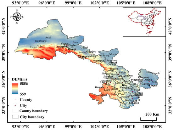
Figure 1.
Administrative map of Gansu Province.
2.2. Data
The yield and sown area of maize by county in Gansu Province from 1981 to 2020 were obtained from the Gansu Yearbook (1994–2009), Gansu Development Yearbook (2010–2021), Gansu Statistical Yearbook (1983–2021), Gansu Rural Economic Yearbook (1992–1999), and Gansu Rural Yearbook (2000–2020). By comparison, conversion, and verification, reliable maize yield statistics are gained for each county in Gansu Province.
Additionally, meteorological data are collected to analyze the impact of climate change on risks. The meteorological data were yearly precipitation and average temperature for each county from 1991 to 2020, received from the Gansu Provincial Meteorological Bureau.
2.3. Meteorological Hazard Risk Evaluation
2.3.1. Trend Yield and Relative Meteorological Yield
The maize yield series consists of trend yield (YT) and meteorological yield (YW) (Equations (1) and (2)).
where Y is the yield, YT is the trend yield, and YM is the meteorological yield. YR is the relative meteorological yield, representing the influence of meteorological factors on yield.
The trend yield is estimated using the moving average method and historical yield data from each county in Gansu Province. The meteorological yield and relative meteorological yield are calculated on this basis. The meteorological yield was then determined by the difference between unit yield and trend yield, and then the relative meteorological yield was the ratio of meteorological yield to trend yield.
2.3.2. Calculation of Risk Indicators
The trend, fluctuation, extreme yield values, and relative meteorological yields are critical components of maize risk and are all calculated based on the above yield, trend yield, and relative meteorological yield.
Thirteen risk indicators were obtained, including the trend yield tendency rate (YTs), mean yield reduction rate (YMave), maximum yield reduction rate (YMmax), mean fluctuation coefficient (YMabs), fluctuation tendency rate (YMs), the variation coefficient of yields and yield reduction rates (Ycv and YMcv), and probability of various yield reduction rates (slight, slight-medium, medium, medium-severe, severe, and total) (Psl, Pslm, Pm, Psem, Pse, and PT).
Among these, two risk indicators, the trend yield tendency rate (YTs) and the variation coefficient of yield (Yvc), can be taken from the yield series (Equations (3) and (4)). YTs is retrieved by the regression of trend yield against time, and the slope represents the tendency rate. A positive YTs implies a trend of increasing yield, while the opposite indicates a falling tendency. Yvc represents the dispersion degree of the yield. A higher Yvc value suggests more severe interannual yield changes and more unstable maize production. Yvc is typically the ratio of the standard deviation to the mean value for yield.
where YTs is the trend yield tendency rate; YT is the trend yield series; Yvc is the variation coefficient of yield; Yi is the yield in year i; is the average yield; and n is the number of year series.
Another eleven indicators can be taken from the maize relative meteorological yield series (Equations (5)–(10)).
where YMave, YMabs, and YMmax are the average yield reduction rate, average fluctuation coefficient, and maximum yield reduction rate, respectively; YMcv is the variation coefficient of yield reduction; is the average yield reduction rate; and YMs is the fluctuation tendency rate of relative meteorological yield. YM is the relative meteorological yield series; YMi is the relative meteorological yield in year i; n is the number of year series; and nym is the number of years of yield decrease.
and are the occurrence probabilities of yield reduction at (YM1, YM2, and YMi, respectively). PT, Psl, Pslm, Pm, Psem, and Pse separately refer to the occurrence probability of yield reduction (YM < 0), slight yield reduction (0 ≦ YM ≦ 5%), slight-medium yield reduction (5% < YM ≦ 10%), medium yield reduction (10% < YM ≦ 20%), medium-severe yield reduction (20% < YM ≦ 30%), and severe yield reduction (YM > 30%), respectively.
In addition, the mean values of risk indicators from 1981 to 1990, 1991 to 2000, 2001 to 2010, and 2011 to 2020 represent the interdecadal values for the 1980s, 1990s, 2000s, and 2010s, respectively. Additionally, an equal interval paired with the percentile approach is utilized for zoning, which is convenient for comparison across various decades.
2.3.3. Comprehensive Risk and Zoning
According to the meaning of each indicator and its function in risk, only eleven indicators, i.e., YTs, YMave, YMmax, YMabs, YMs, Ycv, YMcv, Psl, Pslm, Pse, and PT, are selected for maize risk assessment. Due to the disparities in the unit and absolute values, these indicators are first processed using the extreme difference standardization approach. Differentiated standardization procedures are needed because each risk indicator affects the risk result differently (Equations (11)).
where is the normalized value, is the original data, and and represent the sequence’s maximum and minimum values, respectively. The risk is highest when is 1.0, while the risk is lowest when is 0. Positive normalization is applied if rises as increases; otherwise, negative normalization is utilized. Therefore, YTs, YMave, YMmax, YMcv, Psl, and Pslm are computed according to negative normalization, whereas YMabs, YMs, Ycv, PT, and Pse are determined according to positive normalization.
A comprehensive risk assessment model for maize was created based on the above standardization indexes and the weighted average method (Equations (12)).
where Ri is the comprehensive risk value for the ith county, and and are the risk value and the weight of the jth indicator for the ith county, respectively. Here, equivalent weights (1/11) are used. The larger the Ri value is, the higher the comprehensive risk.
Finally, depending on the risk values, the K-means clustering algorithm is utilized for risk zoning. The comprehensive risk is classified into five levels: high, medium-high, medium, medium-low, and low risk. The K-means clustering algorithm can classify indicators or samples without prior knowledge and is now widely used in risk zoning.
2.4. Spatial Correlation
Moran’s I index is often used for spatial correlation analysis, which measures a variable’s clustering. Moran’s I index is divided into global Moran’s I index and local Moran’s I index [25,26,27]. The global Moran’s I index implies whether the risk indicator is spatially clustered. In contrast, the local Moran’s I index illustrates how the risk indicator is spatially clustered, i.e., where the clustering occurs and the type of clustering. Usually, local correlation is investigated when there is a global correlation present. Moran’s I index is calculated and plotted by Arcgis10.2 software. In addition, its computational complexity is also detected. The definition and calculation model of each index is as follows.
2.4.1. Global Moran’s I Index
Moran’s I index runs from −1.0 to +1.0, with larger absolute values suggesting stronger autocorrelation. A positive value of Moran’s I index indicates a positive spatial correlation and a clustering effect. The larger Moran’s I index is, the more pronounced the spatial correlation. Its negative value means a negative spatial correlation. The smaller Moran’s I index is, the more noticeable the spatial difference. When Moran’s I index is zero, it shows a random spatial distribution. The formula is as follows (Equations (13)):
where n is the county number; and are the risk indicator values for the ith and jth counties, respectively; is the spatial weight matrix for the ith and jth counties; and is the mean value of the risk indicator. The adjacency criterion is employed to create the spatial weight matrix, i.e., is one when county i is close to county j; otherwise, is zero. Moreover, the annual and decadal Moran’s I index for each risk indicator are determined.
The p and Z statistics are introduced to analyze the significance of Moran’s I index. The p-value refers to the probability. When the p-value is small, the spatial pattern is unlikely to arise from a random process. The Z value is the multiple of the standard deviation.
When > 1.65 with p < 0.10, the confidence level is 90%; when > 1.96 with p < 0.05, the confidence level is 95%; and when > 2.58 with p < 0.01, the confidence level is 99% [28].
2.4.2. Local Moran’s I Index
The local Moran’s I index measures the aggregation and divergence of risk indicators between a county and its adjacent counties. By spatial clustering, a local indicator of spatial association diagram (LISA diagram) is produced, which is further subdivided into five types: high-high clustering (H-H), low-low clustering (L-L), high-low outlier (H-L), low-high outlier (L-H), and insignificant clustering.
Generally, high-high (low-low) clustering indicates that the risk indicator values are high (low) in this county and its adjacent counties. Low-high aggregation means that the risk indicator value of a county is low and that of its surrounding counties is high, whereas it is the reverse in the case of high-low aggregation. The formula is as follows (Equations (14)):
where n is the county number; and are the risk indicator values for the ith and jth counties, respectively; is the spatial weight matrix; is the mean value of the risk indicator; and is the sum of the elements of the spatial weight matrix.
2.5. Spatial Barycenter Migration
In spatial analysis, the weighted average center of a geographical element is referred to as the barycenter. Based on the coordinates and variable values of each county, the barycenter model is established, such as the barycenter model of the yield reduction rate or risk value. The barycenter migration model can graphically reflect the regional clustering, variation, and shifting patterns of risk indicators.
For the maize risk indicators, the barycenter model is computed as follows (Equations (15)):
where X and Y are the barycenter coordinates; and are the longitude and latitude of the ith county, respectively; and is the risk indicator value of the ith county. The annual and interdecadal barycenters for the risk indicator are independently computed, which provides the trajectory of barycenter migration of maize risk.
Additionally, the distance of barycenter migration between two periods is calculated (Equations (16)–(18)).
where , , and represent the migration distance of the barycenter, longitude, and latitude between the ith and jth decade, respectively; and refer to longitude and latitude, respectively; and C is a constant with a value of 111.111, which converts geographic coordinate units (1°) into plane distances (km).
2.6. Time Series Diagnostic Analysis
The Mann-Kendall (M-K) trend test and Hurst index are used to diagnose the time-series features of relevant risk indicators.
Mann-Kendall tests [29,30] were carried out to detect trends and changes in disaster loss over the years of analysis. The M-K test has the benefits of being simple, not needing the sample to follow a specific distribution, and not being affected by a few outliers. Sen’s slope values were used to understand the trend of disaster loss change from 1981 to 2020. Equations (19)–(22) define the trend tests and slope value computation [31,32,33,34].
here Xi and Xj are chronologically placed values of variables in the time series, n represents the observation count, ties for pth value is shown as tp, and tied values number is shown as q. The MATLAB program is used to carry out the M-K test, and a statistical value expressing the trend (Z value) is generated.
Generally, when Z > 0, the time series of the risk indicator displays a rising trend; when Z < 0, the time series exhibits a declining trend. In addition, the precise value of Z is used to determine whether this trend is significant. When |Z| is greater than 1.28, 1.64, and 2.32, it signifies passing the significance test with 90%, 95%, and 99% confidence levels, respectively.
The Hurst index (H) describes the trend sustainability of the time series. When H = 0.5, the time series is entirely independent; when 0 < H < 0.5, it implies that future changes are the reverse of the past trend; when H > 0.5, it means that future changes are consistent with the past trend. The larger the H value is, the stronger the sustainability [35].
2.7. Influence of Climate Elements on Comprehensive Risk
Furthermore, the effects of climate elements on comprehensive risk were investigated, mainly considering the effects of precipitation and temperature.
The meteorological factors include annual precipitation (p) and annual mean temperature (T), as well as the yearly precipitation anomaly percentage (Pa) and annual mean temperature anomaly percentage (Ta) (Equations (15) and (16)).
Precipitation anomaly percentage:
Annual mean temperature anomaly percentage:
where and are the precipitation anomaly percentage and annual mean temperature anomaly percentage, respectively; P and T are the yearly precipitation and mean temperature, respectively; and and are the average values of rainfall and temperature for 1981–2020, respectively.
3. Results
3.1. Spatial and Temporal Distribution of Maize Production Risk
3.1.1. Maize Trend Yield
The interdecadal variations in maize trend yield are illustrated in Figure 2. In the 1980s, the trend yields of 60.87% of counties are less than 4000 kg/hm2, mainly in areas south of Wuwei City. However, 24.64% of counties have a trend yield exceeding 5000 kg/hm2, mainly in the north of Zhangye. In the 1990s, the maize trend yield improves dramatically. The county percentage below 4000 kg/hm2 drops to 40.28%, while the ratio surpassing 5000 kg/hm2 reaches 44.44%. In the 2000s, only 23.6% of counties have trend yields below 4000 kg/hm2, and 70.83% of counties with yields above 5000 kg/hm2 are in Zhangye and Jiuquan. In the 2010s, all counties have trend yields exceeding 3000 kg/hm2. Only 12.50% of counties have trend yields below 4000 kg/hm2, and the county percentage surpassing 5000 kg/hm2 reaches 75.0%. Overall, the trend yield in Gansu is lower in the southern counties and higher in the northern counties.

Figure 2.
Spatial and temporal variation in maize trend yield.
3.1.2. Yield Reduction and Fluctuation Characteristics of Maize
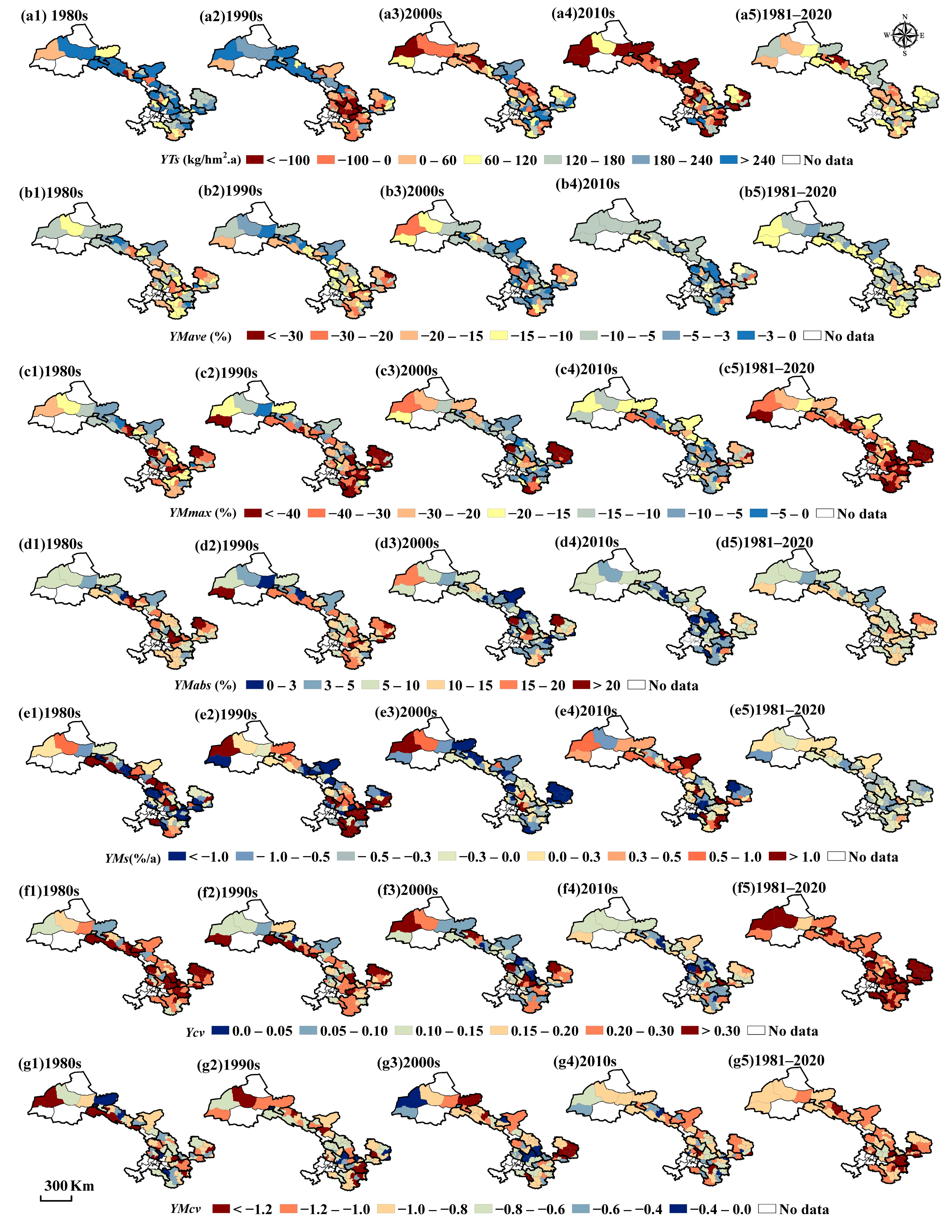
The spatial and temporal distribution of the maize trend yield tendency rate is illustrated in Figure 3a1–a5. In the 1980s, 1990s, 2000s, and 2010s, the maize trend yield tends to increase for 95.7%, 59.7%, 76.4%, and 38.9% of counties, respectively, whereas it has a significant falling trend for 1.4%, 15.3%, 8.3%, and 38.9% of counties (less than −100 kg/hm2·a). Except for six counties, the trend yields in most counties generally rises from 1981 to 2020. Most regions in Longnan City have a low trend yield increase rate of less than 60.0 kg/hm2, while most areas in Wuwei and Tianshui City have a higher increase rate (more than 120.0 kg/hm2.a).
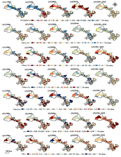
Figure 3.
Spatial and temporal distribution of maize yield reduction and fluctuation.
The variation in the maize yield reduction rate is displayed in Figure 3b1–b5. The mean yield reduction rates of maize in Gansu Province are −11.8%, −12.6%, −8.7%, and −8.5%, and the county proportions with average yield reduction rates at [0, 10%] interval are 42.0%, 43%, 72.4%, and 69.4% in the 1980s, 1990s, 2000s, and 2010s, respectively. In the 1980s, it is higher (more than 10%) in most counties. In the 1990s, it increases in 50.72% of counties. There are more significant increases of over 15% in five counties. In the 2000s, it fell in 65.28% of counties and substantially dropped to less than 15% in most counties. Among them, three counties have more significant declines (more than 20%), while four counties see an increase (more than 10%). In the 2010s, eleven counties see a notable decline of more than 10%, while ten counties rose more than 10%. Overall, the regions with higher yield reduction are located in southern and eastern Gansu.
The maximum yield decrease rate signifies encountering catastrophe, as shown in Figure 3c1–c5. In the 1980s, 1990s, 2000s, and 2010s, the county proportions exceeding 40% are 9.7%, 25.0%, 12.5%, and 2.8%, respectively. Catastrophes occur largely in eastern and southern Gansu. From 1981 to 2020, 70.8%, 36.1%, and 18.1% of counties suffer catastrophes with maximum yield reduction rates of more than 30%, 40%, and 50%, respectively.
The average fluctuation coefficient illustrates the sensitivity of yield to climatic influences (Figure 3d1–d5). In the 1980s, 1990s, 2000s, and 2010s, it is 11.1%, 12.1%, 7.6%, and 6.5% for the whole province, and the county proportions of the average fluctuation coefficients at [0, 10%] interval are 47.83%, 41.66%, 73.61%, and 81.94%, respectively. In the 1990s, 50.72% of counties increase, and 9.7% see a rise of more than 10%. In the 2000s, maize yield fluctuations significantly reduced in 70.83% of counties, and most counties had a mean fluctuation coefficient of less than 15%. In the 2010s, it decreased in 54.17% of the counties and even fell below 10% in most regions. Six counties exhibit considerable decreases (more than 10%). Overall, from 1981 to 2020, the counties with severe fluctuations are mostly located in Dingxi and Qingyang cities.
The fluctuation tendency rate is depicted in Figure 3e1–e5. In the 1980s, 1990s, 2000s, and 2010s, the county proportions with positive fluctuation tendency rates are 30.4%, 59.7%, 26.4%, and 59.7%, respectively. From 1981 to 2020, 26.39% of the counties have a positive fluctuation tendency rate and are predominantly found in northeastern Gansu. Eleven counties have tendency rates less than −0.45%/a, with fluctuating trends swiftly reducing and maize production gradually stabilizing.
The yield variation coefficient of Gansu Province was 0.267, 0.206, 0.166, and 0.139 in the 1980s, 1990s, 2000s, and 2010s, respectively (Figure 3f1–f5). Overall, from 1981 to 2020, regions with significant variation coefficients are found in Qingyang and eastern Dingxi, indicating that their yields wildly fluctuate and are very unstable.
The variation coefficients for yield reduction are given in Figure 3g1–g5. In the 1980s, 1990s, 2000s, and 2010s, it is −0.811, −0.851, −0.838, and −0.807 for the entire province, respectively, while the county proportions with variation coefficients for yield reduction above −1.2 are 13.0%, 15.3%, 15.3%, and 5.6%, respectively. Overall, in the last 40 years, areas with large fluctuations in yield reduction rates are distributed in Tianshui City and the border areas of Pingqing. Comparatively, it in seven counties is between [−0.80, 0], and these counties have had minimal change in disaster loss. They can be prepared to cope with disaster resistance according to previous situations.
3.1.3. The Occurrence Probability of Maize Yield Reduction Rate
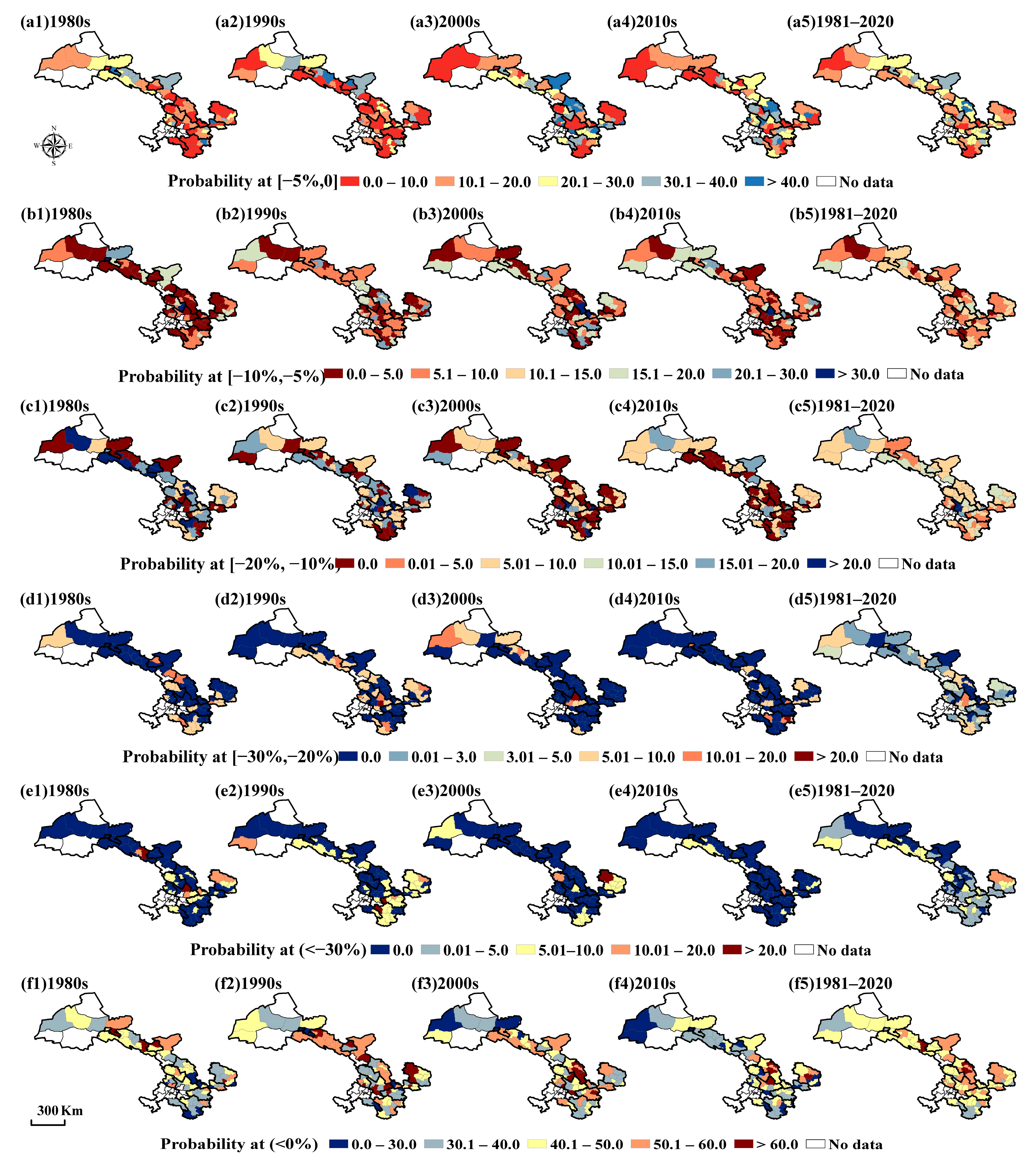
The occurrence probability of different maize yield reduction rates in each county of Gansu Province is presented in Figure 4.
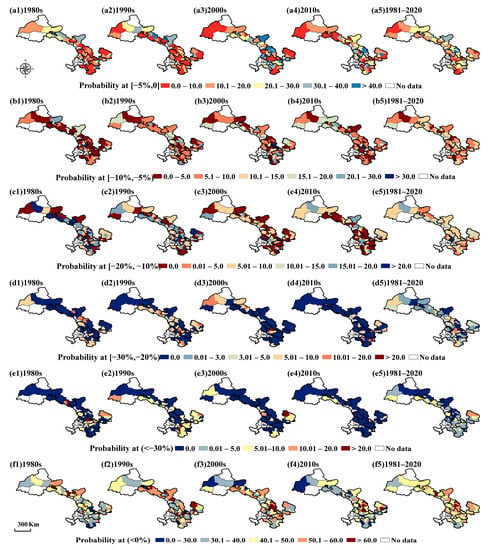
Figure 4.
Spatial and temporal distribution of the probability of maize yield reduction.
The county proportions with a probability in [0, 5%] of more than 20% are 29.0%, 27.8%, 54.2%, 40.3%, and 52.1% in the 1980s, 1990s, 2000s, 2010s, and 1981–2020, respectively (Figure 4a1–a5). The range of the counties prone to slight yield loss considerably expands after 2000. Overall, from 1981 to 2020, eleven counties have a slight yield loss probability of over 30% located in east-central Gansu, while six counties have a lower probability (less than 10%).
The county proportions with a probability in (5%, 10%] of more than 15% are 23.2%, 29.2%, 30.6%, 25.0%, and 9.7% in the four decades and 1981–2020, respectively (Figure 4b1–b5). The areas prone to slight-medium yield loss have changed little in the last 40 years. Prone areas include Yuzhong, Huining, Gaotai, Lingtai, Jingning, Aksai, and Guanghe counties.
The county proportions with a probability in (10%, 20%] of more than 15% were 37.7%, 33.3%, 13.9%, 12.5%, and 6.9% in the above five time intervals, respectively (Figure 4c1–c5). The extent of medium yield reduction significantly decreases after 2000. The vulnerable areas are distributed in Zhuanglang, Anxi, Weiyuan, Lintao, and Zhang counties, while eleven counties have a low occurrence probability (less than 3%).
For the yield reduction rate of (20%, 30%] interval, the county proportions with an occurrence probability of more than 5% are 31.9%, 40.3%, 15.3%, 23.6%, and 22.2% in the five time intervals, respectively (Figure 4d1–d5). The range that is prone to medium-severe yield loss decreases significantly after 2000. Sixteen counties belong to the prone areas. However, 20.83% of counties do not experience medium-severe disasters, mainly in Baiyin and Tianshui cities.
The maize yield reduction rate probability exceeding 30% is illustrated in Figure 4e1–e5. The percentage of counties with a probability of yield drop surpassing 30% being higher than 5% was 34.8%, 44.4%, 20.8%, 9.7%, and 22.2% in the 1980s, 1990s, 2000s, 2010s, and 1981–2020, respectively. The percentage of counties where no severe yield drop occurred is 65.2%, 55.6%, 79.2%, 90.3%, and 29.2% in the above five periods. In the 1980s, the counties prone to severe yield reduction were located in central Gansu, while it was situated in southern Gansu in the 1990s and eastern Gansu in the 2000s. In the 2010s, the number of regions with catastrophes dramatically decreases. Overall, from 1981 to 2020, the areas prone to severe yield reduction are located in the east-central part of Gansu, and sixteen counties have an occurrence probability of more than 5%. In contrast, 29.2% of counties do not experience heavy yield reductions.
3.1.4. Time-Series Variation in Disaster Loss at the Provincial Scale
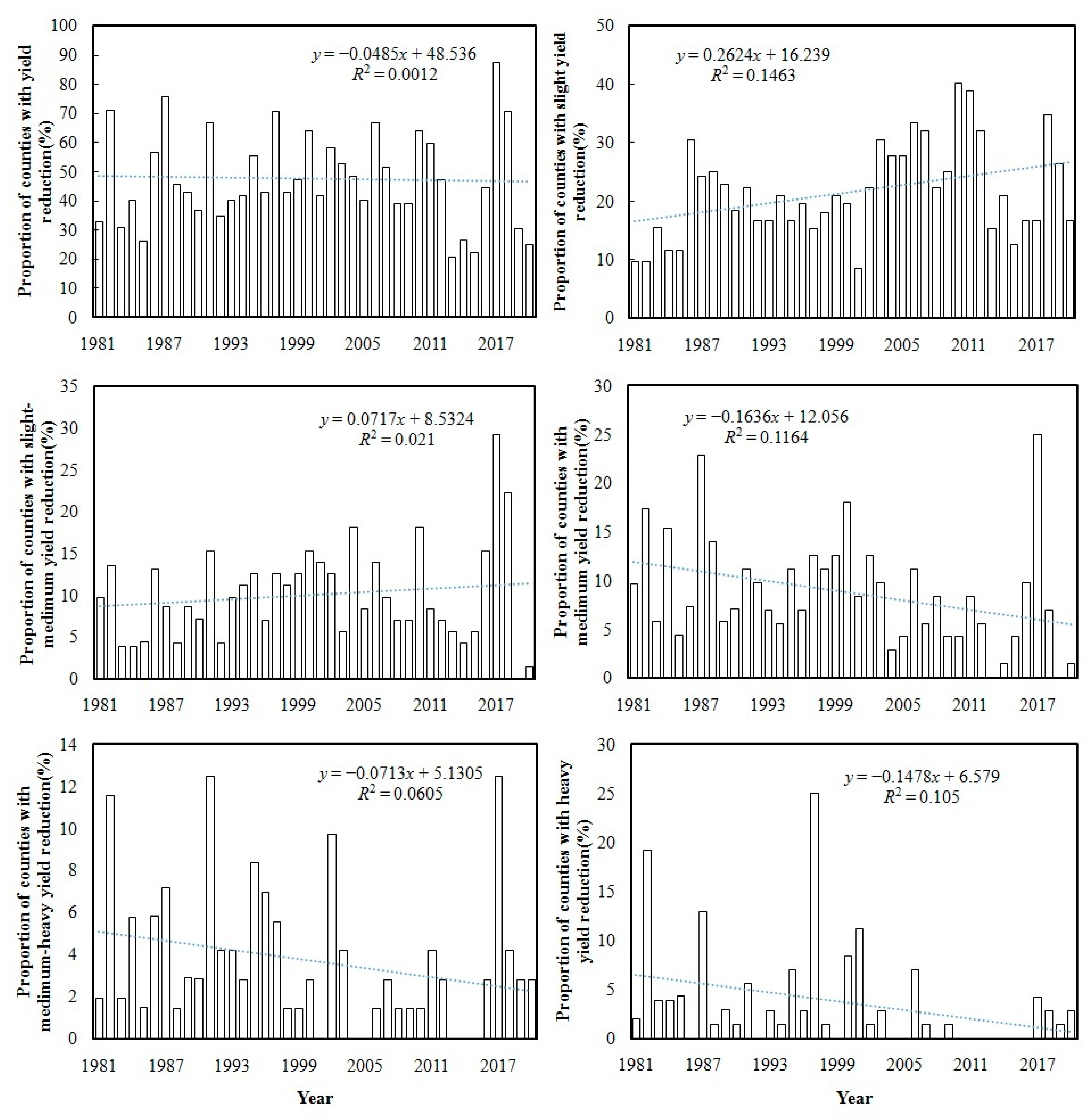
The interannual variations in the county proportions for various yield losses are depicted in Figure 5. The county proportions with medium and severe yield reduction show a significant downward trend from 1981 to 2020, whereas the proportion with slight yield reduction displays a significant upward trend. Furthermore, the fractions with slight-medium and medium-severe yield reductions individually exhibit weaker increasing and decreasing trends.
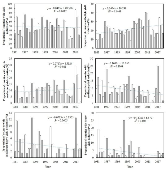
Figure 5.
Interannual variation in county proportions with varying disaster losses.
The county proportion with severe yield reduction is higher before 2006 and after 2017, with peaks in 1982, 1987, 1997, and 2001, particularly in 1997, when 25% of Gansu Province’s counties faced a catastrophe. The proportion of counties with medium-severe yield reduction peaks are in 1982, 1991, 1995, 2002, and 2017. Overall, 2013–2015 are harvest years with no more than medium-severe yield losses. Harvests were slightly poor in 1988–1999, 2004–2005, 2008–2010, and 2012–2016, with no more than 3% of counties seeing medium-severe or severe yield reductions.
There are two distinct phases for the fraction variation of counties with slight and slight-medium yield declines. From 1986 to 2001, the fraction of counties with a slight yield reduction tended to decrease, while that with a slight-medium yield reduction tended to grow. However, from 2001 to 2012, the situation is reversed.
Overall, in most years, the proportion of counties with increased yield is higher than that with decreased yield. Only 15 years have had a higher proportion of counties with reduced yields. Most counties suffered disasters in 1982, 1987, 1991, 1997, 2000, 2006, 2010, 2017, and 2018, with yield reduction counties accounting for more than 60%. In particular, maize yield fell in 87.5% of counties in 2017.
3.1.5. Spatial and Temporal Variation in Maize Production Risk
The spatial and temporal distribution features of maize production risk zoning in Gansu Province are illustrated in Figure 6. According to the K-means clustering algorithm, most counties belong to the medium-low or low-risk zones.

Figure 6.
Spatial and temporal distribution of maize production risk.
The percentages of high, medium-high, medium, medium-low, and low-risk counties in the 1980s are 7.2%, 11.6%, 18.8%, 37.7%, and 24.6%, respectively, with high-risk counties including Anding, Tongwei, Shandan, Huan, and Longxi. In the 1990s, the proportions are 1.4%, 17.4%, 33.3%, 33.3%, and 18.8%, and only Wushan County belongs to the high-risk zone. In the 2000s, those are 5.8%, 11.6%, 17.4%, 24.6%, and 44.9%, with high-risk counties containing Huan, Dunhuang, Yongdeng, and Anding. In the 2010s, the proportions are 1.4%, 8.7%, 13.0%, 40.6%, and 40.6%, with Jingning County being the only high-risk county.
Overall, from 1981 to 2020, high, medium-high, medium, medium-low, and low-risk counties account for 7.2%, 26.1%, 26.1%, 26.1%, and 18.8%, respectively, with high-risk counties comprising Huan, Huachi, Jingning, Yongdeng, and Anding. Over the last 40 years, high-risk counties have been primarily found in Qingyang and Longnan cities, as well as in northern Tianshui and southern Dingxi cities. Low-risk counties are mostly found in Wuwei and Zhangye cities along the Hexi Corridor.
3.2. Spatial Correlation of Maize Risk Indicators
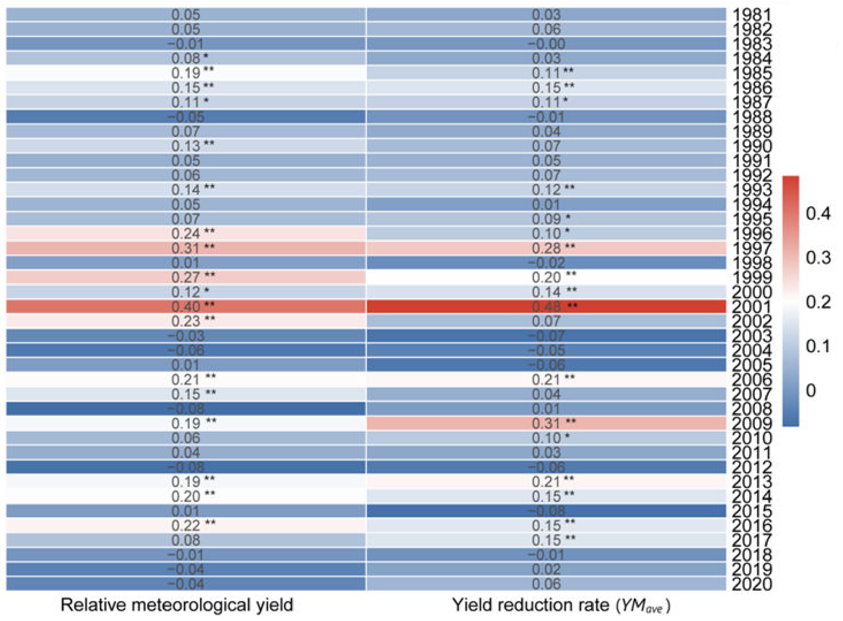
The global Moran’s I indexes for each indicator in each decade and the relative meteorological yield and yield reduction rate for each year are calculated to determine whether and how the risk variables of maize production are geographically aggregated (Figure 7). In Figure 7, the asterisk (*) and double asterisk (**) respectively represent achieving 95% and 99% confidence levels, while the others is insignificant.
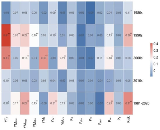
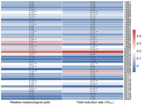
Figure 7.
Temporal variation in the spatial correlation of maize risk indicators. (* and ** indicate reaching the 95% and 99% confidence levels, respectively).
Next, to examine the aggregation type, the local Moran’s I index was generated for indicators and periods with significant aggregation (Figure 8).
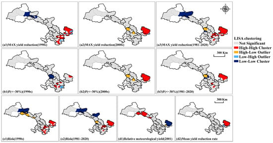
Figure 8.
LISA clustering diagram for maize risk variables.
3.2.1. Global Moran’sMoran’s I Index Calculation
The global Moran’s I indexes for each risk indicator over the decades are displayed in Figure 7. Moran’s I indexes for most indicators are greater than zero, suggesting a distinct geographical aggregation of maize disaster loss risk in Gansu Province. Among them, nine risk variables, YTs, YMave, YMmax, YMabs, YMs, Ycv and YMcv, Pse, and risk level, have more significant spatial aggregation with a confidence level over 90% in most decades.
The global Moran’s I index displays apparent interdecadal variations (Figure 7). Among them, the trend yield tendency rate for the 1990s and 2000s, maximum yield reduction rate for 1981–2020, fluctuation tendency rate for the 2000s, and comprehensive risk values for the 1990s and 1981–2020 all show extremely significant aggregation, with Moran’s I index exceeding 0.25 and p-values less than 0.01. This indicates that the spatial distribution of these indicators over these periods has a strong positive correlation at the 99% confidence level. As the spatial distributions are clustered, the catastrophe loss, fluctuation tendency, and riskiness of maize production are more similar. The more discrete the spatial distributions, the more different the trends, fluctuations, extreme values, and riskiness. This also implies that the maize production risk in Gansu Province has two spatial clustering levels: high-high clustering areas with high risk or heavy disaster loss and low-low clustering areas with low risk or slight disaster loss.
The interannual variation in the global Moran’s I index for relative meteorological yields and yield reduction rates was also investigated (Figure 7). The Moran’s I indexes are greater than 0.2 for the relative meteorological yield in 1996–1997, 1999, 2001–2002, 2006, 2014, and 2016, and for the yield reduction rate in 1997, 2001, 2006, 2009, and 2013, which suggests that these two indicators have strong spatial aggregations in those years. Additionally, the years with large spatial aggregations are primarily found in the 1990s. The global Moran’s I index is less than 0.2 in other periods, implying a weak spatial relationship across the counties’ disaster losses and a high degree of fragmentation in the spatial distribution of disaster risk.
Additionally, the computational complexity of this index is explored. There were four cores and 8.00 GB of memory in the present investigation. Every calculation of the global Moran’s I index took 0.44 s on average. Because there are 14 indicators, 5 periods, and a total of 30.8 s spent, the speed is still very fast.
3.2.2. Calculation of the Local Moran’s I Index and LISA Clustering Diagram
The LISA clusters for the risk variables (maximum yield reduction rate, probability of severe yield reduction, and risk) and three periods (the 1990s, 2000s, and 1981–2020) are presented in Figure 8.
The maximum yield reduction rates in Yumen, Jiayuguan, Suzhou, and Gaotai display a low-low aggregation pattern only in the 1990s, suggesting that the maximum yield reduction rates are small in these counties. On the other hand, the high-high aggregation pattern is observed in Pingliang and Qingyang cities, indicating that this region and surrounding areas have high yield reduction rates and that the aggregation area expanded from the 1990s to the 2000s. Moreover, several low-low clustering areas are scattered in southern Gansu’s Longnan and Tianshui cities in the 1990s.
The probability of severe yield reduction has a low-low aggregation zone in the 1990s in Lanzhou city and a high-high aggregation zone in the 2000s in Qingyang city. Furthermore, the spatial aggregation of the probability of heavy yield reduction changed, with Lanzhou City shifting from a low-low aggregation area in the 1990s to a high-low aggregation area in the 2000s. In addition, the high-high aggregation area in Qingyang City significantly expands from a sporadic distribution in the 1990s.
The clustering of the comprehensive risk is similar to that of the risk indicators. In the 1990s, there was a low-low aggregation zone in the southern part of Jiuquan with low risk and a high-high aggregation area in Qingyang City with high risk.
The yearly clustering of the yield reduction rate is also similar to the interdecadal distribution of risk indicator aggregation.
In general, the spatial clustering of most risk variables has changed little over the last 40 years.
Additionally, using the same computer configuration, we tested the complexity of the local Moran’s I index calculation. Every calculation of the local Moran’s I index took 8.35 s on average. Because it takes 10 calculations, it takes a total of 83.5 s. Comparatively speaking, the calculation of local Moran’s I index is more complicated. If there are more indicators or calculations, it needs to be run on a better-configured computer.
3.3. Spatial and Temporal Variation in the Maize Risk Variable Barycenter
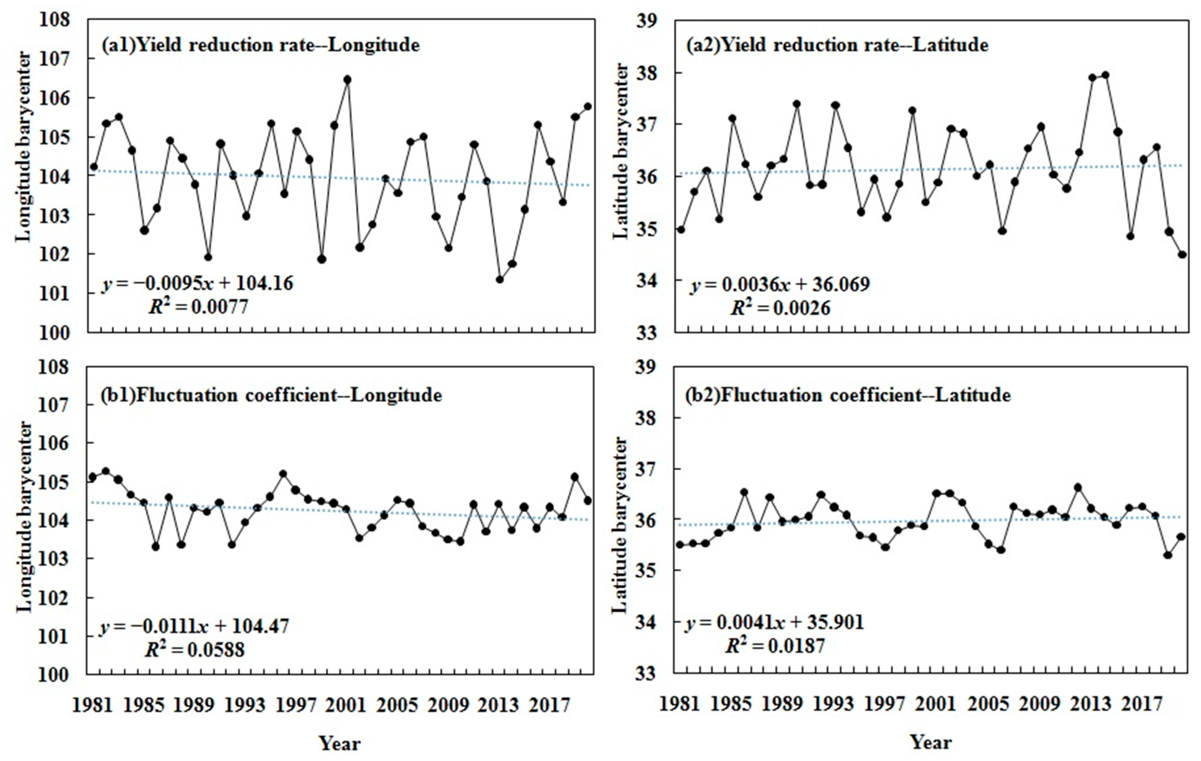
To further explore the geographical variation in maize disaster loss risk, the movement of risk indicators is decomposed into two directions: longitude and latitude (Figure 9). The geographic barycenter of the yield reduction rate exhibits considerable interannual fluctuations in both longitude and latitude, with large fluctuations in longitude between 101° and 107° and latitude between 34° and 38°. Overall, the barycenter has a slight downward trend in longitude and a slight upward trend in latitude, indicating a tendency for the yield reduction barycenter to move to areas of lower longitude and higher latitude (Figure 9a1,a2).
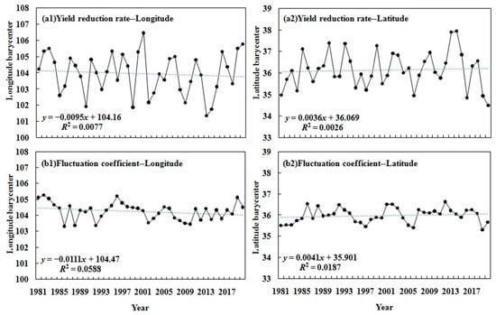
Figure 9.
Interannual variation in the longitude and latitude of the barycenter for the yield reduction rate and fluctuation coefficient.
The barycenter’s interannual variation in longitude and latitude for the fluctuation coefficient is slight. The longitude and latitude of the barycenter only slightly vary at 103°–106° and 35°–37°. From the whole period, the barycenter exhibits a slight longitude decrease and latitude increase movement, with a general trend toward the northwest, which is similar to the yield reduction rate (Figure 9b1,b2).
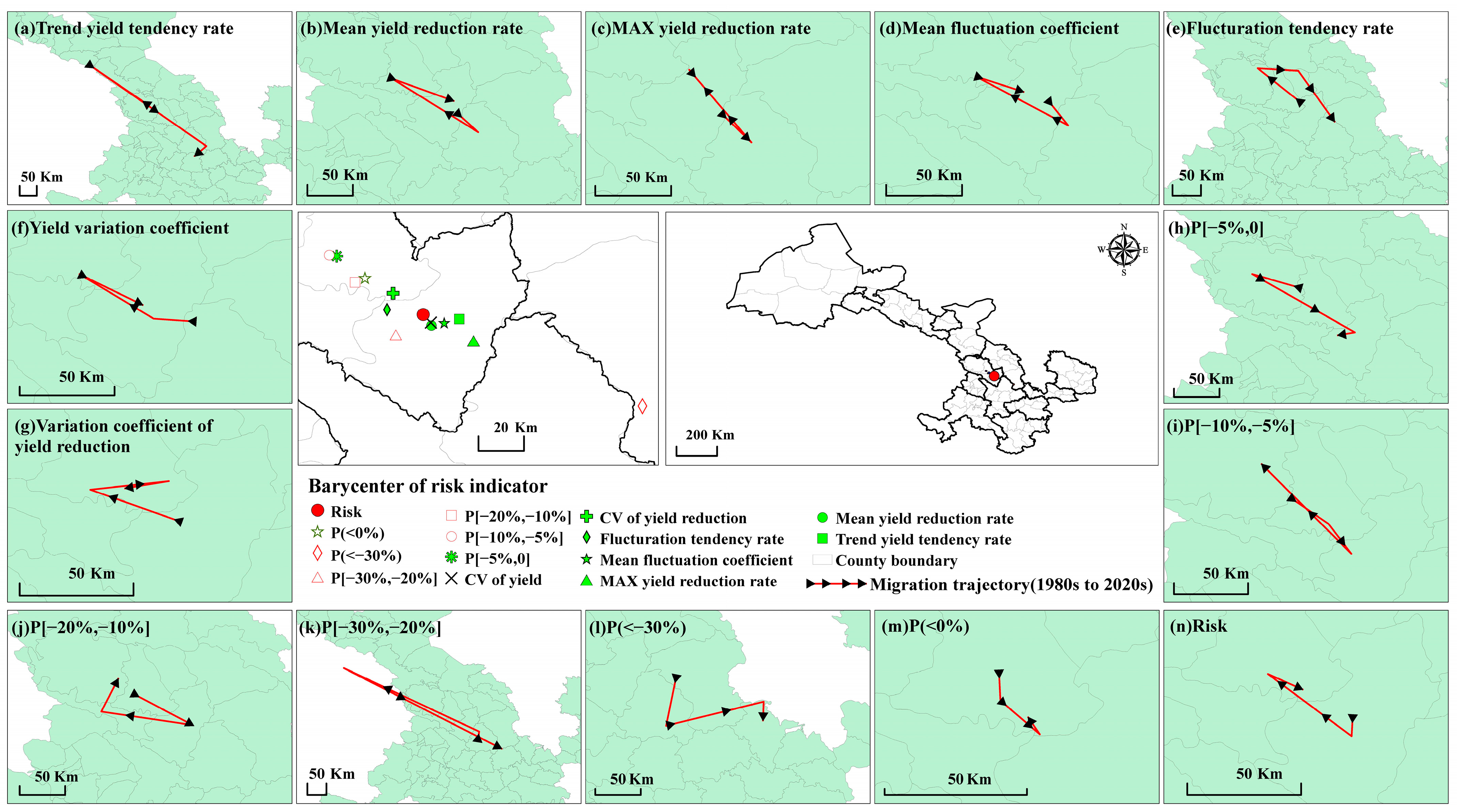
The geographic coordinates of the barycenter are calculated for each risk indicator in each decade, and then its migration trajectory along the 1980s–1990s–2000s–2010s is plotted (Figure 10). The barycenters of most risk variables are situated in Lanzhou City, with only the barycenter for the probability of severe disasters in Huining County. In addition, the geographical distributions of barycenters for indicators are uneven, and their migrations are complicated. Most indicators shifted along the northwest-southeast line. However, there are significant differences in the direction and distance of movement.
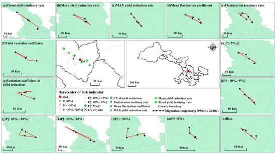
Figure 10.
Migration trajectory of the barycenter of maize risk indicators from the 1980s to the 2000s.
From the 1980s to the 1990s, four risk indicators, i.e., the trend yield tendency rate, fluctuation tendency rate, variation coefficient of yield reduction, and probability of slight yield reduction, migrated to the northwest. The yield variation coefficient migrated to the west. On the other hand, the probability of total, medium-severe, and severe yield reduction independently tended to migrate to the south, north, and southwest, respectively. The other risk indicators (YMave, YMmax, YMabs, Pslm, and Pm) shift to the southeast. To summarize, most indicators have a southward movement trend. The overall risk tends to move southward, but the migration distance is short.
From the 1990s to the 2000s, five indicators (YMave, YMmax, YMabs, Ycv, and Psem) migrate northwestward; five indicators (YTs, YMs, PT, Psl, and Pslm) migrate southeastward; two indicators (YMs and Pse) migrate eastward; and the other indicators (YMcv and Pm) separately tend to migrate northeastward and westward. However, the overall risk has a trend of northwestward migration, with a longer movement distance.
From the 2000s to the 2010s, six indicators (YMave, YMmax, YMabs, YMs, Ycv, and Psem) show a trend to migrate to the southeast. In contrast, two indicators (YTs and YMcv) tend to migrate to the southwest. Furthermore, the other five indicators (PT, Psl, Pslm, Pm, and Pse) tend to migrate to the north, west, northwest, northeast, and south, respectively. Nine indicators tend to shift southward. The overall risk tends to move back toward the southeast, but the migration distance is comparatively shorter.
In addition, the migration distances of the barycenter for each indicator are calculated (Table 1).

Table 1.
Migration distances of the barycenter for each risk indicator over time.
From the 1980s to the 1990s, the risk indicators with the farthest migration distances for longitude and barycenter are YTs, YMs, and Pm. Those for latitude were YTs, YMs, and Pse. However, the risk indicator with the shortest longitude, latitude, and barycenter migration distances are Pse, YMcv, and Ycv, respectively. Longitude migration has a greater impact on barycenter migration.
From the 1990s to the 2000s, the top three risk indicators with the farthest longitude, latitude, and barycenter migration distances are YTs, Psl, and Psem. In addition, those with the shortest migration distances for longitude and barycenter are PT, Pslm, and YMcv. In contrast, those for latitude are PT, YMs, and YMcv. Latitudinal migration has a more significant impact on barycenter migration.
From the 2000s to the 2010s, the risk indicators with the farthest migration distances for longitude are Psem, YMave, and YMs. Furthermore, those for latitude and barycenter are Psem, Pslm, and YMs. In contrast, the indicators with the smallest migration distances for longitude are YMmax, PT, and Pse; for latitude, are YMmax, Psl, and YMcv; and for barycenter, are PT, Psl, and YMmax. The impact of latitudinal migration is comparatively more significant.
YTs, Psem, and Ycv are the top three risk indicators with the farthest longitude migration distances from 1981 to 2020. Those for latitude and barycenter are YTs, Psem, and Pse. Moreover, the indicators with the smallest distances for longitude are PT and Pslm; for latitude, are YMave, YMabs, and YMmax; and for barycenter, are YMabs, PT, and YMmax. Overall, the latitudinal migration effect is more pronounced.
In general, the migration distance of comprehensive risk is short. Latitudinal migration has a more significant impact on barycenter migration. YTs, Psem, and YMs migrate far, and their barycenter location is significantly altered. However, PT, YMmax, and YMcv have a slight shift distance.
3.4. Spatial Distribution of Variation Trends in Maize Risk Indicators
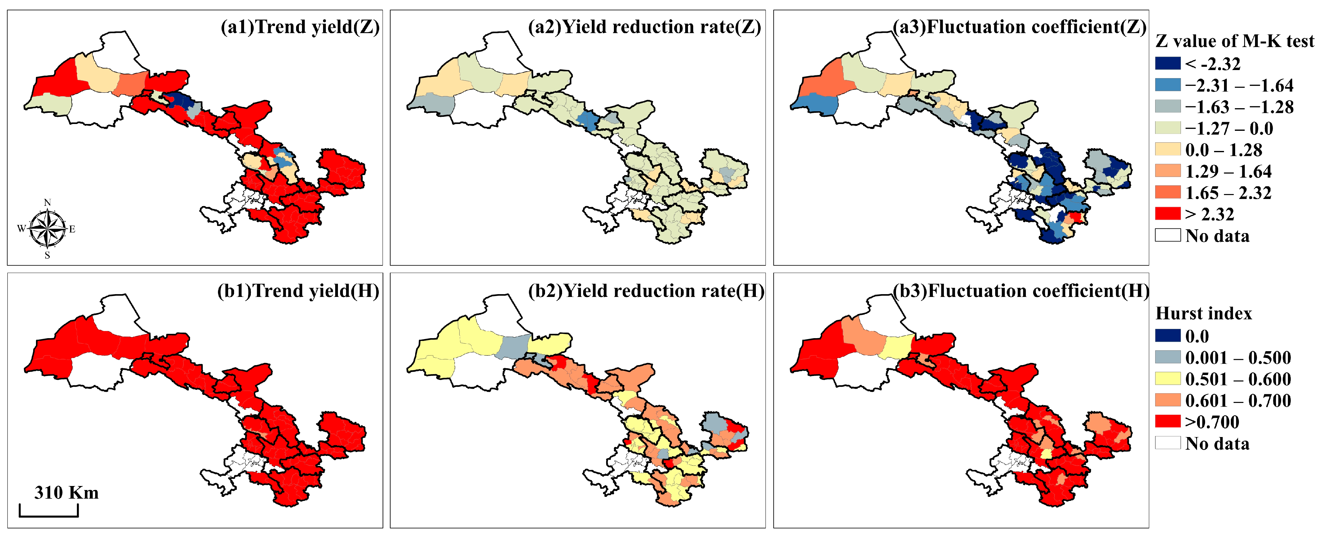
M-K tests were performed on the time series data of maize trend yield, yield reduction rate, and fluctuation coefficient from 1981 to 2020 to acquire more detailed trends in risk indicators (Figure 11a1–a3). The maize trend yields in 81.94% of counties exhibit an extremely significant increasing trend (Z > 2.32). Only Jingyuan, Linze, and Gaotai counties show a significant or extremely significant decreasing trend.
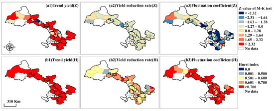
Figure 11.
Variation trend in the maize yield components and the spatial distribution of the Hurst index from 1981 to 2020.
In contrast, the yield reduction rates and fluctuation coefficients show an insignificant declining trend in most counties (−1.28 < Z < 0). For the fluctuation coefficient, 47.22% and 34.72% of counties separately show significant and extremely significant decreasing trends, while 22.2% of counties show an increasing trend, and only two counties show a significant increasing trend.
In addition, the sustainability of these trends is analyzed (Figure 11b1–b3).
The Hurst indexes of trend yield are all greater than 0.5, and 98.6% of counties have a Hurst index of over 0.7, indicating that their future short-term changes are consistent with past trends and that most counties’ trend yields will continue to rise.
For the yield reduction rate, its Hurst index is greater than 0.5 in 88.9% of the counties, with 80.5% having a Hurst index between 0.5 and 0.7, suggesting that the yield reduction trend in these counties will be weaker sustainability. Combined with the results of the M-K test, it can be deduced that the yield reduction rate in Ning County will continue to rise. Additionally, eight counties have a Hurst index of less than 0.5, indicating that their future trends in yield reduction rate are contrary to the past trend. It can be inferred that the yield reduction rate in Zhuanglang and Yumen initially displayed a rising trend but will probably turn to a falling trend in the future.
The Hurst indexes of the fluctuation coefficient in all counties are greater than 0.5, with 83.3% of counties greater than 0.7. According to the M-K trend test, it will likely continue to increase in 18.1% of counties and decline in 65.3% of counties.
Finally, the variation trends and their sustainability of county proportions with different disaster losses are thoroughly examined (Figure 12). It can be shown that the county proportions with slight and slight-medium yield reduction tend to increase (Z > 0), especially those with slight yield loss displaying a significant increase (Z > 1.64). However, the county percentage with medium, medium-severe, and severe yield reductions, as well as the total yield reduction, all present a decreasing trend (Z < 0), especially those with medium and severe yield loss showing an extremely significant decrease (Z < −2.32) and those with medium-severe yield loss having a significant decreasing trend (Z < −1.64).

Figure 12.
Variation trend and its sustainability for county proportions with different disaster losses.
The Hurst indexes of county proportions with different disaster losses are all more than 0.5, indicating that the future changes in disaster situations in Gansu Province will be consistent with the past trend. Among them, the Hurst indexes of the slight, medium, and medium-severe all surpass 0.7, demonstrating a strong continuity. Combined with the M-K test, this indicates that in the future, the scope of slight yield loss of maize will continue to expand, while that of medium and medium-severe yield reduction will continue to shrink.
3.5. Influence of Climate Elements on Comprehensive Risk
The effects of meteorological factors on risk indicators in Gansu Province are explored to reveal the impact of climate change on maize production risk. Additionally, variations of this effect over time are also investigated.
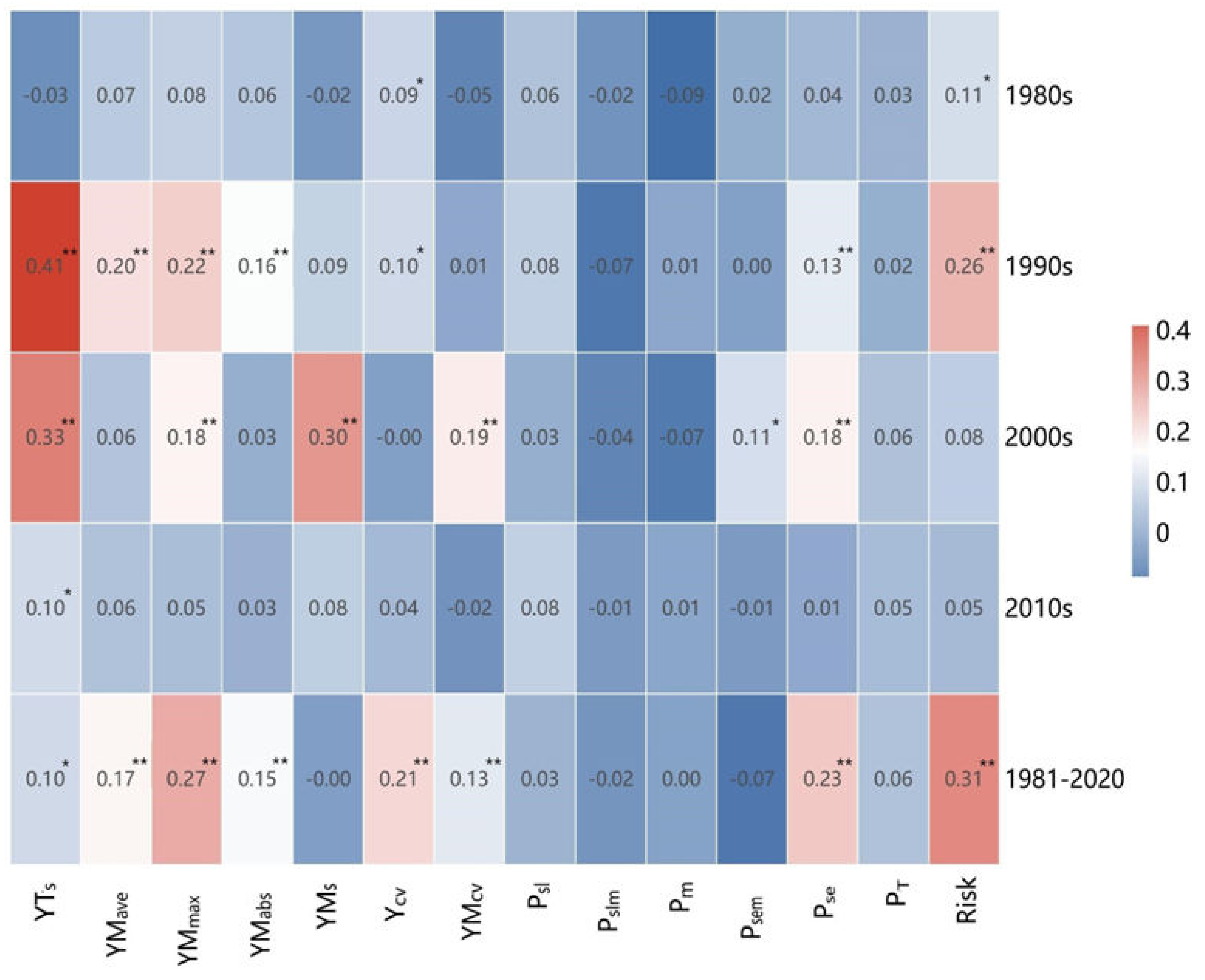
The correlations between risk indicators and meteorological factors for maize production in the different decades are presented in Figure 13. As shown, annual precipitation is significantly or very significantly correlated with most risk indicators and the comprehensive risk level in the 1990s and 2010s, as well as from 1981–2020. Additionally, the effect of precipitation amounts is higher than that of precipitation fluctuations. However, rainfall positively correlates with risk, and regions with higher rainfall also have higher risks, primarily due to the region’s characteristics.
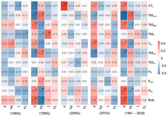
Figure 13.
Correlations between risk indicators and meteorological factors for maize production in the different periods. (* and ** indicate the significant correlation at the 0.05 level and at the0.01 level, respectively.)
Furthermore, the meteorological factor is significantly correlated with trend yield tendency rate (YTs), mean yield reduction rate (YMave), maximum yield reduction rate (YMmax), mean fluctuation coefficient (YMabs), the probability of severe yield reduction (Pse), especially in the 1990s, indicating that meteorological factor significant influence of the maize disaster loss of that era.
4. Discussion
Agro-meteorological hazards have frequently occurred worldwide in recent years and have become a significant impediment to sustainable agricultural development. Disaster risk assessment is a helpful tool for disaster prevention. Therefore, carrying out a risk assessment can effectively reduce the blindness of agricultural production and lower meteorological disaster losses, which is of great significance for food security.
The disaster loss method was chosen to assess the risk of maize production after weighing the benefits and drawbacks of various risk assessment techniques. Simultaneously, a risk evaluation index system was built by utilizing various characteristics of disaster losses. Furthermore, extensive research was conducted on the temporal and spatial features of maize production risks.
Previous studies conducted risk analysis primarily at provincial or municipal levels [36,37,38,39], with too low a spatial resolution to make well-targeted disaster prevention measures. Therefore, a refined risk assessment of maize production on a county scale was carried out here.
Second, previous assessment indicators of disaster loss were overly single, such as using only the yield reduction rate, making it difficult to fully present the issues in agricultural production [40,41]. An overall picture of the comprehensive risk of maize production under long-term yield trends, conventional disasters, and catastrophes is presented here by considering characteristics such as trends, tendencies, fluctuations, dispersions, and extremes of disaster losses.
Third, past studies were mainly static risk assessments based on historical data [42,43]. By analyzing the interdecadal variations, we dynamically evaluated the temporal evolution of maize production risk. Our findings also clearly show significant changes in risk areas over time. In addition, the M-K test and the Hurst index were used to examine the variation trend and future sustainability of risk indicators, which may provide some evidence of the impact of climate change on maize production risk.
Compared to traditional risk factor assessment technology, the disaster loss method has simple data requirements, easy operation, and high feasibility. At the same time, the new idea of combining trend, fluctuation, and extreme value can more completely and objectively identify high-risk areas of maize disaster loss.
Moreover, the findings can also reveal some points to consider: first, the high-risk maize areas are situated in southeastern Gansu, such as Qingyang, Tianshui, and Longnan cities, whereas Jiuquan City and the areas along the Hexi Corridor are low-risk areas. This is in line with the characteristics of disaster loss [36,44]. However, the Qingyang and Longnan regions have much more rainfall than the Hexi Corridor, so the risk results differ from the spatial distribution of precipitation resources. This is because the study area contains two types of agriculture: rainfed agricultural regions in eastern and southern Gansu and irrigated agricultural areas in western Gansu. Meteorological factors strongly influence the rain-fed agricultural zone. Moreover, the southern part of Gansu is mountainous, with insufficient light and heat resources. Additionally, when combined with inconvenient transportation and poor agricultural technology, southern Gansu becomes a higher-risk region. In contrast, the Hexi Corridor has primarily irrigated agriculture, with abundant climatic resources, along with a high level of cultivation technology and mechanization, making this region a low-value area for disaster risk [44]. Second, over the last ten years, the barycenter of most risk indicators and the comprehensive risk has shifted southeastward, indicating an increase in the maize production risk in southeastern Gansu Province.
In conclusion, some scientific issues are still worth exploring in the future. Here, we have mainly evaluated the risk characteristics of maize production without quantifying the effect of each meteorological hazard on yield. Therefore, in subsequent research, the simplified hazard indexes and geodetector model will be used to quantitatively evaluate a single hazard’s contribution to yield reduction, which can serve as a foundation for targeted disaster prevention measures [45]. Further, what are the risks that potential meteorological disasters may bring to agricultural production in the future? How to conduct future risk pre-assessment? These issues are urgently needed to be explored. Therefore, the second investigation is to obtain dynamic and predictive risk assessment results of meteorological hazards. To achieve this goal, in the following research, various factors and models, such as land use models, crop growth models, socioeconomic models, and climate models [46,47,48,49], will be combined to build dynamic scenarios of future agroecosystems and crop production, which can provide scientific advice for reducing future disaster losses.
5. Conclusions
The spatial distribution characteristics and temporal evolution laws of maize production risk are obtained on a county scale in Gansu Province using spatial analysis and climate diagnosis. The main conclusions are as follows.
In the 1980s, 1990s, 2000s, and 2010s, the average yield reduction rates were −11.8%, −12.6%, −8.7%, and −8.5%, and the county proportions were 34.8%, 44.4%, 20.8%, and 9.7% prone to severe yield reduction, respectively. The regions in eastern and southern Gansu are frequently affected by severe disasters and catastrophes. Additionally, 2013–2015 were harvest years with only slight-medium yield reductions. In contrast, catastrophes struck in 1982, 1987, 1997, and 2001.
Most counties in Gansu Province are classified as medium-low or low-risk areas for maize production. High-risk counties are primarily found in Qingyang and Longnan cities in eastern and southern Gansu, as well as in northern Tianshui and southern Dingxi. The low-risk counties are mostly concentrated in the cities of Wuwei and Zhangye along the Hexi Corridor.
There is some spatial aggregation for most risk indicators of maize production in Gansu Province. The 1990s was a period of more robust spatial aggregation. In general, Jiuquan and its surroundings fall into the low-low risk aggregation zone, while the Qingyang region belongs to the high-high-risk aggregation area.
The spatial distribution of the barycenters for risk indicators is uneven, and their shifts are complex, with most indicators moving along the northwest-southeast direction. The direction and distance of barycenter migration are also quite different. Latitudinal migration has a more significant influence on the barycenter movement.
The trend yield and fluctuation coefficients of maize in most counties showed an extremely significant increase and a significant decrease, respectively, and this trend will remain persistent in the future. Additionally, the scope of slight maize yield reduction in Gansu Province will expand in the future, while that of medium and medium-severe yield reduction will continue to shrink.
Moreover, the effects of meteorological factors on risk indicators in Gansu Province were explored. The annual precipitation is significantly or very significantly correlated with most risk indicators and the comprehensive risk level. Additionally, the effect of precipitation amounts is higher than that of precipitation fluctuations. These findings can guide agricultural production processes at all levels, as well as government disaster prevention.
Author Contributions
Conceptualization, F.F., J.W. and J.L.; methodology, Y.X. and G.L.; software, X.W. and P.H.; formal analysis, J.W. and Y.H.; investigation, G.L. and F.Y.; resources, F.F. and J.W.; data processing, X.W., P.H. and F.Y.; writing—original draft preparation, J.W. and F.F.; writing—review and editing, J.L. and Y.X.; supervision, Y.H. and F.Y.; funding acquisition, F.F. and J.L. All authors have read and agreed to the published version of the manuscript.
Funding
This study was financially supported by Key Projects of the Gansu Meteorological Bureau (grant number: Zd2023-01), the Natural Science Foundation of Gansu Province (20JR10RA454), the scientific and technological innovation talent projects of the China Meteorological Administration (Excellent meteorological talents in western China) (grant number: QXYXRC2022-02-0125(5)), and the National Natural Science Foundation of China (grant number: 41101422).
Institutional Review Board Statement
Not applicable.
Informed Consent Statement
Not applicable.
Data Availability Statement
Processed data are available upon request from the authors.
Conflicts of Interest
The authors declare no conflict of interest.
References
- Chen, N.; Chen, L.; Ma, Y.C.; Chen, A. Regional Disaster Risk Assessment of China based on Self-Organizing Map: Clustering, Visualization and Ranking. Int. J. Disaster Risk Reduct. 2018, 33, 196–206. [Google Scholar] [CrossRef]
- Aerts, J.C.J.H.; Botzen, W.J.; Clarke, K.C.; Cutter, S.L.; Hall, J.W.; Merz, B.; Michel-Kerjan, E.; My, J. Integrating human behaviour dynamics into flood disaster risk assessment. Nat. Clim. Chang. 2018, 8, 193–199. [Google Scholar] [CrossRef]
- Carrão, H.; Naumann, G.; Barbosa, P. Mapping global patterns of drought risk: An empirical framework based on subnational estimates of hazard, exposure and vulnerability. Glob. Environ. Chang. 2016, 39, 108–124. [Google Scholar] [CrossRef]
- Hagenlocher, M.; Meza, I.; Anderson, C.C.; Min, A.; Renaud, F.G.; Walz, Y.; Siebert, S.; Sebesvari, Z. Drought vulnerability and risk assessments: State of the art, persistent gaps, and research agenda. Environ. Res. Lett. 2019, 14, 083002. [Google Scholar] [CrossRef]
- Meza, I.; Siebert, S.; Doell, P.; Kusche, J.; Herbert, C.; Rezaei, E.E.; Nouri, H.; Gerdener, H.; Popat, E.; Frischen, J.; et al. Global-scale drought risk assessment for agricultural systems. Nat. Hazards Earth Syst. Sci. 2020, 20, 695–712. [Google Scholar] [CrossRef]
- Hoque, M.A.A.; Pradhan, B.; Ahmed, N.; Sohel, M.S.I. Agricultural drought risk assessment of Northern New South Wales, Australia using geospatial techniques. Sci. Total Environ. 2020, 756, 143600. [Google Scholar] [CrossRef] [PubMed]
- Pascapurnama, D.N.; Murakami, A.; Chagan-Yasutan, H.; Hattori, T.; Sasaki, H.; Egawa, S. Integrated health education in disaster risk reduction: Lesson learned from disease outbreak following natural disasters in Indonesia. Int. J. Disast. Risk Reduct. 2018, 29, 94–102. [Google Scholar] [CrossRef]
- Riddell, G.A.; Delden, H.V.; Dandy, G.C.; Zecchin, A.C.; Maier, H.R. Enhancing the policy relevance of exploratory scenarios: Generic approach and application to disaster risk reduction. Futures 2018, 99, 1–15. [Google Scholar] [CrossRef]
- Chen, J.; Yang, X.J.; Yin, S.; Wu, K.S.; Deng, M.Q.; Wen, X. The vulnerability evolution and simulation of social-ecological systems in a semi-arid area: A case study of Yulin City, China. J. Geogr. Sci. 2018, 28, 152–174. [Google Scholar] [CrossRef]
- Jonkman, S.N.; Vrijling, J.K.; Vrouwenvelder, A.C.W.M. Methods for the estimation of loss of life due to foods: A literature review and a proposal for a new method. Nat. Hazards 2008, 46, 353–389. [Google Scholar] [CrossRef]
- Rosenzweig, C.; Elliott, J.; Deryng, D.; Ruane, A.C.; Müller, C.; Arneth, A.; Boote, K.J.; Folberth, C.; Glotter, M.; Khabarov, N.; et al. Assessing agricultural risks of climate change in the 21st century in a global gridded crop model intercomparison. Proc. Natl. Acad. Sci. USA 2014, 111, 3268–3273. [Google Scholar] [CrossRef] [PubMed]
- Hirabayashi, Y.; Mahendran, R.; Koirala, S.; Konoshima, L.; Yamazaki, D.; Watanabe, S.; Kim, H.; Kanae, S. Global flood risk under climate change. Nat. Clim. Chang. 2013, 3, 816–821. [Google Scholar] [CrossRef]
- Yin, Y.Y.; Gao, Y.; Lin, D.G.; Wang, L.; Ma, W.D.; Wang, J.A. Mapping the Global-Scale Maize Drought Risk Under Climate Change Based on the GEPIC-Vulnerability-Risk Model. Int. J. Disast. Risk Sci. 2021, 12, 428–442. [Google Scholar] [CrossRef]
- Aubrecht, C.; Fuchs, S.; Neuhold, C. Spatio-temporal aspects and dimensions in integrated disaster risk management. Nat. Hazards 2013, 68, 1205–1216. [Google Scholar] [CrossRef]
- Domeneghetti, A.; Carisi, F.; Castellarin, A.; Brath, A. Evolution of flood risk over large areas: Quantitative assessment for the Po river. J. Hydrol. 2015, 527, 809–823. [Google Scholar] [CrossRef]
- Schipper, E.L.F.; Thomalla, F.; Vulturius, G.; Davis, M.; Johnson, K. Linking disaster risk reduction, climate change and development. Int. J. Disaster Resil. 2016, 7, 216–228. [Google Scholar] [CrossRef]
- Gao, H.; Yang, H. Spatial and temporal dynamic evolution of urban vulnerability--A case study of Henan Province. E3S Web Conf. 2020, 165, 04035. [Google Scholar]
- Yang, R.R.; Dong, J. Occurrence trend of meteorological disasters in Gansu under background of climate warming. Acta Agr. Jiangxi 2015, 27, 77–82. [Google Scholar]
- Cheng, Y.; Li, W.J.; Wang, R.Y.; Liu, D.X. Impact evaluation of meteorological disaster on social economy in Gansu Province in the past 40 years. Arid Land Geogr. 2006, 29, 844–849. [Google Scholar]
- Wang, Y.S. Under the Background of Climate Change, the Research of the Disaster Loss Assessment Technology on Corn Drought in Northwest—The Spring Corn in Gansu Province; Gansu Agricultural University: Lanzhou, China, 2012. [Google Scholar]
- Song, Q.Q. Study on Differentiation Rate Premium of Winter Wheat Regional Yield Insurance in Gansu Province; Lanzhou University of Finance and Economics: Lanzhou, China, 2019. [Google Scholar]
- Qi, Y.; Yang, F.L.; Yao, Y.B.; Wang, R.Y.; Fang, S.B. Risk assessment of spring maize disaster in Gansu Province. Res. Soil Water Conserv. 2019, 26, 352–358. [Google Scholar]
- Wang, J.A.; Zuo, W. Geographic Atlas of China; SinoMaps Press: Beijing, China, 2010; Volume 23. [Google Scholar]
- Huang, W.B.; Wang, Y.F.; Huang, Y.X.; Wang, L. Spatial and temporal climatic characteristics of hail from 1974 to 2013 in Gansu province. J. Meteorol. Environ. 2016, 32, 103–107. [Google Scholar]
- Moran, P. Notes on continuous stochastic phenomena. Biometrika 1950, 37, 17–23. [Google Scholar] [CrossRef]
- Anselin, L. Local indicators of spatial association-LISA. Geogr. Anal. 1995, 27, 93–115. [Google Scholar] [CrossRef]
- Tillé, Y.; Dickson, M.; Espa, G.; Giuliani, D. Measuring the spatial balance of a sample: A new measure based on the Moran’s I index. Spat. Stat. 2018, 23, 182–192. [Google Scholar] [CrossRef]
- Brohez, S.; Delvosalle, C. Carbon dioxide generation calorimetry: Errors induced by the simplifying assumptions in the standard test methods. Fire Mater. 2009, 33, 89–97. [Google Scholar] [CrossRef]
- Mann, H.B. Nonparametric tests against trend. Econometrica 1945, 13, 245. [Google Scholar] [CrossRef]
- Kendall, M. Rank Correlation Methods; Griffin: London, UK, 1970. [Google Scholar]
- Haq, M.A. CDLSTM: A novel model for climate change forecasting. Comput. Mater. Contin. 2022, 71, 2363–2381. [Google Scholar]
- Haq, M.A.; Ali Khan, M.Y. Crop water requirements with changing climate in an arid region of Saudi Arabia. Sustainability 2022, 14, 13554. [Google Scholar] [CrossRef]
- Haq, M.A.; Jilani, A.K.; Prabu, P. Deep learning based modeling of groundwater storage change. Comput. Mater. Contin. 2022, 70, 4599–4617. [Google Scholar]
- Schumacker, R.; Tomek, S.; Schumacker, R.; Tomek, S. “z-Test,” in Understanding Statistics Using R; Springer: New York, NY, USA, 2013. [Google Scholar]
- Hurst, H.E. The problem of long-term storage in reservoirs. Int. Assoc. Sci. Hydrol. Bull. 1956, 1, 13–27. [Google Scholar] [CrossRef]
- He, B.; Wu, J.J.; Lu, A.F.; Cui, X.F.; Zhou, L.; Liu, M.; Zhao, L. Quantitative assessment and spatial characteristic analysis of agricultural drought risk in China. Nat. Hazards 2013, 66, 155–166. [Google Scholar] [CrossRef]
- Li, C.; Wang, R.H.; Ning, H.S.; Luo, Q.H. Characteristics of meteorological drought pattern and risk analysis for maize production in Xinjiang, Northwest China. Theor. Appl. Climatol. 2018, 133, 1269–1278. [Google Scholar] [CrossRef]
- Pei, W.; Fu, Q.; Liu, D.; Li, T.X.; Cheng, K.; Cui, S. Spatiotemporal analysis of the agricultural drought risk in Heilongjiang Province, China. Theor. Appl. Climatol. 2018, 133, 151–164. [Google Scholar] [CrossRef]
- Wang, Z.Q.; Jiang, J.Y.; Ma, Q. The drought risk of maize in the farming-pastoral ecotone in Northern China based on physical vulnerability assessment. Nat. Hazards Earth Syst. Sci. 2016, 16, 2697–2711. [Google Scholar] [CrossRef]
- Zheng, H.; Huang, J.; Chen, J.D. Climate-Induced Yield Losses for Winter Wheat in Henan Province, North China and Their Relationship with Circulation Anomalies. Water 2021, 13, 3341. [Google Scholar] [CrossRef]
- Huang, J.; Chen, J.H.; Zhang, F.M.; Hu, Z.H. Spatial-temporal changes in risk of climate-related yield reduction of winter wheat during 1973–2014 in Anhui province, southeast China. Theor. Appl. Climatol. 2022, 148, 49–63. [Google Scholar] [CrossRef]
- Naumann, G.; Vargas, W.M.; Barbosa, P.; Blauhut, V.; Spinoni, J.; Vogt, V.J. Dynamics of socioeconomic exposure, vulnerability and impacts of recent droughts in Argentina. Geosciences 2019, 9, 39. [Google Scholar] [CrossRef]
- Han, L.Y.; Zhang, Q.; Ma, P.L.; Jia, J.Y.; Wang, J.S. The spatial distribution characteristics of a comprehensive drought risk index in southwestern China and underlying causes. Theor. Appl. Climatol. 2015, 124, 517–528. [Google Scholar] [CrossRef]
- Holst, R.; Yu, X.H.; Grün, C.L. Climate Change, Risk and Grain Yields in China. J. Integr. Agr. 2013, 12, 1279–1291. [Google Scholar] [CrossRef]
- Chen, Y.; Zhang, Z.; Wang, P.; Song, X.; Wei, X.; Tao, F.L. Identifying the impact of multi-hazards on crop yield—A case for heat stress and dry stress on winter wheat yield in northern China. Eur. J. Agron. 2016, 73, 55–63. [Google Scholar] [CrossRef]
- Yue, Y.J.; Wang, L.; Li, J.; Zhu, A.X. An EPIC model-based wheat drought risk assessment using new climate scenarios in China. Clim. Chang. 2018, 147, 539–553. [Google Scholar] [CrossRef]
- Lobell, D.B.; Gourdji, S.M. The influence of climate change on global crop productivity. Plant Physiol. 2012, 160, 1686–1697. [Google Scholar] [CrossRef] [PubMed]
- Yin, Y.; Tang, Q.; Liu, X. A multi-model analysis of change in potential yield of major crops in China under climate change. Earth Syst. Dynam. 2015, 6, 45–59. [Google Scholar] [CrossRef]
- Clarke, D.; Hess, T.M.; Haro-Monteagudo, D.; Semenov, M.A.; Knox, J.W. Assessing future drought risks and wheat yield losses in England. Agric. Forest Meteorol. 2021, 297, 108248. [Google Scholar] [CrossRef]
Disclaimer/Publisher’s Note: The statements, opinions and data contained in all publications are solely those of the individual author(s) and contributor(s) and not of MDPI and/or the editor(s). MDPI and/or the editor(s) disclaim responsibility for any injury to people or property resulting from any ideas, methods, instructions or products referred to in the content. |
© 2023 by the authors. Licensee MDPI, Basel, Switzerland. This article is an open access article distributed under the terms and conditions of the Creative Commons Attribution (CC BY) license (https://creativecommons.org/licenses/by/4.0/).


