Abstract
Tomato disease classification based on images of leaves has received wide attention recently. As one of the best tomato disease classification methods, the convolutional neural network (CNN) has an immense impact due to its impressive performance. However, better performance is verified by independent identical distribution (IID) samples of tomato disease, which breaks down dramatically on out-of-distribution (OOD) classification tasks. In this paper, we investigated the corruption shifts, which was a vital component of OOD, and proposed a tomato disease classification method to improve the performance of corruption shift generalization. We first adopted discrete cosine transform (DCT) to obtain the low-frequency components. Then, the weight of the feature map was calculated by multiple low-frequency components, in order to reduce the influence of high-frequency variation caused by corrupted perturbation. The proposed method, termed as a multiple low-frequency attention network (MLFAnet), was verified by the benchmarking of ImageNet-C. The accuracy result and generalization performance confirmed the effectiveness of MLFAnet. The satisfactory generalization performance of our proposed classification method provides a reliable tool for the diagnosis of tomato disease.
1. Introduction
Tomato is one of the most representative crops widely planted in China. Due to the characteristics of tomato planting, it is inevitable to encounter diseases in the process of tomato growth. The impact of various diseases is one of the reasons for tomato yield loss. To avoid the serious economic losses caused by tomato yield loss, early diagnosis is an efficient way to prevent the spread of tomato disease. Therefore, early and accurate diagnosis of tomato diseases is of utmost importance to tomato yield increase and national economic development.
In the old days, the main early diagnosis method of tomato disease was visual examination. However, this method relies on the professional diagnosis experts, non-specialists are highly prone to error while analyzing diseases. Owing to the visual disparity on leaves in the early stage of tomato diseases, analyzing diseases by computer vision is a reliable method for early diagnosis. Over the past decade, a significant amount of research has addressed various methods for tomato disease classification in computer vision systems. These methods measured the discrepancy of leaf images by feature extraction, then visualized the differences with reproducible results. Prior to diagnosis, approaches of computer vision focused on the manual feature extraction. Ropelewska et al. [1] extracted the texture parameters to discriminate the cultivars of tomatoes. Several classical machine learning methods, such as HoeffdingTree and BayesNet, were also proved to be effective in classification [2]. The limitation of manual feature extraction methods is the dependence of a reasonable feature-design algorithm. To overcome this challenge, deep learning methods have attracted considerable interest in research, due to their convenience of extracting features from huge data sets instead of hand-crafted features. In addition to the advantage mentioned above, it indicates that deep learning methods could also offer a better accuracy performance [3,4,5].
As one kind of deep learning method, the convolutional neural network (CNN) is inspired by the animal visual cortex, primarily employed for object recognition. Various CNN architectures are proposed and improved for specific tasks. In the field of tomato disease classification, Tm et al. [6] proposed a CNN classification method to diagnose tomato disease, it offered a better performance than classical machine learning methods. Tan et al. [7] also compared deep learning methods with classical machine learning methods in tomato disease classification, the experiments of their research indicated that deep learning networks were all better than measured machine learning algorithms. Rangarajan et al. [8] improved diagnosis precision by applying transfer learning methods on CNN. The attention mechanism has proved to be effective for CNN. The attention-based CNN architectures are proposed in order to provide high-performance discrimination of tomato disease [9]. Several CNN architectures are designed by lesser parameters [10], these light-weight CNN architectures could be applied on mobile devices for real-time tomato disease diagnosis.
Most of the previous deep learning methods for tomato disease classification focused on verifying by independent identical distribution (IID) samples, i.e., both the training samples and the testing samples are divided from the same original dataset. However, in real-world diagnosis tasks, the testing dataset tends to be infinite, and most testing samples are provided with out-of-distribution (OOD) samples. The existing study neglected the generalization of the model. The accuracy performance of these proposed state-of-the-art methods may drop steeply when testing by OOD samples, such as images with serious noises or samples from another dataset. The issues mentioned above have attracted a lot of attention from several research as well. Kc et al. [11] explored the method of VGG architecture could achieve an accuracy of 99.53% on public datasets but dipped to 33.27% in real-world detection tasks. Qiao et al. [12] observed the accuracy of classification on a database of the Mixed National Institute of Standards and Technology (MNIST) would decrease significantly from 100% to 27.83% by replacing the validation set with Street View House Number (SVHN) dataset. The challenge of OOD generalization must be overcome before deep-learning classification methods translate into practice.
An OOD sample refers to a sample with a significant distribution discrepancy with other samples in its category. In computer vision, the factors which cause the discrepancy include but are not limited to background shifts, corruption shifts, texture shifts and style shifts [13]. Background shifts mean the change of background, which may bias the prediction of a deep learning method [14]. Corruption shifts stand for the vicinal impurities mixed in samples, which are caused by different shooting equipment, photograph conditions (i.e., illumination) or image processing (i.e., segmentation) [15]. Texture shifts refer to the destruction of texture features [16]. Style shifts often reflect in multiple concept changes such as transforming the image of a real object to a cartoon or painting style [17]. The OOD Generalization ability of a deep learning classification method is measured by the IID/OOD generalization gap [18], which can be defined as
where is the input image and is the corresponding label. and represent the classifier and feature encoder. , denote the number of IID and OOD data and , . is the indicator function.
In the real-world diagnosis of tomato disease, background shifts and corruption shifts are relatively common. There have been many methods proposed for background shifts, i.e., image segmentation is an efficient method to improve the generalization performance of background shifts [19,20,21]. However, the work of corruption shifts generalization for tomato disease classification is still at a conceptual stage. Therefore, the major challenge of tomato disease OOD detection is to improve the generalization performance of corruption shifts.
Corruption shifts mainly incorporate image noise, image blur, weather change and digital transformation [22], all these issues are frequently encountered while diagnosing tomato disease by image in the real world. Recent works for corruption shift generalization focused on data augmentation, domain alignment and adversarial training methods. Data augmentation methods create a larger training set by transformed images [23] or generative adversarial networks (GAN) images [24]. The limitation of these methods is the domain of the test dataset tends to be infinite when the model is applied in the real world. It is impossible to expand the training set to contain all the unknown domains. The purpose of domain alignment is to align the distribution of the source domain and target domain [25]. This method needs to obtain the distribution of target domain samples. However, the distribution of target domain samples is actually unknown in the real world. Adversarial training methods apply perturbation to the training process in order to improve the robustness of the deep learning model. These methods could achieve better prediction performances than standard training approaches on OOD samples [26,27,28]. Nevertheless, compared to standard training approaches, these adversarial training methods perform poorly on IID samples [29].
In this article, we investigate the corruption shifts generalization of CNN to propose a method for OOD tomato disease classification. The proposed method could improve the classification performance of corruption shifts samples while retaining the high-accuracy performance of the original images. Our main contributions are summarized as follows:
- To the best of our knowledge, this is the first study to investigate the corruption shifts’ generalization of tomato disease classification.
- We investigated the impacts of attention mechanism on generalization improvement. The channel attention mechanism is improved by using multiple low-frequency components instead of the lowest frequency component. Moreover, depth convolution is applied to reduce the complexity of the mechanism.
- A CNN architecture named multiple low-frequency attention network (MLFAnet) is proposed for tomato disease classification. The experiment result demonstrates that the proposed architecture could consistently improve the performance of generalization ability.
This paper is organized as follows. After the introduction, Section 2 introduces the dataset, the principle of the method, the proposed MLFA block and the architecture of the proposed MLFAnet. Section 3 designs the experiments. Then, the results of Section 3 are discussed in Section 4. Finally, Section 5 makes a conclusion of the study.
2. Materials and Methods
2.1. Dataset
The database employed in our experiments contained 16,484 original tomato leaf images obtained from the PlantVillage dataset [30]. It was divided into 9 classes, including one healthy class and 8 kinds of disease classes. Figure 1 shows the samples of these different diseased leaf images.
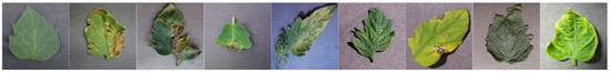
Figure 1.
Samples of tomato leaf images in our dataset includes 9 classes, from left to right: healthy leaf, bacterial spot, early blight, late blight, leaf mold, mosaic virus, septoria, target spot and yellow leaf.
The whole images of the database, with 9 classes, were divided into three parts: a training set, a validation set and an original testing set, as shown in Table 1. We first randomly selected 100 tomato leaf images from each disease category to create the original testing set. Then, training set was set up by 80% of the rest of the images. The other images were validation set samples. Resizing method was applied on these samples to ensure the size of each image was .

Table 1.
Number of samples for each disease category in dataset.
Then, we created two additional testing sets: the low-frequency leaf testing (LLT) set and the corruption-shift leaf testing (CLT) set. Samples of each additional set were generated by the original testing set images. The generation method of LLT set is presented in reference [31]. In CLT set, samples were produced by the benchmark of ImageNet-C [22].
The purpose of LLT set is to investigate the relationship between layer depth of the CNN and low-frequency identification bias, in order to design an efficient CNN architecture with reasonable layer depth. Discrete cosine transformation (DCT) was first applied onto samples of original testing set to achieve the frequency spectrums. Then, the frequency spectrums were divided into low-frequency components and high-frequency components by different manual thresholds. At last, the low-frequency reconstructed images and high-frequency reconstructed images were generated by equation:
where , are the elements of low-frequency and high-frequency reconstructed image and is the hyperparameter of threshold.
An example of the reconstructed images was shown in Figure 2.
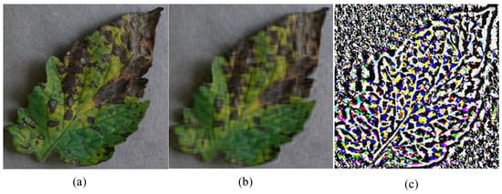
Figure 2.
Example of an original sample and the reconstructed samples: (a) An original early blight sample from the testing set; (b) The low-frequency reconstructed sample; (c) The high-frequency reconstructed sample. The hyperparameter of the threshold is 28.
To verify the generalization performance of each classification method for samples affected by corruption shifts, we created CLT set. It was composed of samples with 15 kinds of corruption shifts including Gaussian noise, shot noise, impulse noise, defocus blur, glass blur, motion blur, zoom blur, fog, frost, snow, brightness change, contrast transformation, elastic transformation, pixelation and JPEG, as shown in Figure 3.
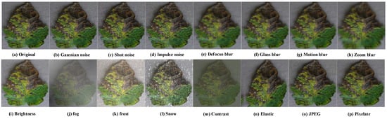
Figure 3.
Examples of corruption shifts. The samples are constructed by the benchmark of ImageNet-C, and the severity hyperparameter is set to 1.
2.2. Methods
Our proposed tomato disease classification method was based on an improved convolutional network. It was designed to take more focus on low-frequency components of the feature maps, and we named it MLFAnet. The whole architecture of the MLFAnet was shown in Figure 4a, and the detail of MLFA block was illustrated in Figure 4b.
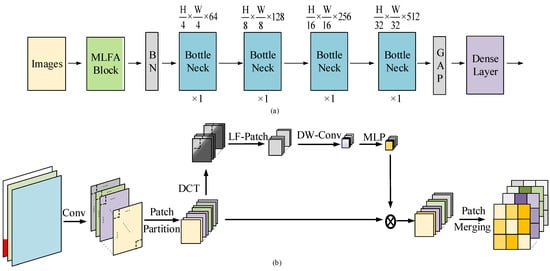
Figure 4.
(a) The architecture of a MLFAnet; (b) Illustration of MLFA block. The proposed block makes the architecture take more focus on low-frequency component of feature maps in order to improve the generalization of corruption shifts.
2.2.1. Generalization Gap and Frequency Components
In a conventional CNN classification task, the overall objective to train the model could be defined as:
where denotes the feature encoder with parameters of , denotes the classifier encoder which parameters are , is the softmax function, denotes the loss function and it is generally based on the cross-entropy method. are the optimal parameters learned by the CNN architecture.
Suppose the corruption shifts are caused by additive noise , the CNN model with the parameters may achieve a generalization gap which is affected by the factor and is calculated by the following equation:
To obtain the minimized value , Ganin et al. [32] demonstrate could be optimized by an extra loss function , then the total loss could be improved by the following equation:
where is domain confusion loss, is a hyper-parameter which is determined by . However, these references suppose the distribution of is known. Due to the randomness of in a generalization problem, it is difficult to optimize in spatial domain with the domain loss function , thus we transform the image and noise to the frequency domain by DCT [33], which can be defined as
where is a two-dimensional input signal and denotes the element at row and column in , is the height of input signal, the width of it is and is the frequency component corresponding to .
Another frequency-transform method is discrete Fourier transform (DFT). We applied DCT instead of DFT by the reason of DCT’s higher degree of spectral compaction. It was indicated in Figure 5. Lower frequency components were concentrated in four directions of DFT frequency spectrum, as shown in Figure 5b. Unlike DFT, lower frequency components are gathered in top left corner, as shown in Figure 5c.
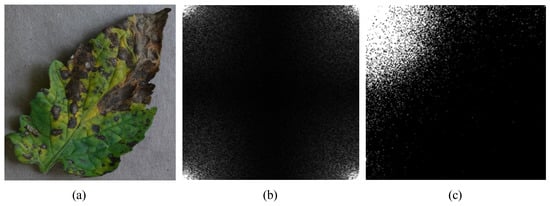
Figure 5.
Example of frequency-transform methods: (a) Original sample of early blight disease; (b) Frequency spectrum generated by discrete Fourier transform; (c) Frequency spectrum generated by DCT, where the lighter parts represent the lower frequency components on frequency domain.
The corruption shifts image are generally caused by pixel change. The change could be seen as a kind of noise image, which has the equal dimensions with the input image. We use and to represent the input image and image noise, in which denotes the channel number. Let , . Then, the frequency components of th channel in are , . As most of the image noise focus on the high-frequency components [34], there may exist the thresholding factors and which has the conditions for
where denotes the thresholding factor of generalization gap caused, which means the CNN model will occur the generalization gap problem if it focuses on the over-threshold frequency components. Thus, the method to improve the generalization gap can be regarded as making the model pay more attention to the frequency components under threshold .
2.2.2. Low-Frequency Attention for Domain Generalization
In the th convolutional layer of a CNN architecture, the feature map was calculated by the convolution kernels and features in th layer. To take a frequency point of view, it was created by filtering frequency components of features in th layer, and the convolution kernels were various of filters to fulfil high-pass, low-pass, brand-pass and band-stop.
To improve the performance of IID/OOD generalization gap, we increased the weight of feature maps which are created by low-pass filters, and the weight was learned by improved channel attention mechanism. The conventional channel attention algorithm could be defined as
where and are learned by the multi-layer perceptron (MLP) and dimensionality is reduced by for low complexity of the model. is the sigmoid function and is the weight vector of channel-wise to evaluate the importance of each channel.
Through Equation (7), we have
where is the frequency component of a feature tensor. Thus, from Equations (9) and (11), the weight vector of channel-wise can be defined as
Equation (12) shows that channel attention algorithm is a method to pay attention to the lowest frequency component of feature maps. It was proved experimentally in Section 3.2 that the method improved the IID/OOD generalization gap as well.
However, from Equation (8), we know that the lowest frequency component of a feature map is but not limited to the determining factors because all the frequency components under threshold may cause the generalization gap and should not be discarded. Thus, we calculated the weight by multiple low-frequency components instead of the lowest one. The low-frequency components tensor can be defined as
where and is a hyperparameter to adjust the threshold of significant low- frequency components.
2.2.3. Multiple Low-Frequency Attention Network Design
An overview of the proposed architecture MLFAnet was presented in Figure 4a. An input RGB image was first forward to the multiple low-frequency attention (MLFA) block, which was shown in Figure 4b. Several bottleneck blocks proposed by ResNet architecture [35] were applied afterwards, the output size of each bottleneck block was , , and , respectively. The output resolutions were forward to the dense layer which mixes the resulting output channels.
MLFA block was based on the proposed attention algorithm. As mentioned previously, the block was applied after an RGB input image. Feature map was derived with multiple filters in the CNN layer of the block, and it was split into patch, thus the feature dimension after patch partitioning was . Then the feature dimension was transformed to frequency component by DCT algorithm. The low-frequency tensor was derived by a manual threshold .
Depthwise convolution was applied on each channel of . The size of convolution kernel was . Then, the output vector was forward to MLP to obtain the weight vector . The updated feature dimension was calculated by and through the method of weighting with on the channel wise of . The final output tensor was generated by merging the patch in the updated feature dimension , and the size of is which was same as the feature map .
The number of bottleneck blocks in proposed MLFAnet is 1, 1, 1, 1, respectively. From accuracy performance perspective, deeper convolutional neural network was an effective method for classification and that was pointed out by [3,4,5]. To be specific, a deeper convolutional neural model could extract more abstract features from the deep layers [36], these abstract features are considered as high-frequency components and they improve the accuracy performance of the model [31]. Thus, various methods for tomato disease classification were based on a very deep-layer architecture and the efficiency is confirmed by the experiments [37]. We investigated the correlation between depth of model and impacts of corruption shifts sample generalization in tomato-disease classification, it had been found experimentally in Section 3.1 that a deeper model achieved a pool IID/OOD generalization gap though it improved the IID performance a little. Due to the reason above, the proposed MLFAnet deprecated stacking a large number of bottleneck blocks. The architecture is shown in Table 2, where hyperparameter denotes the kernel size of the convolution, denotes the stride, is the padding, represents the number of filters and P is the threshold of low-frequency patch.
Table 2.
Architecture of proposed MLFAnet.
2.3. Network Training and Evaluation
We carried out the experiments with an NVIDIA GeForce RTX 2080 GPU, an I7-9700k CPU and 16 GB of memory. The experimental environment was Python 3.7 (Guido van Rossum, Haarlem, Netherlands) and PyTorch 1.5.1 (Soumith Chintala, New York, NY, USA). The batch size, learning rate, number of training epochs and initial weights for all these networks were the same. The number of training epochs was set to 100, the batch size was 32 and learning rate was the exponential-decay learning rate.
3. Results
3.1. Relevance between Layer Depth and Low-Frequency Attention
To investigate the relationship between a number of network layers and low-frequency identification bias, we trained several different CNN architectures with similar ResNet and VGG backbones. The CNN architectures were ResNet-18, ResNet-34, ResNet-50, ResNet-101, ResNet-152, VGG-11, VGG-13, VGG-16 and VGG-19, respectively. Each of them has a diverse set of convolutional layers or bottleneck blocks. If the model takes more focus on low-frequency information, the accuracy performance on low-frequency reconstructed samples of the architecture will be better than others. Table 3 shows the comparison results of the models on the original testing set and LLT set. Ori. is the accuracy performance of samples in the testing-1 set. LFR indicates the accuracy results of low-frequency reconstructed samples in the LLT set, and the samples are reconstructed by frequency components under threshold . HFR represents the accuracy of high-frequency reconstructed samples. Gap denotes the generalization gap between Ori and LFR.
Table 3.
Accuracy result of original samples and reconstructed samples.
3.2. Accuracy Performance
We compared our method with the other conventional deep CNN architectures including ResNet-50 [38], DenseNet-121 [39], EffecientNet-b3 [40], ShuffleNet-v2 [41] and MobileNet-v3 [42]. Each of them was proved to be efficient in tomato disease classification. We trained the different CNN architectures on the same training set. Then, we tested and verified them by the original testing set and CLT set, respectively. Figure 6 shows the accuracy performance of each method on training and validation sets. Confusion matrices provided by different CNN architectures are shown in Figure 7.
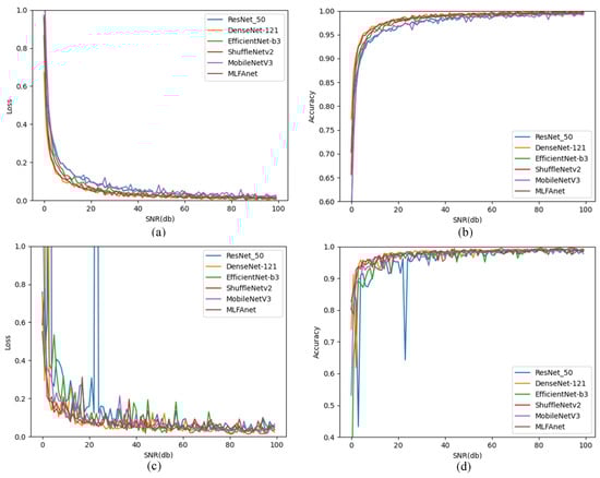
Figure 6.
Loss and accuracy curves on training and validation processes: (a) Training loss; (b) Training accuracy; (c) Validation loss; (d) Validation accuracy.
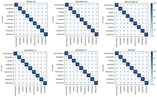
Figure 7.
Confusion matrixes for ResNet-50, DenseNet-121, EffecientNet-b3, ShuffleNet-v2, MobileNet-v3 and our proposed MLFAnet.
The accuracy results of CNN architectures on the original testing set and CLT set are shown in Table 4 and Table 5. Original represents the accuracy results on the original testing set. Gauss., Shot, Impluse, Defocus, Glass, Motion, Zoom, Bright, Fog, Frost, Snow, Contrast, Elastic, JPEG and Pixel represent the accuracy performance of different corruption factors on the CLT set.
Table 4.
Performance of CNN architecture under corruption shifts, including noises and blurs. The bold type represents the best classification performance of the architecture under a certain type of corruption.
Table 5.
Performance of CNN architecture under corruption shifts, including weathers and digital transforms. The bold type represents the best classification performance of the architecture under a certain type of corruption.
3.3. Experiments for Optimized Manual Thresholds
To investigate the optimized manual threshold of the MLFA block, we reconstructed the low-frequency sample as Equation (2). The size of the original image was , thus when the value of equaled 112, the sample was reconstructed by a quarter of the feature spectrum. The CNN architecture was modified by MLFAnet, which applied a conventional bottleneck block instead of an MLFA block. The accuracy results of low-frequency reconstructed samples with different thresholds were compared in Table 6.
Table 6.
Accuracy result of low-frequency reconstructed samples with different thresholds.
As shown in Table 6, the accuracy decreases as the manual threshold hyperparameter reduces, and it breaks down dramatically while is under 70. By observing Figure 5c, we conjectured the reason was that the low-frequency reconstructed sample traded off many low-frequency components which limited the model’s prediction precision. Thus, the hyperparameter of the MLFA block in Table 2 was set to 5, due to the patch size.
4. Discussion
The experiment results in Section 3.1 indicated that for tomato disease classification, both architectures with small-number layers (ResNet-18, VGG-11) and architectures with large-number layers (ResNet-152, VGG-19) could achieve high degrees of accuracy on original samples. As the high-frequency components decreased, the prediction accuracy of low-frequency reconstructed samples reduced more dramatically for the model with large-number layers. It indicated that a deeper model would be biased to neglect the low-frequency components. Low-frequency components are significant to the model’s generalization performance, this discovery could be applied to design a more efficient CNN architecture with reasonable layer depth.
In Section 3.2, the accuracy performances indicated that EffecientNet-b3 architecture, which achieved the highest accuracy rate (99.9%) in the original testing set, performed best on the IID tomato disease classification task. The other architectures, with accuracies of more than 99%, achieved excellent classification performance on IID testing samples as well. However, on corruption shifts samples of CLT set, the accuracy performances break down dramatically. It can be calculated in Table 4 and Table 5 that the average accuracy result of EffecientNet-b3 was 74.0%. The generalization gap was 25.9% (the difference value of 99% and 74.0%). The proposed MLFAnet achieved an average accuracy of 84.0% on corruption shifts samples, and the better generalization gap performance was 15.4%. To easily compare the generalization ability between different architectures, visual representations were shown in Figure 8.
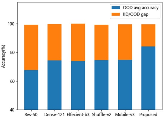
Figure 8.
Average accuracy on OOD samples and IID/OOD generalization gap of different CNN architecture.
Based on Figure 8, we could have the following observations. First, the average accuracy performance of our proposed method on corrupted samples classification was better than other conventional CNN architecture, as shown by the blue histogram. Second, the method had a better generalization performance because it achieved the smallest generalization gap, while the accuracy on original IID samples was almost identical to others, as shown by the orange histogram. It illustrates that the prediction model we proposed for tomato disease, which has a stronger generalization ability on corruption shifts samples, is a better fit than previous studies in practical application.
We further explored why our model achieved a strong generalization ability. Figure 9 showed the feature maps of the original sample and corruption shifts samples. The kinds of corruption were Gaussian noise and motion blur. The features were the first convolution layer outputs of conventional ResNet-50 architecture and the proposed MLFAnet architecture. It observed that feature maps extracted by ResNet-50 changed sharply as the samples were corrupted by Gaussian noise and motion blur. On the contrary, the diversity among the feature maps was less under the proposed MLFAnet architecture. The example demonstrated that the feature extractor of MLFAnet was more robust on corruption shifts. It helped to improve the accuracy performance of the classifier on corruption shifts samples.
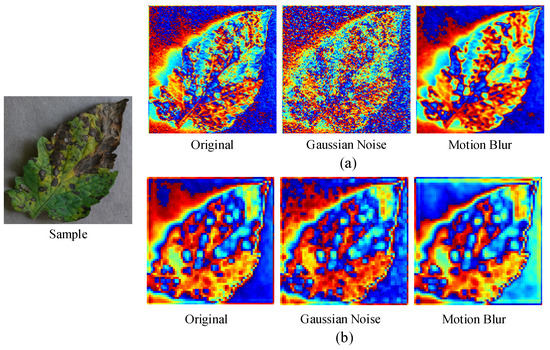
Figure 9.
Feature maps of the original sample and corruption shifts samples: (a) 1st convolution layer output of ResNet-50; (b) 1st convolution layer output of proposed MLFAnet. Gaussian-noise corruption and motion-blur corruption are shown as illustrations.
Comprehensive experiments showed that the MLFAnet performed well on benchmarks of corruption shift generalization. Furthermore, the prediction of noise and blur corruption shifts samples, in particular, had a dramatically improved. It indicated that the MLFAnet may provide support for the real-world diagnosis of tomato disease, i.e., it can diagnose the disease accurately from a blur leaf image which is captured by a shaking camera or a moving device. However, when the leaf images are affected by weather corruption and contrast transformation, the classification performance of MLFAnet is not outstanding. It shows that accurate diagnosis of MLFAnet is limited in complex weather conditions.
5. Conclusions
In this work, we investigated the OOD generalization of CNN architectures and proposed an efficient classification method for tomato disease. The method with a better capacity of generalization could diagnose tomato disease more accurately from corruption shifts images while retaining the satisfying classification performance of original images.
From our study and simulation results, we may obtain the following conclusions: (1) CNN may degrade the generalization ability while focusing on high-frequency components. (2) For a basic classification task, such as tomato disease with nine categories, the accuracy precision on IID samples of a shallow CNN architecture is similar to that of DCNN models. However, shallow-layer CNN architecture has a better OOD generalization performance. (3) Results verify the hypothesis that attention mechanisms are capable of improving the generalization performance of deep CNN models. For these reasons, an improved attention algorithm was proposed by calculating the weight of feature maps with multiple low-frequency components, and it has been demonstrated the effectiveness of corruption shifts generalization. Moreover, we provided an efficient CNN method named MLFAnet to improve the generalization on the diagnosis of tomato disease. An interesting question to make further progress would be verifying the effectiveness of MLFAnet on other fruits or vegetables. Though we consider our proposed method is based on a general CNN system, it can be applied to most of the image classification tasks with a high probability. However, extra work and experiments should be designed to prove it for further study.
Our work on corruption shifts sample generalization could scale to the real-world problem, which is left for future investigation.
Author Contributions
For Conceptualization, D.L. and Z.Y.; method design, D.L.; code, D.L.; validation, D.L., Y.Z. and Z.Y.; formal analysis, D.L.; investigation, D.L. and W.Z.; resources, Y.Z.; data collection, J.L.; writing—original draft preparation, D.L.; writing—review and editing, D.L.; visualization, D.L.; supervision, Y.Z. and Z.Y.; project administration, D.L.; funding acquisition, Z.Y. All authors have read and agreed to the published version of the manuscript.
Funding
The research was supported by the National Natural Science Foundation of China (grant number 62071143).
Institutional Review Board Statement
Not applicable.
Data Availability Statement
The data presented in this study are available on request from the corresponding author. The data are not publicly available due to the privacy.
Conflicts of Interest
The authors declare no conflict of interest.
References
- Ropelewska, E.; Sabanci, K.; Aslan, M.F. Authentication of tomato (Solanum lycopersicum L.) cultivars using discriminative models based on texture parameters of flesh and skin images. Eur. Food Res. Technol. 2022, 248, 1959–1976. [Google Scholar] [CrossRef]
- Ropelewska, E.; Slavova, V.; Sabanci, K.; Aslan, M.F.; Masheva, V.; Petkova, M. Differentiation of Yeast-Inoculated and Uninoculated Tomatoes Using Fluorescence Spectroscopy Combined with Machine Learning. Agriculture 2022, 12, 1887. [Google Scholar] [CrossRef]
- Borhani, Y.; Khoramdel, J.; Najafi, E. A deep learning based approach for automated plant disease classification using vision transformer. Sci. Rep. 2022, 12, 11554. [Google Scholar] [CrossRef] [PubMed]
- Zhao, Y.; Sun, C.; Xu, X.; Chen, J. RIC-Net: A plant disease classification model based on the fusion of Inception and residual structure and embedded attention mechanism. Comput. Electron. Agric. 2022, 193, 106644. [Google Scholar] [CrossRef]
- Shruthi, U.; Nagaveni, V.; Arvind, C.S.; Sunil, G.L. Tomato Plant Disease Classification Using Deep Learning Architectures: A Review. In Proceedings of Second International Conference on Advances in Computer Engineering and Communication Systems: ICACECS 2021; Springer Nature: Singapore, 2022; pp. 153–169. [Google Scholar]
- Tm, P.; Pranathi, A.; SaiAshritha, K.; Chittaragi, N.B.; Koolagudi, S.G. Tomato leaf disease detection using convolutional neural networks. In Proceedings of the 2018 Eleventh International Conference on Contemporary Computing (IC3), Noida, India, 2–4 August 2018; IEEE: Piscataway, NJ, USA, 2018; pp. 1–5. [Google Scholar]
- Tan, L.; Lu, J.; Jiang, H. Tomato leaf diseases classification based on leaf images: A comparison between classical machine learning and deep learning methods. AgriEngineering 2021, 3, 542–558. [Google Scholar] [CrossRef]
- Rangarajan, A.K.; Purushothaman, R.; Ramesh, A. Tomato crop disease classification using pre-trained deep learning algorithm. Procedia Comput. Sci. 2018, 133, 1040–1047. [Google Scholar] [CrossRef]
- Karthik, R.; Hariharan, M.; Anand, S.; Mathikshara, P.; Johnson, A.; Menaka, R. Attention embedded residual CNN for disease detection in tomato leaves. Appl. Soft Comput. 2020, 86, 105933. [Google Scholar]
- Bhujel, A.; Kim, N.E.; Arulmozhi, E.; Basak, J.K.; Kim, H.T. A lightweight Attention-based convolutional neural networks for tomato leaf disease classification. Agriculture 2022, 12, 228. [Google Scholar] [CrossRef]
- Kamal, K.C.; Yin, Z.; Wu, M.; Wu, Z. Depthwise separable convolution architectures for plant disease classification. Comput. Electron. Agric. 2019, 165, 104948. [Google Scholar]
- Qiao, F.; Zhao, L.; Peng, X. Learning to learn single domain generalization. In Proceedings of the IEEE/CVF Conference on Computer Vision and Pattern Recognition, Seattle, WA, USA, 13–19 June 2020; pp. 12556–12565. [Google Scholar]
- Zhang, C.; Zhang, M.; Zhang, S.; Jin, D.; Zhou, Q.; Cai, Z.; Zhao, H.; Liu, X.; Liu, Z. Delving deep into the generalization of vision transformers under distribution shifts. In Proceedings of the IEEE/CVF Conference on Computer Vision and Pattern Recognition, Seattle, WA, USA, 18–24 June 2022; pp. 7277–7286. [Google Scholar]
- Kamal, K.C.; Yin, Z.; Li, D.; Wu, Z. Impacts of Background Removal on Convolutional Neural Networks for Plant Disease Classification In-Situ. Agriculture 2021, 11, 827. [Google Scholar]
- Shen, Y.; Zheng, L.; Shu, M.; Li, W.; Goldstein, T.; Lin, M. Gradient-free adversarial training against image corruption for learning-based steering. Adv. Neural Inf. Process. Syst. 2021, 34, 26250–26263. [Google Scholar]
- Brendel, W.; Bethge, M. Approximating CNNs with Bag-of-local-Features models works surprisingly well on ImageNet. In Proceedings of the International Conference on Learning Representations, Vancouver, BC, Canada, 30 April–3 May 2018. [Google Scholar]
- Peng, X.; Bai, Q.; Xia, X.; Huang, Z.; Saenko, K.; Wang, B. Moment matching for multi-source domain adaptation. In Proceedings of the IEEE/CVF International Conference on Computer Vision, Seoul, Republic of Korea, 27 October–2 November 2019; pp. 1406–1415. [Google Scholar]
- Jiang, Y.; Krishnan, D.; Mobahi, H.; Bengio, S. Predicting the Generalization Gap in Deep Networks with Margin Distribu-tions. In Proceedings of the International Conference on Learning Representations, Vancouver, BC, Canada, 30 April–3 May 2018. [Google Scholar]
- Morbekar, A.; Parihar, A.; Jadhav, R. Crop disease detection using YOLO. In Proceedings of the 2020 International Conference for Emerging Technology (INCET), Belgaum, India, 5–7 June 2020; IEEE: Piscataway, NJ, USA, 2020; pp. 1–5. [Google Scholar]
- Mathew, M.P.; Mahesh, T.Y. Leaf-based disease detection in bell pepper plant using YOLO v5. Signal Image Video Process. 2022, 16, 841–847. [Google Scholar] [CrossRef]
- Liu, J.; Wang, X. Tomato diseases and pests detection based on improved Yolo V3 convolutional neural network. Front. Plant Sci. 2020, 11, 898. [Google Scholar] [CrossRef] [PubMed]
- Hendrycks, D.; Dietterich, T. Benchmarking Neural Network Robustness to Common Corruptions and Perturbations. In Proceedings of the International Conference on Learning Representations, Vancouver, BC, Canada, 30 April–3 May 2018. [Google Scholar]
- Wagle, S.A.; Sampe, J.; Mohammad, F.; Ali, S.H. Effect of Data Augmentation in the Classification and Validation of Tomato Plant Disease with Deep Learning Methods. Traitement Du Signal 2021, 38, 1657–1670. [Google Scholar] [CrossRef]
- Nazki, H.; Lee, J.; Yoon, S.; Park, D.S. Synthetic data augmentation for plant disease image generation using GAN. In Proceedings of the Korea Contents Association Conference, Seoul, Republic of Korea, 26–28 June 2018; pp. 459–460. [Google Scholar]
- Yilma, G.; Gedamu, K.; Assefa, M.; Oluwasanmi, A.; Qin, Z. Generation and Transformation Invariant Learning for Tomato Disease Classification. In Proceedings of the 2021 IEEE 2nd International Conference on Pattern Recognition and Machine Learning (PRML), Chengdu, China, 16–18 July 2021; IEEE: Piscataway, NJ, USA, 2021; pp. 121–128. [Google Scholar]
- Nazki, H.; Yoon, S.; Fuentes, A.; Park, D.S. Unsupervised image translation using adversarial networks for improved plant disease recognition. Comput. Electron. Agric. 2020, 168, 105117. [Google Scholar] [CrossRef]
- Bi, L.; Hu, G. Improving image-based plant disease classification with generative adversarial network under limited training set. Front. Plant Sci. 2020, 11, 583438. [Google Scholar] [CrossRef]
- You, H.; Lu, Y.; Tang, H. Plant Disease Classification and Adversarial Attack Using SimAM-EfficientNet and GP-MI-FGSM. Sustainability 2023, 15, 1233. [Google Scholar] [CrossRef]
- Tsipras, D.; Santurkar, S.; Engstrom, L.; Turner, A.; Madry, A. Robustness May Be at Odds with Accuracy. In Proceedings of the International Conference on Learning Representations, Vancouver, BC, Canada, 30 April–3 May 2018. [Google Scholar]
- Hughes, D.; Salathé, M. An open access repository of images on plant health to enable the development of mobile disease diagnostics. arXiv 2015, arXiv:1511.08060. [Google Scholar]
- Wang, H.; Wu, X.; Huang, Z.; Xing, E.P. High-frequency component helps explain the generalization of convolutional neural networks. In Proceedings of the IEEE/CVF Conference on Computer Vision and Pattern Recognition, Virtually, 14–19 June 2020; pp. 8684–8694. [Google Scholar]
- Ganin, Y.; Ustinova, E.; Ajakan, H.; Germain, P.; Larochelle, H.; Laviolette, F.; Marchand, M.; Lempitsky, V. Domain-adversarial training of neural networks. J. Mach. Learn. Res. 2016, 17, 1–35. [Google Scholar]
- Ahmed, N.; Natarajan, T.; Rao, K.R. Discrete cosine transform. IEEE Trans. Comput. 1974, 100, 90–93. [Google Scholar] [CrossRef]
- Li, Q.; Shen, L.; Guo, S.; Lai, Z. Wavelet integrated CNNs for noise-robust image classification. In Proceedings of the IEEE/CVF Conference on Computer Vision and Pattern Recognition, New Orleans, LA, USA, 13–19 June 2020; pp. 7245–7254. [Google Scholar]
- He, K.; Zhang, X.; Ren, S.; Sun, J. Deep residual learning for image recognition. In Proceedings of the IEEE Conference on Computer Vision and Pattern Recognition, Las Vegas, NV, USA, 27–30 June 2016; pp. 770–778. [Google Scholar]
- Yosinski, J.; Clune, J.; Bengio, Y.; Lipson, H. How transferable are features in deep neural networks? Adv. Neural Inf. Process. Syst. 2014, 27, 3320–3328. [Google Scholar]
- Pattnaik, G.; Shrivastava, V.K.; Parvathi, K. Transfer learning-based framework for classification of pest in tomato plants. Appl. Artif. Intell. 2020, 34, 981–993. [Google Scholar] [CrossRef]
- Kumar, S.; Pal, S.; Singh, V.P.; Jaiswal, P. Performance evaluation of ResNet model for classification of tomato plant disease. Epidemiol. Methods 2023, 12, 20210044. [Google Scholar] [CrossRef]
- Verma, R.; Singh, V. Leaf Disease Identification Using DenseNet. In Proceedings of the Artificial Intelligence and Speech Technology: Third International Conference, AIST 2021, Delhi, India, 12–13 November 2021; Revised Selected Papers. Springer International Publishing: Cham, Switzerland, 2022; pp. 500–511. [Google Scholar]
- Malik, O.A.; Ismail, N.; Hussein, B.R.; Yahya, U. Automated Real-Time Identification of Medicinal Plants Species in Natural Environment Using Deep Learning Models—A Case Study from Borneo Region. Plants 2022, 11, 1952. [Google Scholar] [CrossRef]
- Jiang, J.; Liu, H.; Zhao, C.; He, C.; Ma, J.; Cheng, T.; Zhu, Y.; Cao, W.; Yao, X. Evaluation of Diverse Convolutional Neural Networks and Training Strategies for Wheat Leaf Disease Identification with Field-Acquired Photographs. Remote Sens. 2022, 14, 3446. [Google Scholar] [CrossRef]
- Qiaoli, Z.; Li, M.A.; Liying, C.A.O.; Helong, Y.U. Identification of tomato leaf diseases based on improved lightweight convolutional neural networks MobileNetV3. Smart Agric. 2022, 4, 47. [Google Scholar]
Disclaimer/Publisher’s Note: The statements, opinions and data contained in all publications are solely those of the individual author(s) and contributor(s) and not of MDPI and/or the editor(s). MDPI and/or the editor(s) disclaim responsibility for any injury to people or property resulting from any ideas, methods, instructions or products referred to in the content. |
© 2023 by the authors. Licensee MDPI, Basel, Switzerland. This article is an open access article distributed under the terms and conditions of the Creative Commons Attribution (CC BY) license (https://creativecommons.org/licenses/by/4.0/).