
Assessing the Within-Field Heterogeneity Using Rapid-Eye NDVI Time Series Data


Abstract
1. Introduction
2. Materials and Methods
3. Results
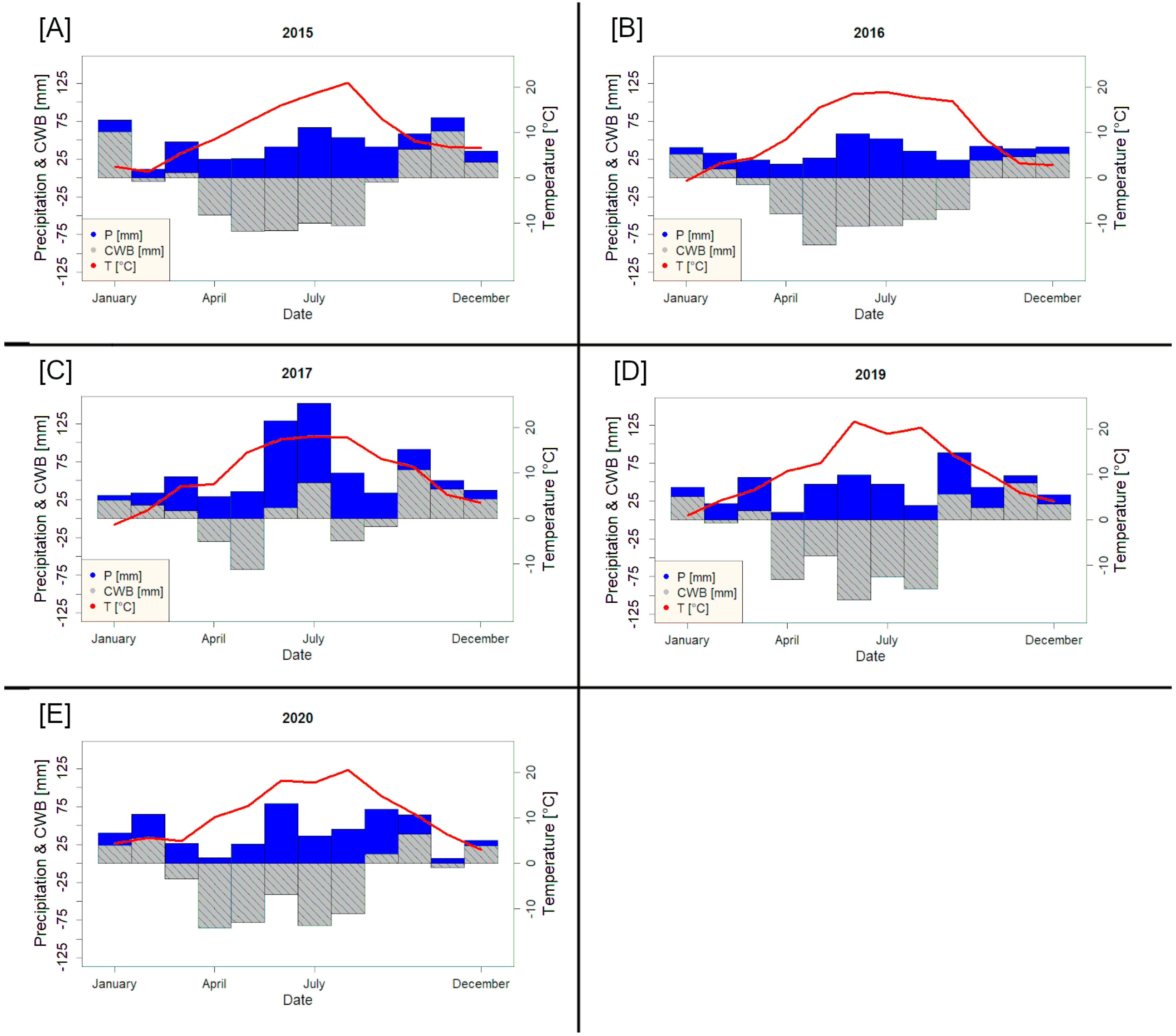
3.1. Climate
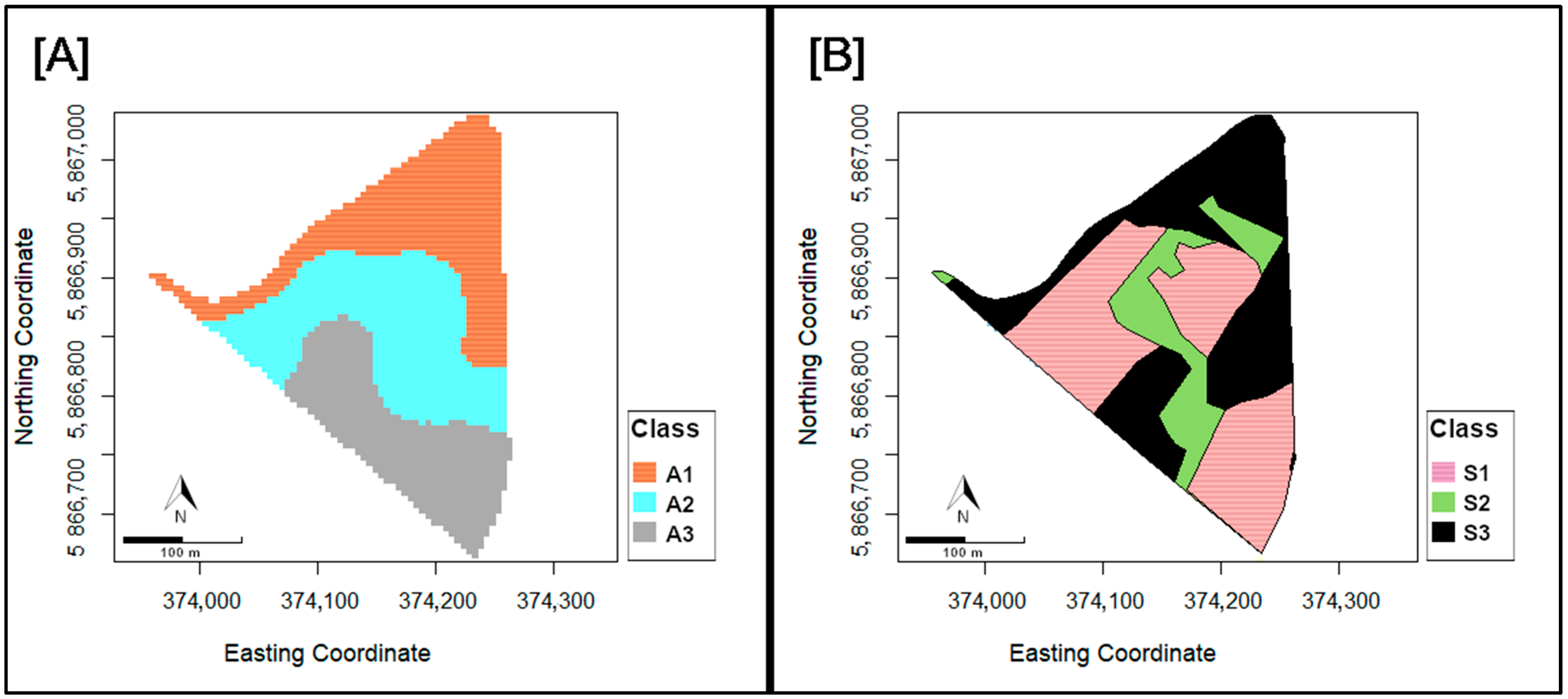
3.2. Variation of the NDVI in Altitude and Soil Classes
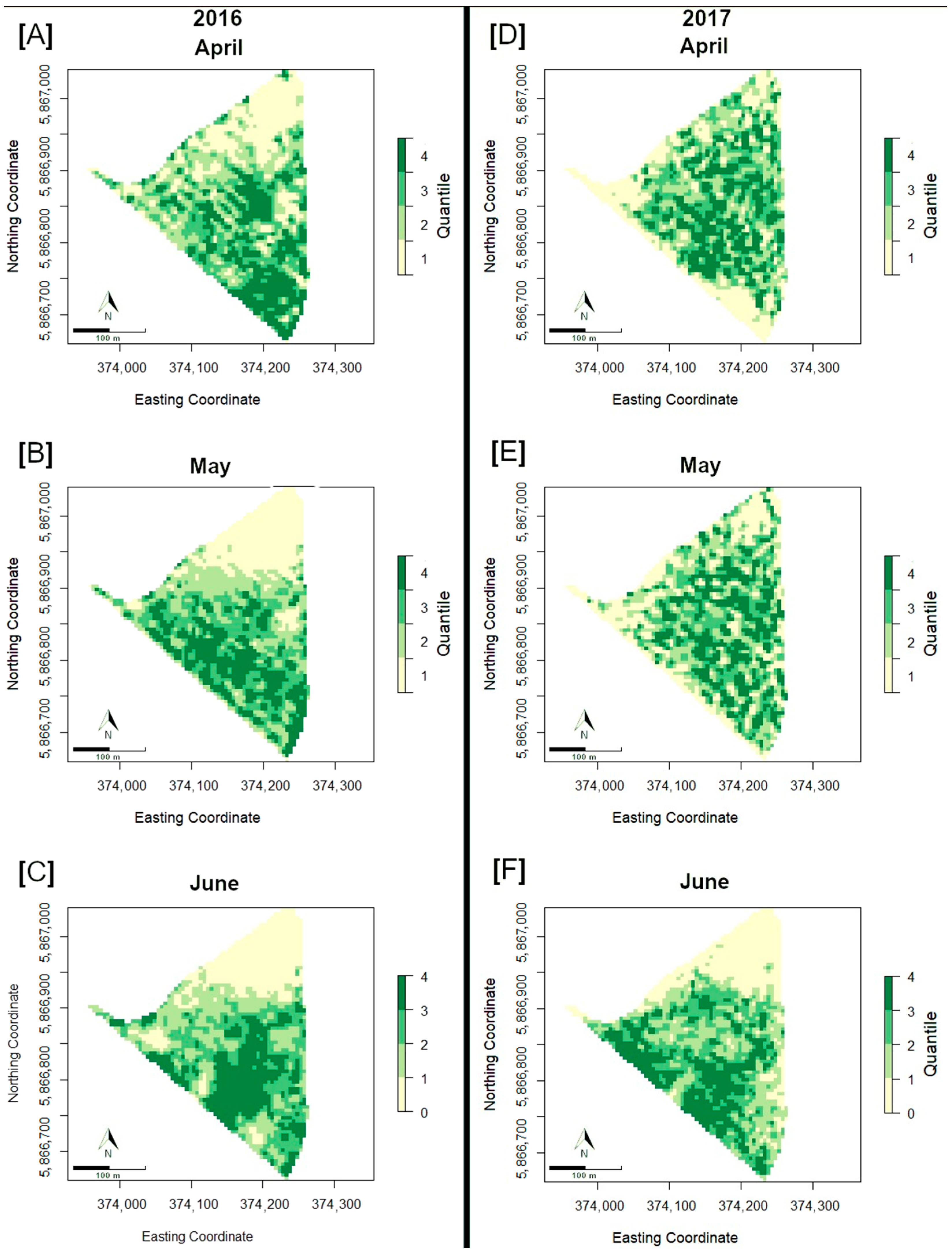
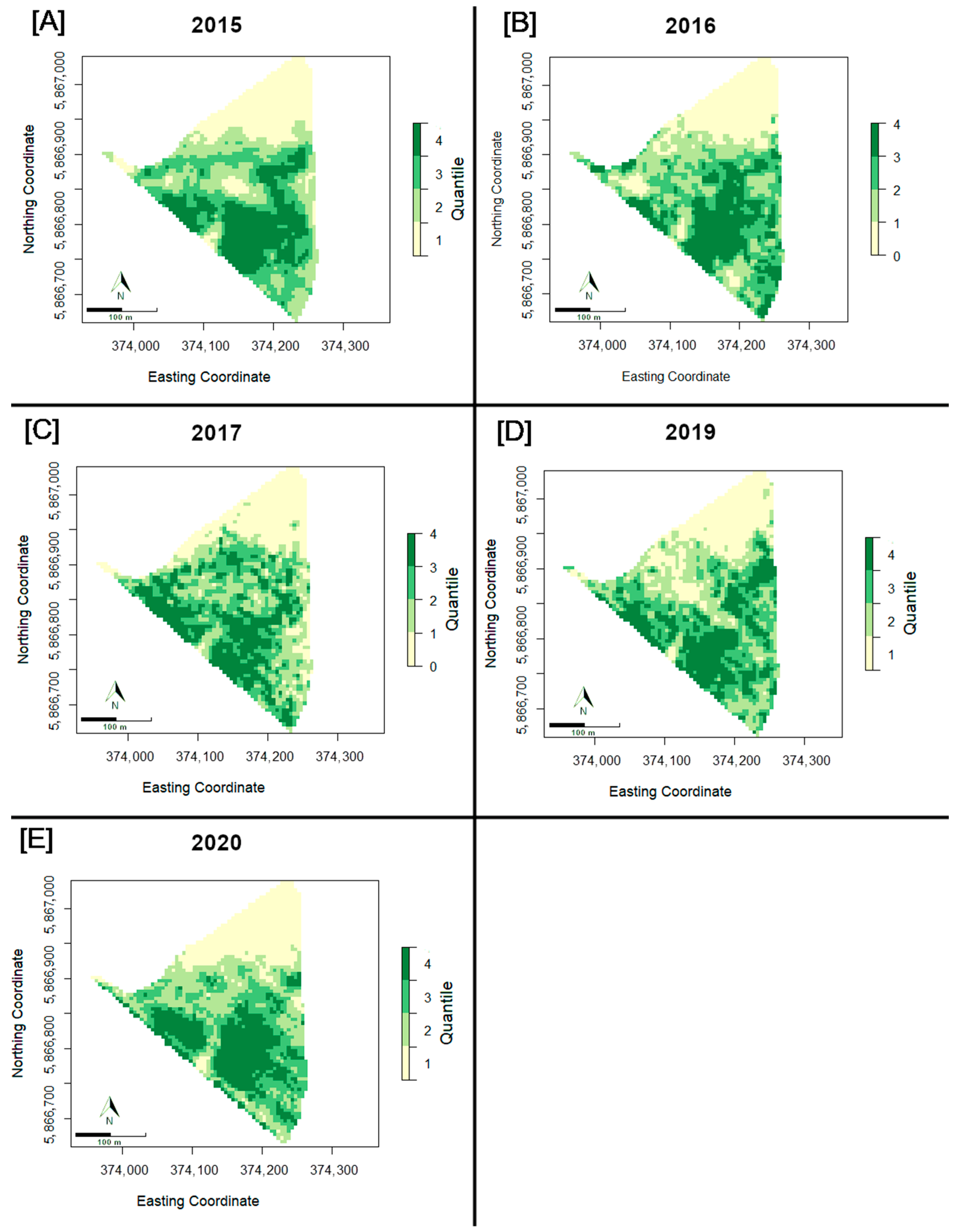
3.3. Spatial Distribution of NDVI over Time
4. Discussion
4.1. Spatial Distribution of NDVI
4.2. Influence of Weather Conditions on Spatial Patterns of NDVI at Field Scale
5. Conclusions
Supplementary Materials
Author Contributions
Funding
Institutional Review Board Statement
Data Availability Statement
Acknowledgments
Conflicts of Interest
References
- Yuzugullu, O.; Lorenz, F.; Fröhlich, P.; Liebisch, F. Understanding Fields by Remote Sensing: Soil Zoning and Property Mapping. Remote Sens. 2020, 12, 1116. [Google Scholar] [CrossRef]
- Kravchenko, A.N.; Thelen, K.D.; Bullock, D.G.; Miller, N.R. Relationship among Crop Grain Yield, Topography, and Soil Electrical Conductivity Studied with Cross-Correlograms. Agron. J. 2003, 95, 1132–1139. [Google Scholar] [CrossRef]
- Huang, X.; Wang, L.; Yang, L.; Kravchenko, A.N. Management Effects on Relationships of Crop Yields with Topography Represented by Wetness Index and Precipitation. Agron. J. 2008, 100, 1463–1471. [Google Scholar] [CrossRef]
- Thelemann, R.; Johnson, G.; Sheaffer, C.; Banerjee, S.; Cai, H.; Wyse, D. The Effect of Landscape Position on Biomass Crop Yield. Agron. J. 2010, 102, 513–522. [Google Scholar] [CrossRef]
- Kumhálová, J.; Kumhála, F.; Kroulík, M.; Matějková, Š. The Impact of Topography on Soil Properties and Yield and the Effects of Weather Conditions. Precis. Agric. 2011, 12, 813–830. [Google Scholar] [CrossRef]
- Xue, W.; Huang, L.; Yu, F.-H. Spatial Heterogeneity in Soil Particle Size: Does It Affect the Yield of Plant Communities with Different Species Richness? J. Plant Ecol. 2016, 9, 608–615. [Google Scholar] [CrossRef]
- Beuschel, R.; Piepho, H.-P.; Joergensen, R.G.; Wachendorf, C. Similar Spatial Patterns of Soil Quality Indicators in Three Poplar-Based Silvo-Arable Alley Cropping Systems in Germany. Biol. Fertil. Soils 2019, 55, 1–14. [Google Scholar] [CrossRef]
- Sahoo, R.; Ray, S.S.; Manjunath, K. Hyperspectral Remote Sensing of Agriculture. Curr. Sci. 2015, 108, 848–859. [Google Scholar]
- Kumhálová, J.; Novák, P.; Madaras, M. Monitoring Oats and Winter Wheat Within-Field Spatial Variability by Satellite Images. Sci. Agric. Bohem. 2018, 49, 127–135. [Google Scholar] [CrossRef]
- Jiang, P.; Thelen, K.D. Effect of Soil and Topographic Properties on Crop Yield in a North-Central Corn–Soybean Cropping System. Agron. J. 2004, 96, 252–258. [Google Scholar] [CrossRef]
- Stadler, A.; Rudolph, S.; Kupisch, M.; Langensiepen, M.; van der Kruk, J.; Ewert, F. Quantifying the Effects of Soil Variability on Crop Growth Using Apparent Soil Electrical Conductivity Measurements. Eur. J. Agron. 2015, 64, 8–20. [Google Scholar] [CrossRef]
- He, D.; Wang, E. On the Relation between Soil Water Holding Capacity and Dryland Crop Productivity. Geoderma 2019, 353, 11–24. [Google Scholar] [CrossRef]
- Deutscher Wetterdienst (DWD). Klimareport Brandenburg. Fakten Bis Zur Gegenwart—Erwartungen Für Die Zukunft 2020; Deutscher Wetterdienst (DWD): Offenbach am Main, Germany, 2019. [Google Scholar]
- Deutscher Wetterdienst (DWD). Mean Precipitation Neuruppin 1991–2020; Deutscher Wetterdienst (DWD): Offenbach am Main, Germany. Available online: https://opendata.dwd.de/climate_environment/CDC/observations_germany and https://opendata.dwd.de/climate_environment/CDC/grids_germany/ (accessed on 8 February 2023).
- Deutscher Wetterdienst (DWD). Mean Temperature Neuruppin 1991–2020; Deutscher Wetterdienst (DWD): Offenbach am Main, Germany. Available online: https://opendata.dwd.de/climate_environment/CDC/observations_germany and https://opendata.dwd.de/climate_environment/CDC/grids_germany/ (accessed on 8 February 2023).
- Habib-ur-Rahman, M.; Raza, A.; Ahrends, H.E.; Hüging, H.; Gaiser, T. Impact of In-Field Soil Heterogeneity on Biomass and Yield of Winter Triticale in an Intensively Cropped Hummocky Landscape under Temperate Climate Conditions. Precis. Agric. 2022, 23, 912–938. [Google Scholar] [CrossRef]
- Kopp, D. Die Böden Des Nordostdeutschen Tieflands Und Ihre Zusammenwirkung Mit Relief, Klima Und Vegetation; BGR, Bundesanstalt für Geowissenschaften und Rohstoffe: Berlin, Germany, 2003. [Google Scholar]
- IUSS Working Group WRB. World Reference Base for Soil Resources 2006; World Soil Resources Reports; FAO: Rome, Italy, 2006. [Google Scholar]
- Munsell Color (Firm). Munsell Soil Color Charts: With Genuine Munsell Color Chips; 2009 year revised; Munsell Color: Grand Rapids, MI, USA, 2010. [Google Scholar]
- Baxter, S. Guidelines for Soil Description. Rome: Food and Agriculture Organization of the United Nations. (2006), pp. 108, US$40.00. ISBN 92-5-1055-21-1. Exp. Agric. 2007, 43, 263–264. [Google Scholar] [CrossRef]
- Huang, J.; Hartemink, A.E. Soil and Environmental Issues in Sandy Soils. Earth-Sci. Rev. 2020, 208, 103295. [Google Scholar] [CrossRef]
- Planet Labs PBC. Planet Labs Planet Imagery Product Specifications; Planet Labs PBC: San Francisco, CA, USA, 2022. [Google Scholar]
- Rouse, J.W.; Haas, R.H.; Schell, J.A.; Deering, D.W. Monitoring Vegetation Systems in the Great Plains with ERTS. NASA Spec. Publ. 1974, 351, 309. [Google Scholar]
- Tucker, C.J. Red and Photographic Infrared Linear Combinations for Monitoring Vegetation. Remote Sens. Environ. 1979, 8, 127–150. [Google Scholar] [CrossRef]
- R Core Team. R: A Language and Environment for Statistical Computing; R Foundation for Statistical Computing: Vienna, Austria, 2021. [Google Scholar]
- Hijmans, R.J. Raster: Geographic Data Analysis and Modeling. 2022. Available online: http://CRAN.R-project.org/package=raster (accessed on 3 May 2023).
- Kruskal, W.H.; Wallis, W.A. Use of Ranks in One-Criterion Variance Analysis. J. Am. Stat. Assoc. 1952, 47, 583–621. [Google Scholar] [CrossRef]
- Wilcoxon, F. Individual Comparisons by Ranking Methods. Biom. Bull. 1945, 1, 80–83. [Google Scholar] [CrossRef]
- Benjamini, Y.; Hochberg, Y. Controlling the False Discovery Rate: A Practical and Powerful Approach to Multiple Testing. J. R. Stat. Soc. Ser. B (Methodol.) 1995, 57, 289–300. [Google Scholar] [CrossRef]
- Mann, H.B. Nonparametric Tests Against Trend. Econometrica 1945, 13, 245–259. [Google Scholar] [CrossRef]
- McLeod, A.I. Kendall: Kendall Rank Correlation and Mann-Kendall Trend Test. Am. J. Clim. Chang. 2018, 7, 1. [Google Scholar]
- Kumar, S.; Machiwal, D.; Dayal, D. Spatial Modelling of Rainfall Trends Using Satellite Datasets and Geographic Information System. Hydrol. Sci. J. 2017, 62, 1636–1653. [Google Scholar] [CrossRef]
- Hipel, K.W.; McLeod, A.I. Time Series Modelling of Water Resources and Environmental Systems. In Developments in Water Science, 1st ed.; Elsevier: Amsterdam, The Netherlands, 1974; Volume 45, Available online: https://www.elsevier.com/books/time-series-modelling-of-water-resources-and-environmental-systems/hipel/978-0-444-89270-6 (accessed on 2 April 2023).
- Rakovec, O.; Samaniego, L.; Hari, V.; Markonis, Y.; Moravec, V.; Thober, S.; Hanel, M.; Kumar, R. The 2018–2020 Multi-Year Drought Sets a New Benchmark in Europe. Earth’s Future 2022, 10, e2021EF002394. [Google Scholar] [CrossRef]
- Boken, V.K.; Shaykewich, C.F. Improving an Operational Wheat Yield Model Using Phenological Phase-Based Normalized Difference Vegetation Index. Int. J. Remote Sens. 2002, 23, 4155–4168. [Google Scholar] [CrossRef]
- Wall, L.; Larocque, D.; Léger, P. The Early Explanatory Power of NDVI in Crop Yield Modelling. Int. J. Remote Sens. 2008, 29, 2211–2225. [Google Scholar] [CrossRef]
- Mkhabela, M.S.; Bullock, P.; Raj, S.; Wang, S.; Yang, Y. Crop Yield Forecasting on the Canadian Prairies Using MODIS NDVI Data. Agric. For. Meteorol. 2011, 151, 385–393. [Google Scholar] [CrossRef]
- Stoy, P.C.; Khan, A.M.; Wipf, A.; Silverman, N.; Powell, S.L. The Spatial Variability of NDVI within a Wheat Field: Information Content and Implications for Yield and Grain Protein Monitoring. PLoS ONE 2022, 17, e0265243. [Google Scholar] [CrossRef]
- Fry, J.E.; Guber, A.K. Temporal Stability of Field-Scale Patterns in Soil Water Content across Topographically Diverse Agricultural Landscapes. J. Hydrol. 2020, 580, 124260. [Google Scholar] [CrossRef]
- McGoverin, C.M.; Snyders, F.; Muller, N.; Botes, W.; Fox, G.; Manley, M. A Review of Triticale Uses and the Effect of Growth Environment on Grain Quality. J. Sci. Food Agric. 2011, 91, 1155–1165. [Google Scholar] [CrossRef]
- Prabhakara, K.; Hively, W.D.; McCarty, G.W. Evaluating the Relationship between Biomass, Percent Groundcover and Remote Sensing Indices across Six Winter Cover Crop Fields in Maryland, United States. Int. J. Appl. Earth Obs. Geoinf. 2015, 39, 88–102. [Google Scholar] [CrossRef]
- Diacono, M.; Castrignanò, A.; Troccoli, A.; De Benedetto, D.; Basso, B.; Rubino, P. Spatial and Temporal Variability of Wheat Grain Yield and Quality in a Mediterranean Environment: A Multivariate Geostatistical Approach. Field Crops Res. 2012, 131, 49–62. [Google Scholar] [CrossRef]
- Vicente-Serrano, S.M.; Gouveia, C.; Camarero, J.J.; Beguería, S.; Trigo, R.; López-Moreno, J.I.; Azorín-Molina, C.; Pasho, E.; Lorenzo-Lacruz, J.; Revuelto, J.; et al. Response of Vegetation to Drought Time-Scales across Global Land Biomes. Proc. Natl. Acad. Sci. USA 2013, 110, 52–57. [Google Scholar] [CrossRef] [PubMed]
- Peled, E.; Dutra, E.; Viterbo, P.; Angert, A. Technical Note: Comparing and Ranking Soil Drought Indices Performance over Europe, through Remote-Sensing of Vegetation. Hydrol. Earth Syst. Sci. 2010, 14, 271–277. [Google Scholar] [CrossRef]
- Piedallu, C.; Chéret, V.; Denux, J.P.; Perez, V.; Azcona, J.S.; Seynave, I.; Gégout, J.C. Soil and Climate Differently Impact NDVI Patterns According to the Season and the Stand Type. Sci. Total Environ. 2019, 651, 2874–2885. [Google Scholar] [CrossRef] [PubMed]


| Growing Season | Specie | Cultivar |
|---|---|---|
| 2014/15 | Winter triticale (×Triticosecale) | Talentro |
| 2015/16 | Winter triticale (×Triticosecale) | Lombardo |
| 2016/17 | Winter rye (Secale cereale) | KWS Bono |
| 2017/18 | Summer oat (Avena sativa) | Poseidon |
| 2018/19 | Winter barley (Hordeum vulgare) | Anja |
| 2019/20 | Winter triticale (×Triticosecale) | Lombardo |
| Date | Satellite Constellation |
|---|---|
| 15 April 2015 | RapidEye |
| 24 May 2015 | RapidEye |
| 12 June 2015 | RapidEye |
| 23 April 2016 | RapidEye |
| 11 May 2016 | RapidEye |
| 08 June 2016 | RapidEye |
| 22 April 2017 | RapidEye |
| 19 May 2017 | RapidEye |
| 11 June 2017 | RapidEye |
| 23 April 2019 | RapidEye |
| 05 June 2019 | RapidEye |
| 21 April 2020 | PlanetScope |
| 21 May 2020 | PlanetScope |
| 15 June 2020 | PlanetScope |
| Class | Definition | Numbers of Grid Cell [n] | Area [m2] |
|---|---|---|---|
| S1 | Loamy layer at <60 cm depth | 951 | 23.775 |
| S2 | Loamy layer at 60–100 cm depth | 351 | 8.775 |
| S3 | No loamy layer | 879 | 21.975 |
| A1 | <53.5 m a.s.l. | 752 | 18.800 |
| A2 | 53.5–55.37 m a.s.l. | 804 | 20.100 |
| A3 | >55.37 m a.s.l. | 625 | 15.625 |
| Class | S1 | S2 | S3 |
|---|---|---|---|
| A1 | 97 | 100 | 554 |
| A2 | 461 | 171 | 174 |
| A3 | 393 | 80 | 151 |
| Year | Month | Combination | p-Value |
|---|---|---|---|
| 2015 | April | S2–S3 | ≥0.05 |
| A2–A3 | 1 | ||
| May | S1–S2 | ≥0.05 | |
| A2–A3 | ≥0.05 | ||
| 2016 | June | S1–S2 | 1 |
| 2017 | April | S1–S3 | 1 |
| A1–A3 | ≥0.05 | ||
| May | A2–A3 | 1 | |
| June | S1–S2 | 1 | |
| A2–A3 | 1 | ||
| 2019 | April | S1–S2 | ≥0.05 |
| A1–A2 | ≥0.05 |
| (A) | ||||
| Quartile | 1 [%] | 2 [%] | 3 [%] | 4 [%] |
| 1 to | 60.1 | 19.3 | 11.7 | 8.8 |
| 2 to | 19 | 33.2 | 27.1 | 20.7 |
| 3 to | 11.9 | 27.1 | 32.8 | 28.2 |
| 4 to | 9.1 | 20.3 | 27.8 | 42.7 |
| (B) | ||||
| Quartile | 1 [%] | 2 [%] | 3 [%] | 4 [%] |
| 1 to | 70.2 | 18.4 | 6.8 | 4.6 |
| 2 to | 16.6 | 39.7 | 26.7 | 17 |
| 3 to | 7.7 | 27.3 | 36.6 | 28.4 |
| 4 to | 5.7 | 14.7 | 29.1 | 50.4 |
Disclaimer/Publisher’s Note: The statements, opinions and data contained in all publications are solely those of the individual author(s) and contributor(s) and not of MDPI and/or the editor(s). MDPI and/or the editor(s) disclaim responsibility for any injury to people or property resulting from any ideas, methods, instructions or products referred to in the content. |
© 2023 by the authors. Licensee MDPI, Basel, Switzerland. This article is an open access article distributed under the terms and conditions of the Creative Commons Attribution (CC BY) license (https://creativecommons.org/licenses/by/4.0/).
Share and Cite
Mohr, J.; Tewes, A.; Ahrends, H.; Gaiser, T. Assessing the Within-Field Heterogeneity Using Rapid-Eye NDVI Time Series Data. Agriculture 2023, 13, 1029. https://doi.org/10.3390/agriculture13051029
Mohr J, Tewes A, Ahrends H, Gaiser T. Assessing the Within-Field Heterogeneity Using Rapid-Eye NDVI Time Series Data. Agriculture. 2023; 13(5):1029. https://doi.org/10.3390/agriculture13051029
Chicago/Turabian StyleMohr, Jasper, Andreas Tewes, Hella Ahrends, and Thomas Gaiser. 2023. "Assessing the Within-Field Heterogeneity Using Rapid-Eye NDVI Time Series Data" Agriculture 13, no. 5: 1029. https://doi.org/10.3390/agriculture13051029
APA StyleMohr, J., Tewes, A., Ahrends, H., & Gaiser, T. (2023). Assessing the Within-Field Heterogeneity Using Rapid-Eye NDVI Time Series Data. Agriculture, 13(5), 1029. https://doi.org/10.3390/agriculture13051029