Evaluating the Canopy Chlorophyll Density of Maize at the Whole Growth Stage Based on Multi-Scale UAV Image Feature Fusion and Machine Learning Methods

Abstract

Maize is one of the main grain reserve crops, which directly affects the food security of the country. It is extremely important to evaluate the growth status of maize in a timely and accurate manner. Canopy Chlorophyll Density (CCD) is closely related to crop health status. A timely and accurate estimation of CCD is helpful for managers to take measures to avoid yield loss. Thus, many methods have been developed to estimate CCD with remote sensing data. However, the relationship between the CCD and the features used in these CCD estimation methods at different growth stages is unclear. In addition, the CCD was directly estimated from remote sensing data in most previous studies. If the CCD can be accurately estimated from the estimation results of Leaf Chlorophyll Density (LCD) and Leaf Area Index (LAI) remains to be explored. In this study, Random Forest (RF), Support Vector Machines (SVM), and Multivariable Linear Regression (MLR) were used to develop CCD, LCD, and LAI estimation models by integrating multiple features derived from unmanned aerial vehicle (UAV) multispectral images. Firstly, the performances of the RF, SVM, and MLR trained over spectral features (including vegetation indices and band reflectance; dataset I), texture features (dataset II), wavelet coefficient features (dataset III), and multiple features (dataset IV, including all the above datasets) were analyzed, respectively. Secondly, the CCD_P was calculated from the estimated LCD and estimated LAI, and then the CCD was estimated based on multiple features and the CCD_P was compared. The results show that the correlation between CCD and different features is significantly different at every growth stage. The RF model trained over dataset IV yielded the best performance for the estimation of LCD, LAI, and CCD (R² values were 0.91, 0.97, and 0.97, and RMSE values were 6.59 μg/cm², 0.35, and 24.85 μg/cm²). The CCD directly estimated from dataset IV is slightly closer to the ground truth CCD than the CCD_P (R² = 0.96, RMSE = 26.85 μg/cm²) calculated from LCD and LAI. The results indicated that the CCD of maize can be accurately estimated from multiple multispectral image features at the whole growth stage, and both CCD estimation strategies can be used to estimate the CCD accurately. This study provides a new reference for accurate CCD evaluation in precision agriculture.

1. Introduction

Maize (Zea mays L.) is one of the main grain reserve crops in China and plays an important role in national stability and social development. As an important indicator of photosynthetic capacity, timely and effective evaluation of the chlorophyll content status of maize at the whole growth stage can help obtain the crop growth status, which can be used to assist agronomists in guiding crop fertilization to provide decision aid [1,2,3]. Leaf Chlorophyll Density (LCD) represents the photosynthetic rate and health status of crops; it is an indicator of the nutrient status of crop plants and photosynthesis [4,5]. LCD controls the spectral response of leaves and then affects the canopy spectrum so that LCD can be monitored by remote sensing. However, the canopy spectrum of crops is easily affected by the canopy structure, and thus it is difficult to accurately estimate LCD only using the canopy spectrum at the scale of an unmanned aerial vehicle (UAV) [6]. Leaf Area Index (LAI) is an important parameter to characterize maize growth status, canopy structure, and light absorption [6,7,8]. Canopy Chlorophyll Density (CCD), calculated from LCD and LAI, is an indicator of crop population chlorophyll content monitoring. It is more suitable for crop growth status monitoring than a single indicator (LCD or LAI) [9].

In recent years, many studies have attempted to reduce the influence of the parameter confusion effect by excluding another parameter-sensitive band from the target parameter estimation [10]. However, it is difficult to fully distinguish the effects of these two parameters based on a single reflection spectrum, especially when the relationship between the two parameters and the spectrum is inconsistent under different conditions [11]. During the growth of maize, the competition of individual nutrient elements is closely related to the planting density [12]. The vegetation index is a combination of the spectral reflectance of two or more bands with an appropriate formula, which can highlight the characteristics of vegetation and weaken the effects of background information [13]. In recent years, many vegetation indices (VIs) have been developed to estimate CCD [9,14,15,16]. Red-edge normalized difference vegetation index (NDVI_rededge) derived from near infrared and red-edge bands can successfully estimate CCD [6,17]. Lang et al. [18] analyzed the response relationship between different vegetation indices and CCD under different coverage based on UAV images to construct a model for CCD estimation. However, the phenomenon of spectral heterogeneity (weak plants under high density and strong plants under low density show the same spectrum) limits the application of spectral features [19]. Therefore, it is necessary to explore various image transformation methods to solve this problem. Texture features are extracted by analyzing the change of pixel values between adjacent pixels in the image window, which reflects the surface structure, organization, and arrangement attributes of the object surface with slow or periodic changes [20]. Previous studies have proven the feasibility of using texture features to estimate crop biomass and LAI [21,22]. Compared with spectral features, the integration of spectral and texture features usually provides more valuable information for the estimation of the target parameter [23]. The discrete wavelet transform (DWT) is an effective signal-processing tool that decomposes the original spectral signal into low- and high-frequency signals [24,25,26]. Xu et al. [27] successfully monitored the chlorophyll content of maize using wavelet coefficients, which proved that the wavelet transform can eliminate the interference information between the bands and improve the accuracy of the inversion. Fortunately, with the development of image transformation, feature fusion, and machine learning, the importance of fusion features has been demonstrated in many fields [28,29,30].

The fusion of different features, including texture features, spectral bands, vegetation indices, wavelets, and other image features, is an important way to improve the estimation accuracy [19,31,32,33]. More features may obtain higher accuracy but cause information redundancy and increase complexity [34]. It is important to select an appropriate number of features for CCD estimation [35]. In recent years, many models have been developed to estimate CCD based on multiple image features, but in most studies, the features extracted from images are all used as input to machine learning algorithms. The relationship between the CCD and the features used in these CCD estimation methods at different growth stages is unclear and needs to be explored [36,37,38,39]. In addition, the CCD is directly estimated from remote sensing data in most previous studies [32,40]. It remains to be explored if the CCD can be accurately estimated from the estimation results of Leaf Chlorophyll Density (LCD) and Leaf Area Index (LAI), since the ground truth CCD is calculated from ground truth LCD and ground truth LAI. This study focuses on the following issues: (1) spectral features (including vegetation indices and band reflectance, dataset I), texture features (dataset II), wavelet coefficient features (dataset III), and multiple features (dataset IV, including all the datasets above) were extracted from multispectral images, and the correlation between these four datasets and LCD, LAI, and CCD were analyzed at different growth stages and different planting densities; (2) the performances of three machine learning methods trained over dataset IV were compared to screen out the best LCD, LAI, and CCD estimation methods; (3) the performances of selected machine learning methods trained over four datasets were compared for CCD estimation; and (4) two CCD estimation strategies were compared, and CCD mapping was completed based on UAV spectral images.

2. Materials and Methods

2.1. Study Area and Experimental Design

This study was conducted at the Xinxiang Comprehensive Trial Base (35.14° N, 113.76° E) of the Chinese Academy of Agricultural Sciences in Xinxiang, Henan Province (Figure 1). The average annual temperature is 14 °C, and the average annual precipitation is 548.3 mm. Our experiment was conducted in 2021 with fourteen maize cultivars and four planting densities (56 plots, Figure 1). The total area of the study area is about 2679.6 m², with an east-west length of about 40.6 m and a north-south length of about 66 m. The width of each plot is 4.2 m from east to west and 7.5 m from north to south. The spacing between the plots is 1 m, and each plot is planted with 8 rows of maize. The seeding depth was 5 cm, the sowing spacing was 60 cm, and the sowing time was 15 June 2021. Base fertilizer was applied uniformly before sowing at 750 kg/hm², and irrigation was applied uniformly after sowing at 105 t/hm² on 16 August 2021. Other management measurements, including interplanting and weeding, were handled uniformly.

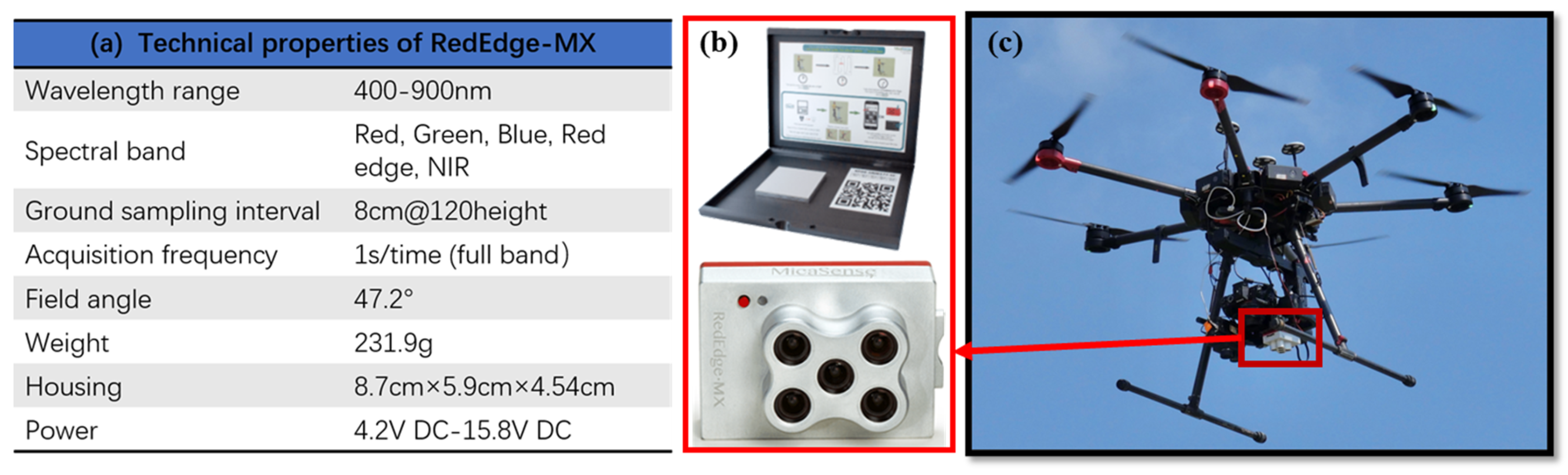
2.2. Data Acquisition

2.2.1. Canopy Spectral Data

A multispectral camera (RedEdge-MX, Micasense Co., Seattle, DC, USA) with center bands of 475, 560, 668, 717, and 840 nm mounted on a multi-rotor UAV (DJI-M600Pro, SZ DJI Technology Co., Ltd., Shenzhen, China) was used to acquire multispectral images of the experiment field (Figure 2). The flight mission was conducted between 10:00 and 14:00 under clear skies at five critical growth stages: V6 (9 July 2021), V8 (15 July 2021), V11 (26 July 2021), V16 (3 August 2021), and R1 (11 August 2021). There are 56 plots at V6, V8, V11, and R1, respectively, but only 48 plots at V16 due to an image missing; a total of 272 samples were collected. The flight height was 20 m above ground; the speed, navigation overlap, and side overlap were 1.7 m/s, 86%, and 75%, respectively. The resolution of the multispectral image is 0.01597 m, and the mission time is about 13 min. Radiation calibration was done by manually controlling the UAV at a certain height above the calibrated reflectance panel (clear and without shadows) for a few seconds before and after the UAV mission to acquire the corresponding panel image. The panel image was automatically calibrated using the Calibrate Reflectance tool on the Agisoft PhotoScan software (version 1.4.5, Agisoft LLC, St. Petersburg, Russia). Finally, the orthographic reflectance images were used to extract spectral features, texture features, and wavelet coefficient features.

2.2.2. Plant Measurements

The LCD was measured with Dualex Scientific+ (Force-A, Orsay, France) [41]. Yang et al. [42] showed that the average chlorophyll status of the ear-leaf, the first leaf above the ear, and the first leaf below the ear can be used to represent the canopy chlorophyll status in the reproductive stage. While at the vegetative stage, there was a good linear relationship between the canopy chlorophyll status and the average leaf chlorophyll status of the three spread leaves at the top of the plant [42]. In this study, the LCD of the ear-leaf, the first leaf above the ear, and the first leaf below the ear were measured with Dualex at the reproductive stage, while the LCD of the three spread leaves at the top of the plant was measured with Dualex at the vegetative stage. For each plot, eight rows were planted in a north-south direction, and the sampling locations were located at the center of each plot. LCD was acquired by measuring three plants; four positions at the middle part of each leaf were measured for each plant, and the average LCD was used as the LCD of the plot. LAI was collected using SunScan (Delta-T Devices Ltd., Cambridge, UK). Four directions (0°, 45°, 90°, and 135°) were measured for each plot, and each direction was measured three times. A total of 12 data points were measured for each plot, and the average value was used as the LAI value of the plot. Then the CCD was calculated based on the LCD and LAI with the method developed by Li et al. [43].

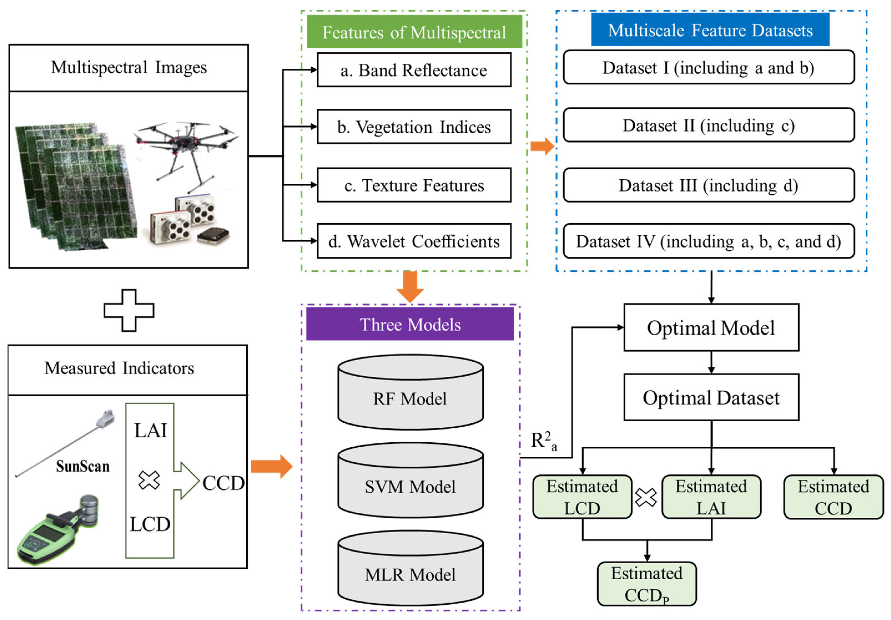
2.3. Data Processing

Figure 3 shows the methodology flowchart of this paper. It mainly contains three parts: the measured data, the model and method, and target parameters. The detailed steps are as follows:

(1)

Three types of image features were extracted from the multispectral features, and four multiscale datasets were constructed based on these three types of features;

(2)

Combining the estimation accuracy and efficiency of LCD, LAI, and CCD, the best estimation model was selected;

(3)

Based on the optimal model, the optimal fusion feature set for estimating CCD was evaluated;

(4)

After comparing the two CCD estimation results, the CCD mapping of the UAV scale was completed.

2.4. Multi-Scale Image Features

2.4.1. Vegetation Indices (VIs)

Thirteen chlorophyll-related vegetation indices and five-band reflectance (dataset I) were calculated from UAV multispectral images according to previous research (

Table 1. The VIs used in this study.

Vegetation Index	Formula	Reference
Normalize Difference Vegetation IndexKunakorn(NDVI)	$\left({\rho }_{NIR}-{\rho }_R\right)/\left({\rho }_{NIR}+{\rho }_R\right)$	[44]
Green Normalized Difference Vegetation Index (GNDVI)	$\left({\rho }_{NIR}-{\rho }_G\right)/\left({\rho }_{NIR}+{\rho }_G\right)$	[45]
Optimized Soil Adjusted Vegetation Index (OSAVI)	$\frac{\left(1+0.16\right)\left({\rho }_{NIR}-{\rho }_R\right)}{{\rho }_{NIR}+{\rho }_R+0.16}$	[13]
Red-edge Chlorophyll Index (CIrededge)	$\left({\rho }_{NIR}/{\rho }_{REG}\right)-1$	[16]
Structure-Insensitive Pigment IndexKunakorn(SIPI)	$\left({\rho }_{NIR}-{\rho }_B\right)/\left({\rho }_{NIR}-{\rho }_R\right)$	[46]
Enhanced Vegetation Index (EVI)	$\frac{2.5\times \left({\rho }_{NIR}-{\rho }_R\right)}{{\rho }_{NIR}+6\times {\rho }_R-7.5\times {\rho }_B+1}$	[47]
ROUPlant Pigment Ratio (PPR)	$\left({\rho }_G-{\rho }_B\right)/\left({\rho }_G+{\rho }_B\right)$	[48]
Red-edge NDVI (NDVIrededge)	$\left({\rho }_{NIR}-{\rho }_{REG}\right)/\left({\rho }_{NIR}+{\rho }_{REG}\right)$	[49]
MERIS Terrestrial Chlorophyll IndexKunakorn(MTCI)	$\left({\rho }_{NIR}-{\rho }_{REG}\right)/\left({\rho }_{REG}-{\rho }_R\right)$	[14]
Modified Chlorophyll Absorption Ratio Index (MCARI)	$\left({\rho }_{NIR}-{\rho }_R-0.2\times \left({\rho }_{REG}-{\rho }_G\right)\right)\times \left({\rho }_{REG}/{\rho }_R\right)$	[9]
Transformed Chlorophyll Absorption Reflectance Index (TCARI)	$3\times \left({\rho }_{REG}-{\rho }_R\right)-0.2\times \left({\rho }_{REG}-{\rho }_G\right)\times \frac{{\rho }_{REG}}{{\rho }_R}$	[50]
Combined Index (TCARI/OSAVI)	$TCARI/OSAVI$	[51]
Difference Vegetation Index (DVI)	$\left({\rho }_{NIR}-{\rho }_R\right)$	[52]

Note: ${\rho }_R$ represents the reflectance of the red band, ${\rho }_G$ represents the reflectance of the green band, ${\rho }_B$ represents the reflectance of the blue band, ${\rho }_{NIR}$ represents the reflectance of the near infrared band, and ${\rho }_{REG}$ represents the reflectance of the red-edge band.

). These VIs were regarded as components of multi-scale features and as input features of the CCD estimation model. The VIs of each plot were obtained by averaging the vegetation indices of all pixels in each plot. The correlation coefficients (r) between the VIs and the LCD, LAI, and CCD were calculated. Then, the VIs were sorted according to the correlation coefficients.

2.4.2. Texture Features

Eight texture features were extracted using a gray level co-occurrence matrix [53], including average value, variance, uniformity, contrast, difference, entropy, second moment, and correlation (

Table 2. Texture features extracted from multispectral images.

GLCM-Based Feature	Abbreviation	Formula
Mean Value	MEAN	$\mathrm{M}\mathrm{E}\mathrm{A}\mathrm{N}={\sum }_{i,j}^{N-1}i\times p\left(i,j\right)$
Variance	Var	$\mathrm{V}\mathrm{a}\mathrm{r}={\sum }_{i=0}^{N-1}{\sum }_{j=0}^{N-1}p\left(i,j\right){\left(i-\mu \right)}^2$
Homogeneity	Hom	$\mathrm{H}\mathrm{o}\mathrm{m}={\sum }_{i=0}^{N-1}{\sum }_{j=0}^{N-1}\frac{p\left(i,j\right)}{1+{\left(i-j\right)}^2}$
Contrast	Con	$\mathrm{C}\mathrm{o}\mathrm{n}={\sum }_{i=0}^{N-1}{\sum }_{j=0}^{N-1}p\left(i,j\right){\left(i-j\right)}^2$
Dissimilarity	Dis	$\mathrm{D}\mathrm{i}\mathrm{s}={\sum }_{i=0}^{N-1}{\sum }_{j=0}^{N-1}p\left(i,j\right)|i-j|$
Entropy	Ent	$\mathrm{E}\mathrm{n}\mathrm{t}=-{\sum }_{i=0}^{N-1}{\sum }_{j=0}^{N-1}p\left(i.j\right)\log \left(p\left(i,j\right)\right)$
Angular Second Moment	ASM	$\mathrm{A}\mathrm{S}\mathrm{M}={\sum }_{i=0}^{N-1}{\sum }_{j=0}^{N-1}{\left\{p\left(i,j\right)\right\}}^2$
Correlation	Cor	$\mathrm{C}\mathrm{o}\mathrm{r}={\sum }_{i=0}^{N-1}{\sum }_{j=0}^{N-1}\frac{\left(i-{\mu }_i\right)\left(j-{\mu }_j\right)}{{\sigma }_i{\sigma }_j}$

Note: where $N$ is the number of gray levels; $p$ is the normalized symmetric gray level co-occurrence matrix of dimension $N\times N$; $p\left(i,j\right)$ is the $\left(i,j\right)$ element of $p$; ${\mu }_i={\sum }_{i=0}^{N-1}{\sum }_{j=0}^{N-1}i\times p\left(i,j\right)$; and ${\sigma }_i=\sqrt{{\sum }_{i=0}^{N-1}{\sum }_{j=0}^{N-1}p\left(i,j\right){\left(i-{\mu }_i\right)}^2}$.

). The texture features of each plot were extracted from five single bands with a 7 × 7 window size. A total of 40 texture features were calculated for each growth stage (dataset II), and the texture feature most highly correlated with LCD, LAI, and CCD will be selected as a component of multi-scale features.

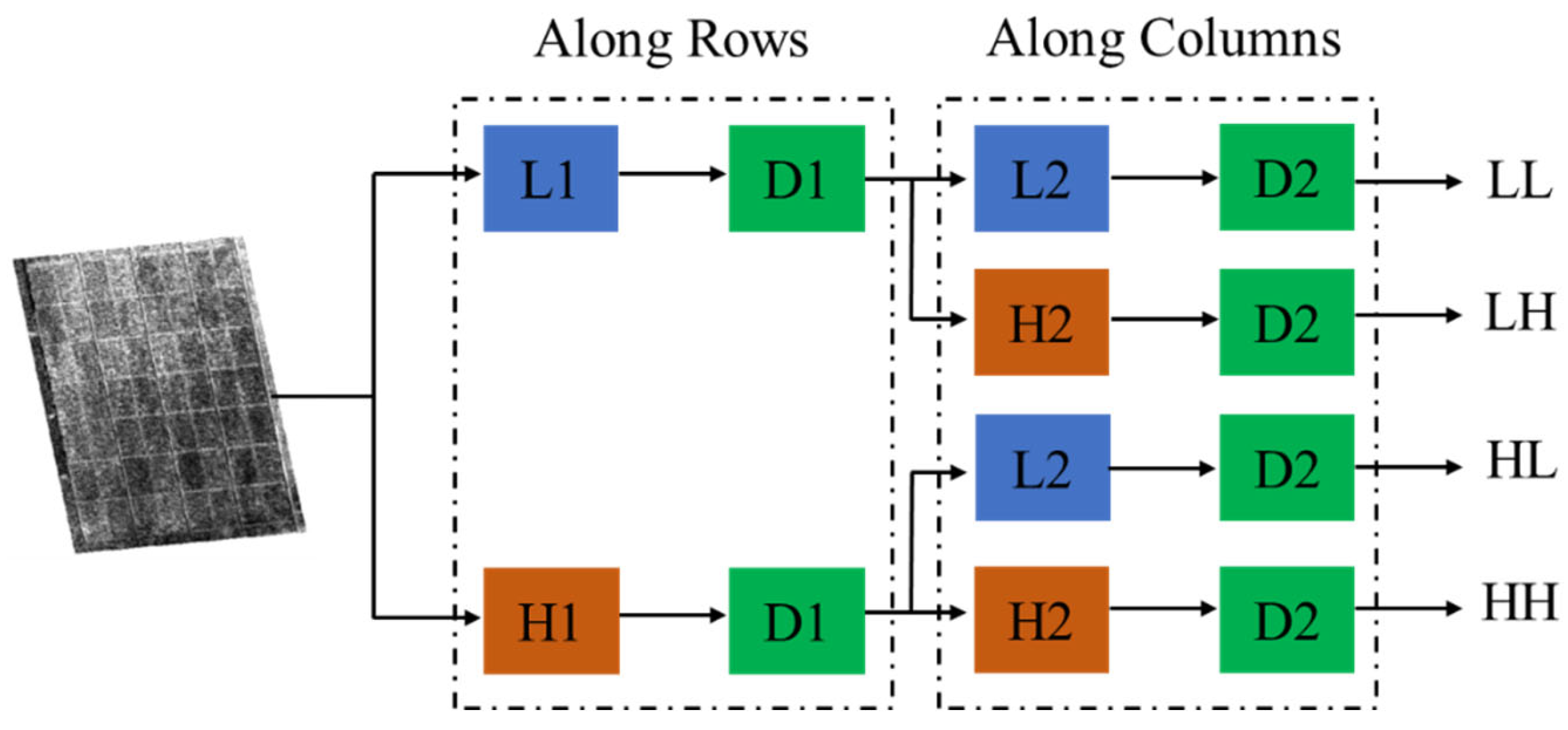
2.4.3. Discrete Wavelet Transformation (DWT)

The DWT is a signal decomposition method that transforms the original signal into the frequency domain with a base function (mother wavelet function) and has been widely used to extract signal features [26,54,55]. The bior1.3 wavelet basis function was selected in the study. The decomposition process is shown in Figure 4. Based on the one-dimensional low-pass filter (L1), the input image was subjected to row convolution and downsampling (D1), and the obtained image was subjected to column convolution and downsampling (D2) with the one-dimensional low-pass filter (L2), and then the approximate sub-image (LL) can be obtained. Similarly, we can also obtain the horizontal detail sub-image (LH), the vertical detail sub-image (HL), and the diagonal detail sub-image (HH). The reflectivity image of each band of the UAV multispectral image was transformed into a wavelet involving four sub-images [19]. A total of 20 discrete wavelet coefficients were calculated for each growth stage (dataset III).

2.4.4. Construction of a Multi-Scale Image Feature Dataset

The band reflectance and VIs were unified as the spectral feature category of the image. Texture features represent the spatial information of the image, and wavelet features represent the frequency and spectral details of the image [56,57]. In this study, the dataset Ⅰ, the dataset Ⅱ, and the dataset Ⅲ were integrated to construct the dataset Ⅳ (

Table 3. Description of the four feature datasets.

Feature Dataset	Band + VI	Texture	Wavelet
Ⅰ	√	×	×
Ⅱ	×	√	×
Ⅲ	×	×	√
Ⅳ	√	√	√

). The training set and validation set of each dataset were divided by a proportion of 7:3. The training set is composed of 196 samples, and the validation set is composed of 76 samples.

2.5. Estimation Methods

Three types of methods were selected to build the estimation models of LCD, LAI, and CCD, including multivariable linear regression (MLR), support vector regression (SVM), and random forest regression (RF).

MLR is a statistical technique that estimates dependent variables (such as LCD, CCD, and LAI) using the combination of multiple independent variables (such as Vis and texture features) [38,58,59]. It is an effective, simple, and practical method to estimate the target variables by the optimal combination of multiple independent variables [60].

SVM is a commonly used nonlinear kernel function [38,61,62]. The SVM method outperformed other machine learning methods when the dataset was small. This study selected the RBF kernel function, which has two very important parameters: penalty parameter C and kernel parameter g. The penalty parameter C represents the tolerance of the model to errors in order to achieve a balance between model accuracy and model complexity [61]. The kernel parameter g controls the regression error of the model and affects the complexity of the distribution of the sample data in the high-dimensional feature space [62]. The above parameters were determined by MATLAB R2017a (version 9.2, Math Works, Inc., Natick, MA, USA) software [39,63].

Random forest (RF) regression is a nonparametric regression technique based on the decision tree method and bagging method [38,64]. Additionally, RF has the capacity to efficiently process massive data and complex nonlinear relationships and is safe from information redundancy and overfitting [38,61,65]. The RF model establishes multiple unrelated decision trees by randomly sampling samples and features and obtains the prediction results in a parallel manner. Each decision tree can obtain an estimation result through the samples and features extracted, and the regression estimation result of the whole forest can be obtained by averaging the results of all trees. The TreeBagger function provided by MATLAB R2017a software was used in the random forest method. Its main parameters are the minimum leaf size (minleaf) and the number of decision trees (ntree). In this study, the minleaf and ntree parameters were set at 5 and 800, respectively. Therefore, they were used in this study to evaluate the potential of multi-scale feature fusion in maize chlorophyll content estimation.

2.6. Precision Evaluation

The coefficient of determination (R²), root mean square error (RMSE), and normalized RMSE (NRMSE) were used to evaluate the performance of the models. In addition, the adjusted coefficient of determination (R²_a) was introduced to decrease the influence of the sample size (n) and the number of independent variables (k). The value of the R²_a will not get closer to 1 due to the increase in the number of independent variables in the regression [66,67]. The formulas of R², RMSE, NRMSE, and R²_a are shown as Equations (1–4):

$${\mathrm{R}}^2=\frac{\sum _{\mathrm{i}}^{\mathrm{n}}(\widehat{{\mathrm{y}}_{\mathrm{i}}}-\stackrel{\_}{\mathrm{y}})}{\sum _{\mathrm{i}}^{\mathrm{n}}({\mathrm{y}}_{\mathrm{i}}-\stackrel{\_}{\mathrm{y}})}$$

(1)

$$\mathrm{R}\mathrm{M}\mathrm{S}\mathrm{E}=\sqrt{\frac{\sum _{\mathrm{i}=1}^{\mathrm{n}}{\left(\widehat{{\mathrm{y}}_{\mathrm{i}}}-{\mathrm{y}}_{\mathrm{i}}\right)}^2}{\mathrm{n}}}$$

(2)

$$\mathrm{N}\mathrm{R}\mathrm{M}\mathrm{S}\mathrm{E}=\frac{\mathrm{R}\mathrm{M}\mathrm{S}\mathrm{E}}{{\mathrm{y}}_{\mathrm{m}\mathrm{a}\mathrm{x}}-{\mathrm{y}}_{\mathrm{m}\mathrm{i}\mathrm{n}}}$$

(3)

$${\mathrm{R}}_{\mathrm{a}}^2=1-\left[\left(1-{\mathrm{R}}^2\right)\left(\frac{\mathrm{n}-1}{\mathrm{n}-\mathrm{k}-1}\right)\right]$$

(4)

where $\widehat{{\mathrm{y}}_{\mathrm{i}}}$ is the predicted CCD, ${\mathrm{y}}_{\mathrm{i}}$ is the measured CCD, $\stackrel{-}{\mathrm{y}}$ is the average measured CCD, ${\mathrm{y}}_{\mathrm{m}\mathrm{a}\mathrm{x}}$ is the maximum value of the CCD, ${\mathrm{y}}_{\mathrm{m}\mathrm{i}\mathrm{n}}$ is the minimum value of the CCD, n is the number of samples, and k is the number of independent variables.

3. Results and Analysis

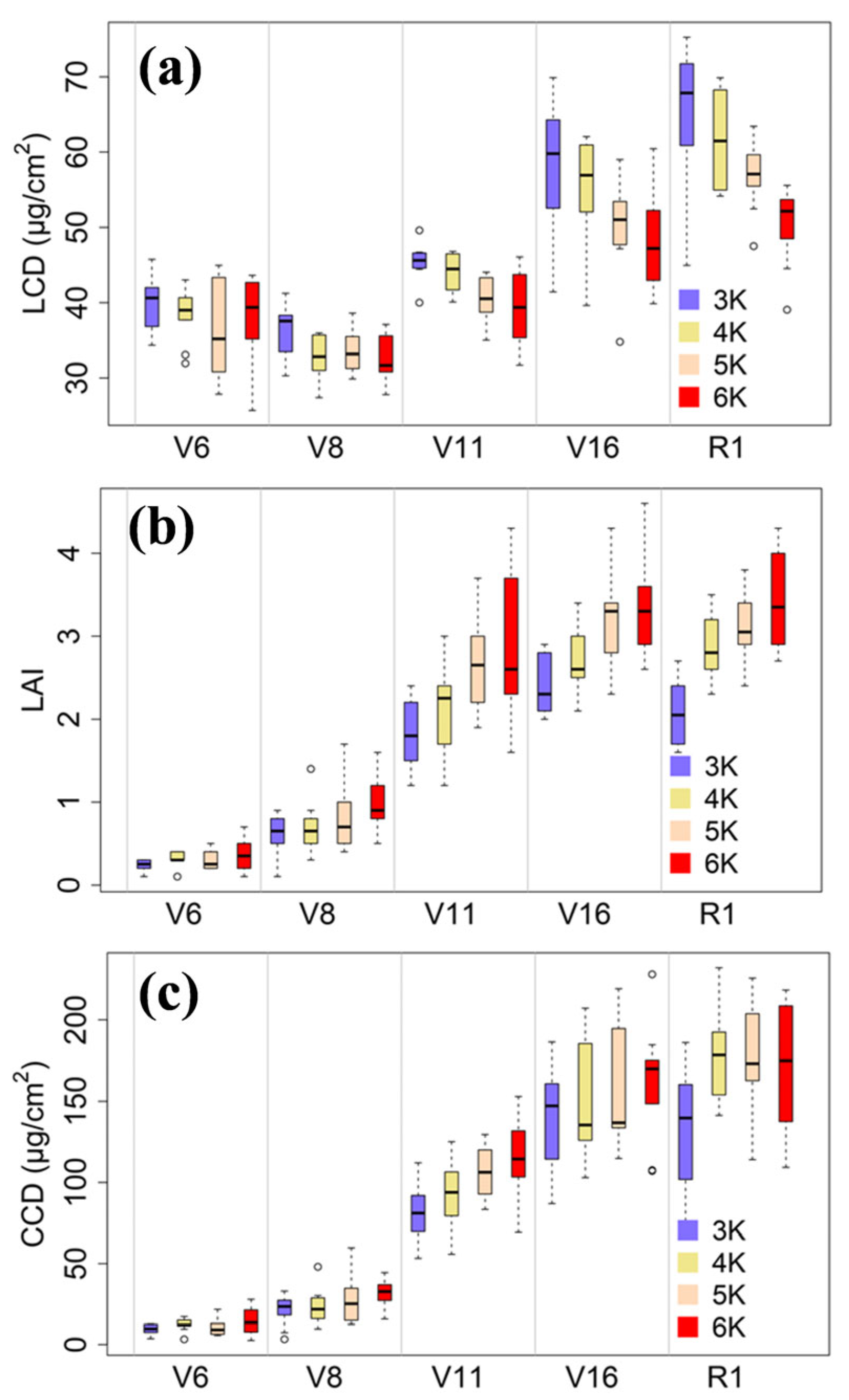
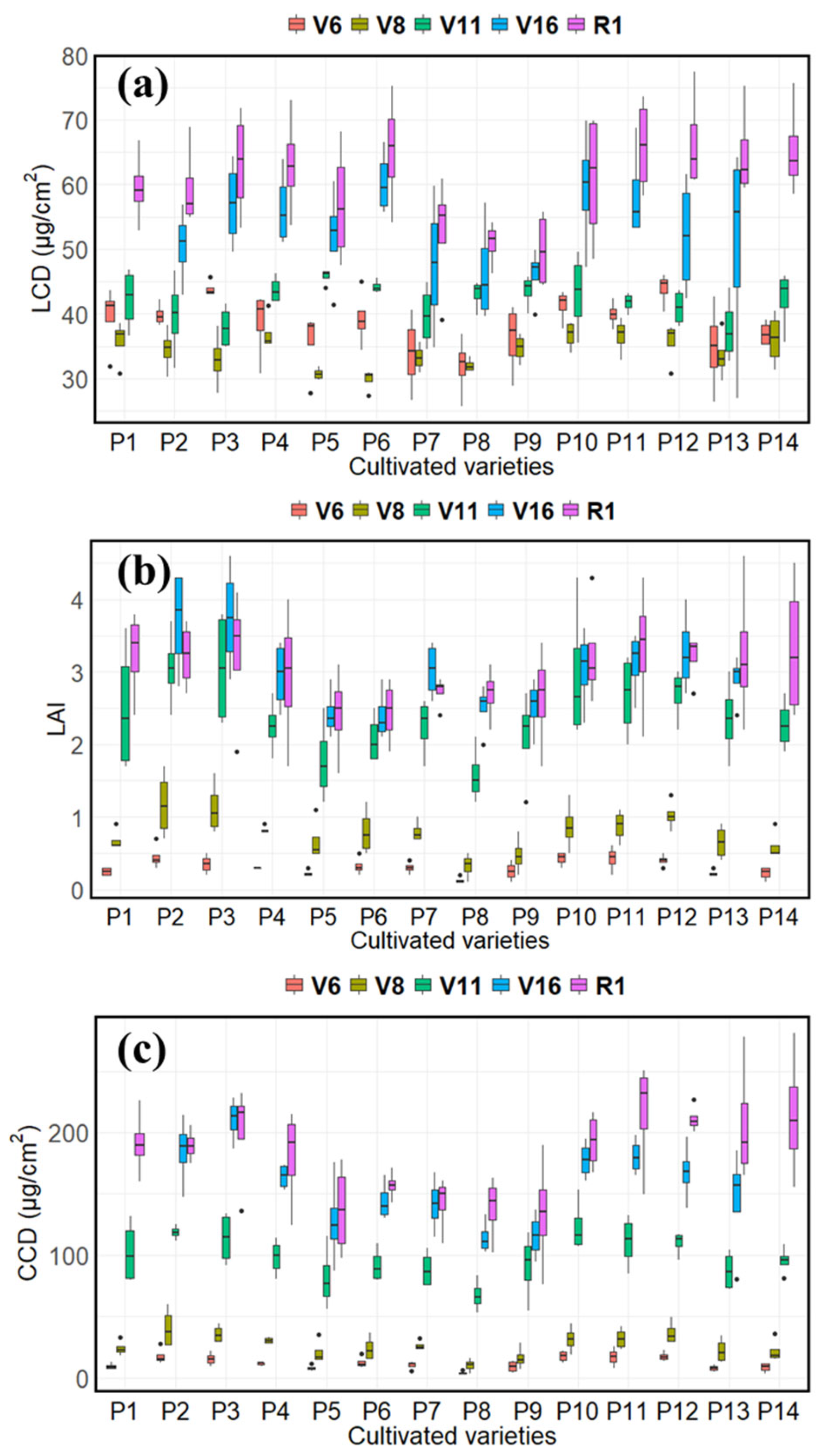
3.1. Dynamic Changes of the LCD, LAI, and CCD

The dynamic changes of LCD, LAI, and CCD at the whole growth stage and under different planting densities are shown in Figure 5. The results showed that the LCD, LAI, and CCD increased with the growth of maize. At the same growth stage, LCD was inversely proportional to density (Figure 5a), but LAI was proportional to density (Figure 5b). This phenomenon was not obvious at the early stages (V6 and V8) of maize growth but became significant at the later stages (V11, V16, and R1). Although CCD was the product of LAI and LCD, it was more affected by LAI and was proportional to the density at the same growth stage (Figure 5c). Figure 6 shows the changes in LCD, LAI, and CCD under different varieties and different growth stages. The results show that the LCD, LAI, and CCD of different varieties gradually increased with the growth of maize plants, but there were differences among varieties. As shown in Figure 6a, the differences of the LCD, LAI, and CCD among different varieties were small, but the differences of the LCD, LAI, and CCD among different varieties were larger after V11.

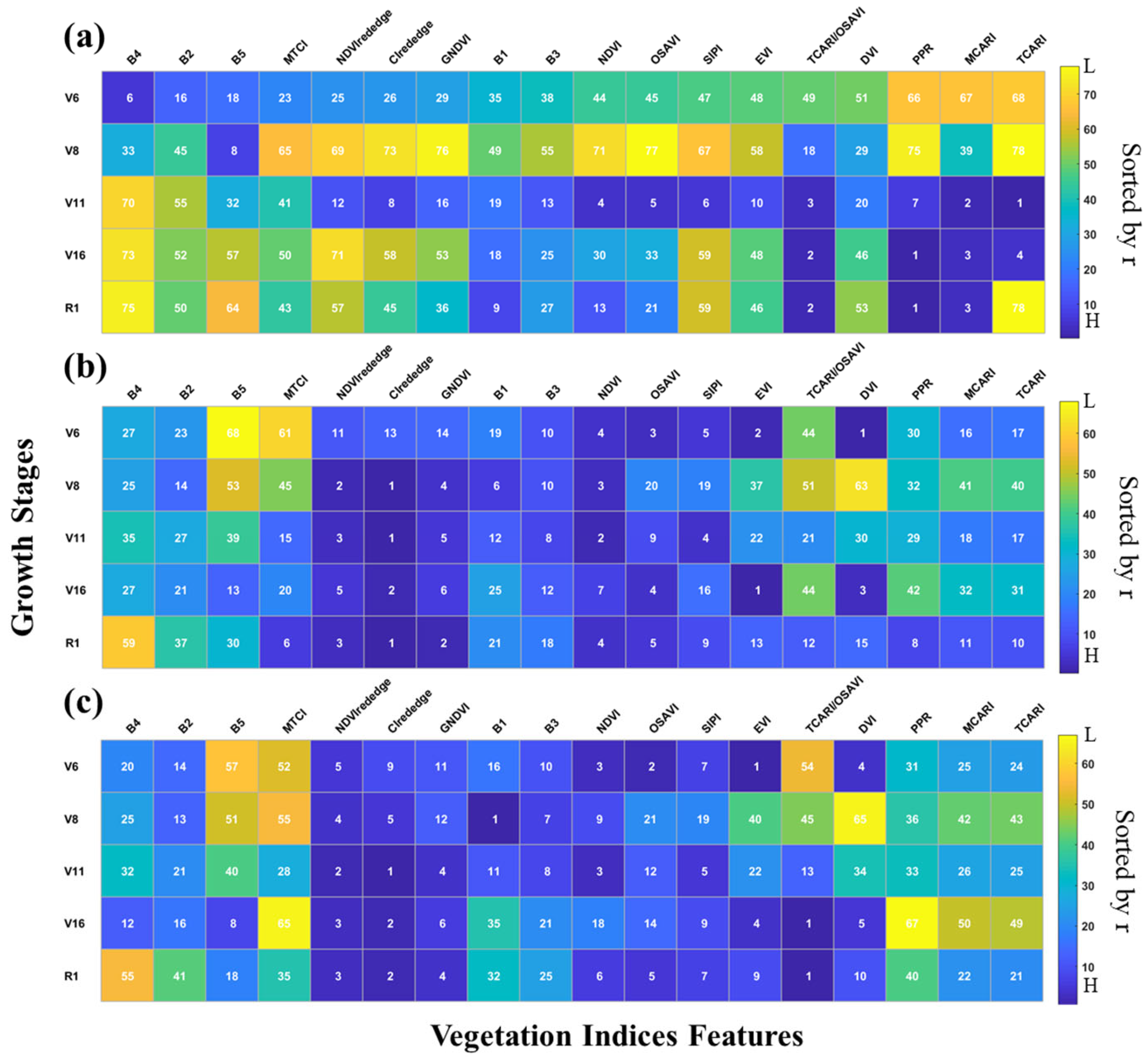
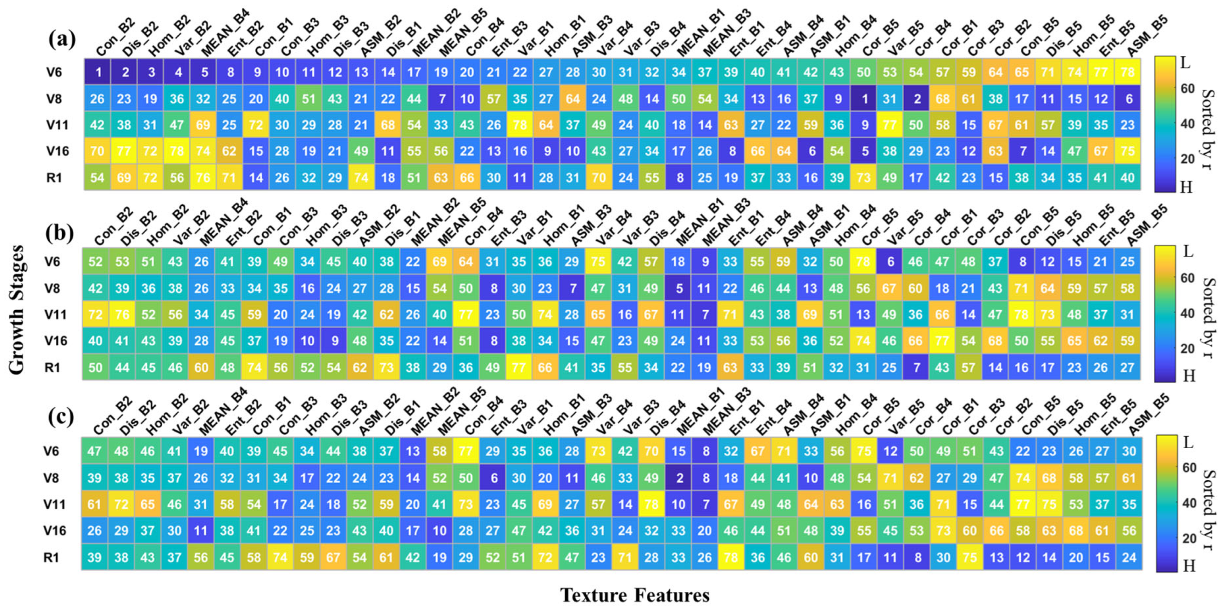
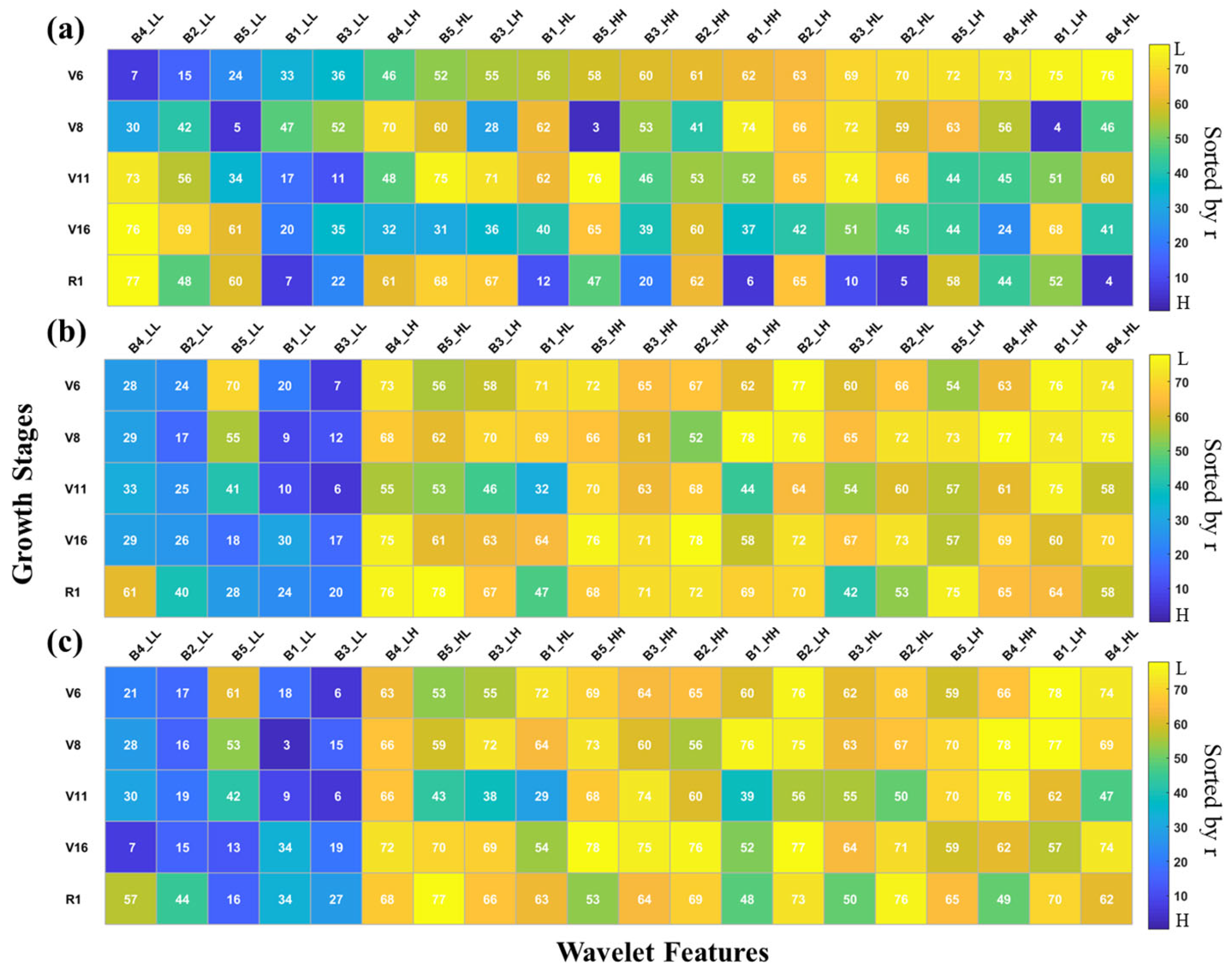
3.2. Correlation Analysis of Image Features at Different Growth Stages

The correlation (correlation coefficient, r) between target variables (LCD, LAI, and CCD) and three types of features (vegetation indices, wavelets, and textures) was analyzed and sorted, and the results are shown in Figure 7, Figure 8 and Figure 9. For each growth stage, a total of 78 features were sorted according to the r values from high to low. The results showed that the correlation between target variables and different feature types is quite different at different growth stages. The correlation between LCD and vegetation indices, texture, and wavelet coefficient had great differences at the whole growth stage and presented a certain regularity with the growth stage (the maximum r between LCD and vegetation indices is 0.28–0.69, the maximum r between LCD and texture is 0.36–0.53, and the maximum r between LCD and wavelet is 0.22–0.50). As shown in Figure 7a, the correlation between band reflectance (such as B4, B2, and B5) and LCD is high at the early growth stage (V6 and V8) but poor at the late stage (V11, V16, and R1). The VIs with high correlation at the early growth stage (V6 and V8) did not perform well at the late growth stage (V11, V16, and R1), such as PPR, MCARI, and TCARI. As shown in Figure 8a, for the texture features (Con_B2, Dis_B2, Hom_B2, Var_B2, and Mean_B4) with better correlation with LCD at the V6 stage, the correlation between these texture features and LCD decreased with the growth process. They were not obviously different at the whole growth stage for the correlation between LAI and vegetation indices, texture, and wavelet coefficient (the maximum r between LAI and vegetation indices is 0.77–0.91, the maximum r between LAI and texture is 0.64–0.84, and the maximum r between LAI and wavelet is 0.47–0.84). As shown in Figure 9a, some wavelet features (such as B4_LL and B5_LL) yielded better correlation with LCD at the early stage (V6 and V8) than at the later growth stage (V11, V16, and R1). While some wavelet features (such as B1_HH and B2_HL) were poorly correlated with LCD at the early stage (V6, V8, and V11), they yielded a higher correlation with LCD at the later stage (V16 and R1). The vegetation indices yielded a higher correlation with LAI than that of the texture features and wavelet coefficients (Figure 7b). There were some texture features and wavelet coefficients that were highly correlated with LAI at each growth stage (Figure 8b and Figure 9b), which indicated the importance of texture features and wavelet features to LAI. The correlation between CCD and vegetation indices (Figure 7c), texture features (Figure 8c), and wavelet coefficients (Figure 9c) were basically consistent with that of LAI (the maximum r between CCD and vegetation indices is 0.70–0.87, the maximum r between CCD and texture is 0.51–0.85, and the maximum r between CCD and wavelet is 0.34–0.84). The value of the correlation coefficient is shown in the Supplementary Materials (Tables S1–S3).

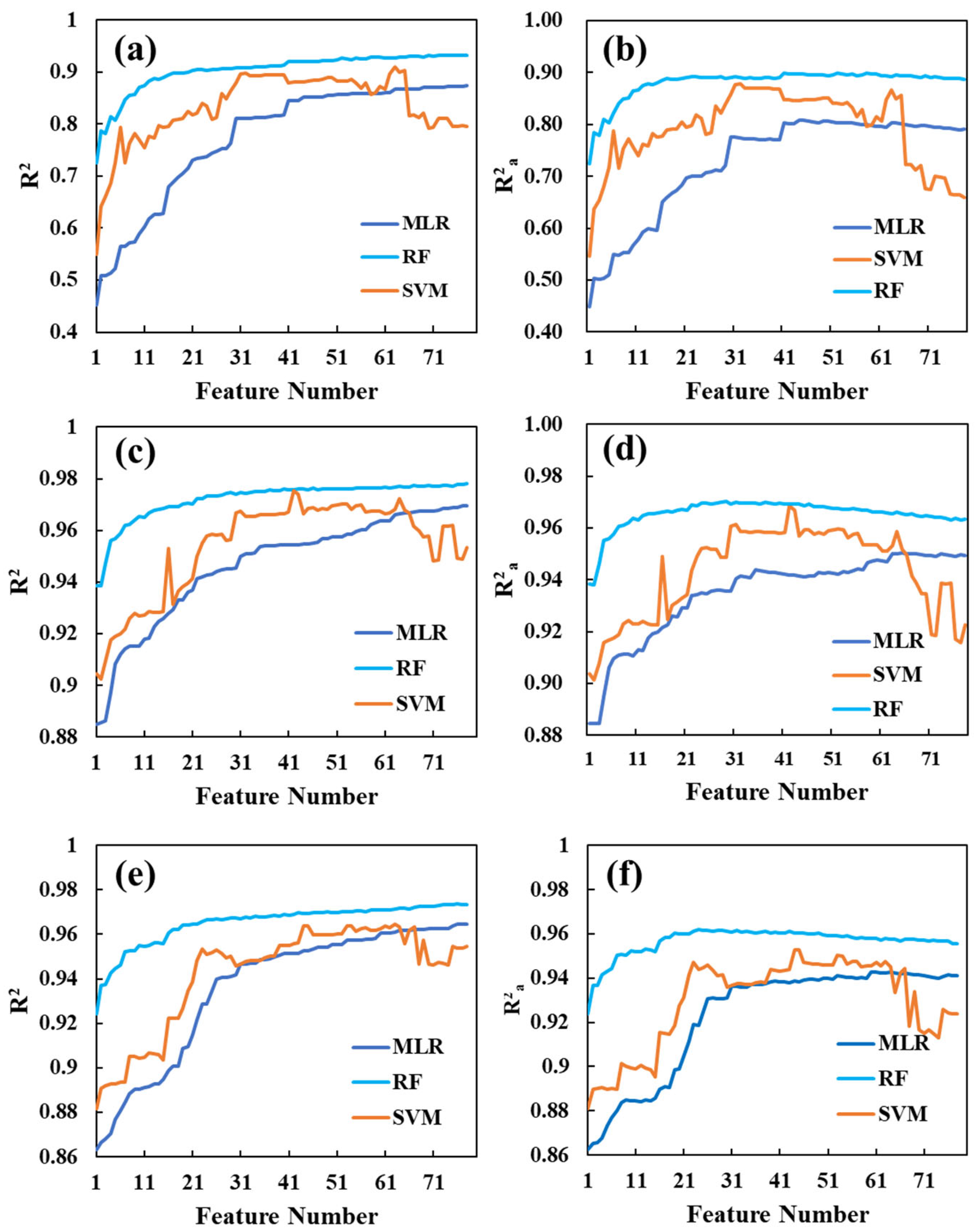
3.3. Estimation Results of LCD, LAI, and CCD

In order to explore the optimal machine learning method for CCD mapping at the whole growth stage, three machine learning methods were selected to develop a CCD estimation model by integrating spatial features (texture and wavelet features) and spectral features. R² and R²_a of the three machine learning methods are shown in Figure 10. Compared with the SVM and MLR methods, the RF method had the highest stability and accuracy. For the RF method, R² always increased with the increase in the number of feature parameters, while R²_a first increased and then stabilized with the increase in the number of feature parameters. Thus, the adjusted determination coefficient (R²_a) was used to evaluate the performance of each CCD estimation model and determine the number of input features. In the estimation of CCD, the R²_a of the RF model can reach 0.96, and the model performance was the most stable compared with SVM and MLR, which can reach the best performances under the premise of minimum feature quantity. For the estimation of LCD and LAI, the RF model also yielded the best performance, with R²_a equal to 0.89 and 0.97, respectively. Therefore, the RF method was finally selected to estimate LCD, LAI, and CCD. The RF method was used to estimate LCD, LAI, and CCD from four different datasets. According to R²_a and correlation ranking, it was determined that the best input characteristics of the model for Ⅰ, Ⅱ, Ⅲ, and Ⅳ datasets were the top 16, 18, 16, and 24, respectively.

LCD, LAI, and CCD were estimated from four datasets using the RF method. The estimation results of LCD, LAI, and CCD are shown in

Table 4. Four feature sets were used for RF method estimation of LCD, LAI, and CCD.

Index	Feature Set	R2	RMSE (μg/cm2)	NRMSE (%)
LCD	Ⅰ	0.90	6.70	14.32
	Ⅱ	0.90	7.20	15.88
	Ⅲ	0.86	10.04	22.15
	Ⅳ	0.91	6.59	14.51
LAI	Ⅰ	0.97	0.37	20.18
	Ⅱ	0.96	0.43	23.28
	Ⅲ	0.96	0.42	22.62
	Ⅳ	0.97	0.35	18.76
CCD	Ⅰ	0.96	26.22	28.26
	Ⅱ	0.95	33.24	35.84
	Ⅲ	0.95	40.42	43.58
	Ⅳ	0.97	24.85	26.78

Note: R² represents the determination coefficient of the training set, and (N)RMSE represents the (relative) root mean square error of the validation set.

. The RF method trained over different datasets yielded a high and similar performance for LCD, with R² ranged between [0.86, 0.91] and RMSE ranged between [6.59, 10.04]. The LCD estimation model trained over dataset IV achieved the optimal estimation with the highest R² (0.91) and the lowest RMSE (6.59 μg/cm²). It proved the advantages of multi-scale image feature fusion. Similarly, the RF method trained over different datasets yielded a high and similar performance for LAI estimation, with an R² ranging between [0.96, 0.97] and an RMSE ranging between [0.35, 0.43]. The LAI estimation model trained over dataset IV also achieved the best estimation, with the highest R² (0.97) and the lowest RMSE (0.35).

For the estimation of CCD, the RF model trained over four feature datasets yielded good performance, with R² ≥ 0.95 (Table 4). The model trained over dataset Ⅳ yielded the best performance, with R² = 0.97 and RMSE = 24.85 μg/cm². The results indicated that the optimal input feature set of the LCD, LAI, and CCD estimation models was IV, and multi-scale image feature fusion improved the estimation accuracy. In addition, the errors of CCD under different varieties were analyzed based on the RF and IV datasets, as shown in Figure 11. The difference in varieties had little effect on the CCD estimation, and the overall difference was small. The difference in P11, P12, and P13 was slightly larger than the other varieties, mainly due to the significant underestimation caused by the high-density plots of these three varieties in the late growth stage, leading to a large overall error.

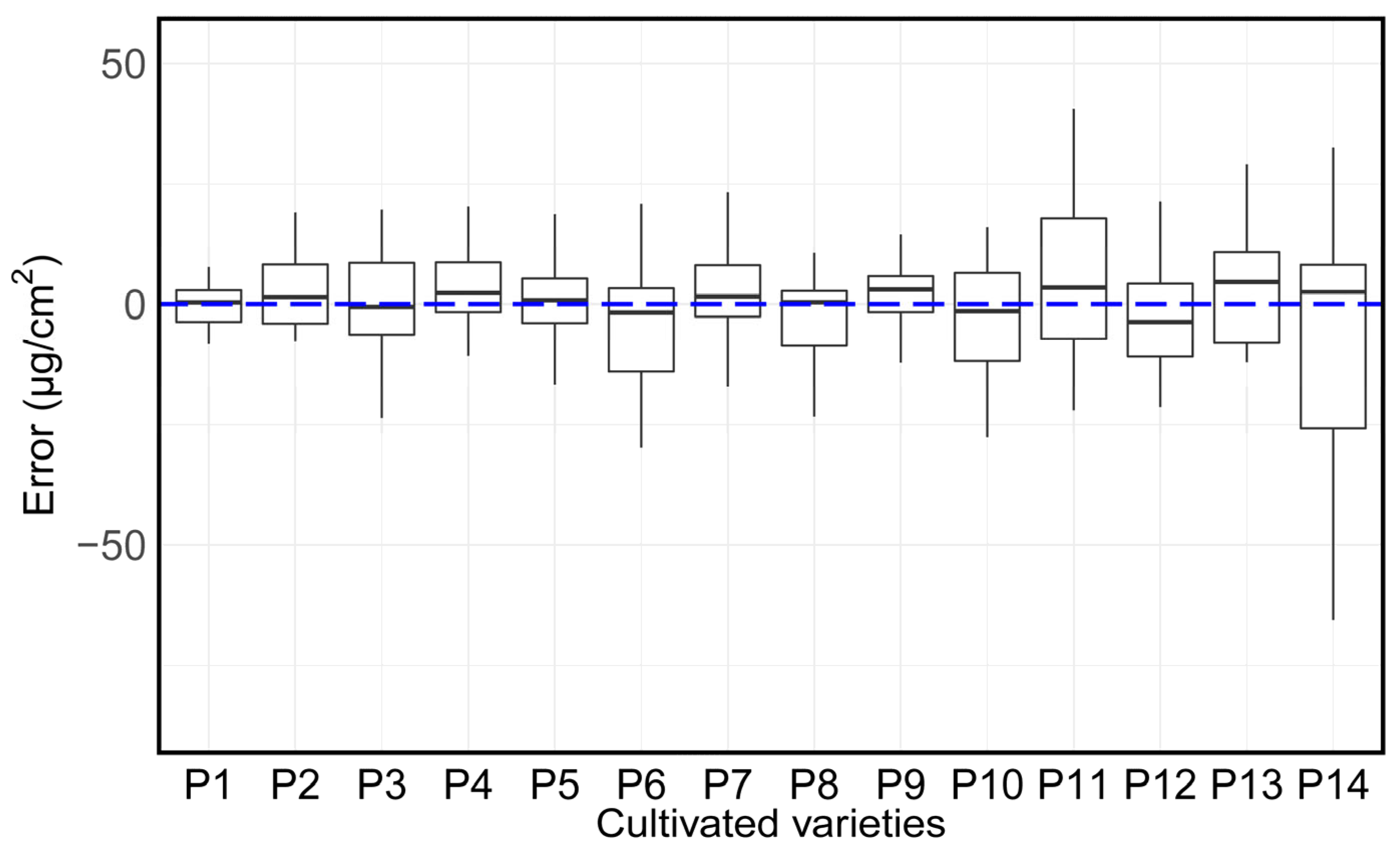
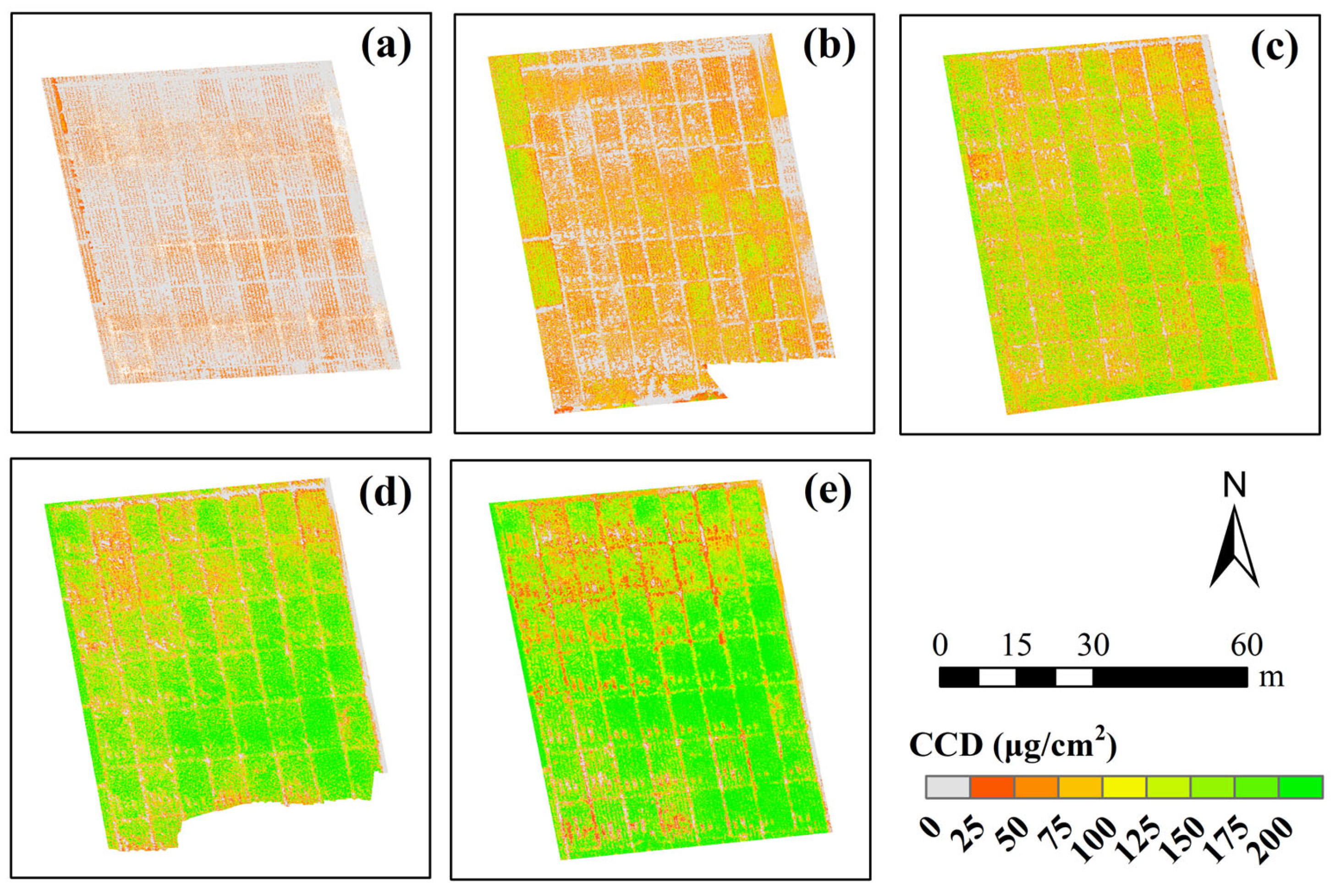
3.4. CCD Calculated Based on the Estimation Results of LCD and LAI

The LCD and LAI were estimated separately using the RF model and dataset Ⅳ, and the CCD calculated by multiplying the estimated LCD and LAI was expressed as CCD_P. The direct estimation results of CCD and the indirect estimation results of CCD_P were shown in Figure 12. The two CCD estimation methods both yielded good performances. The R² and RMSE of the direct estimation model of CCD were 0.96 and 24.85 μg/cm², while those of the estimation model of CCD_P were 0.97 and 26.85 μg/cm². The accuracy of CCD estimation combined with the RF model on dataset IV was slightly better than that of CCD_P. In addition, both methods had good estimation performance when the chlorophyll content was low. When the chlorophyll content was high, the two methods were slightly underestimated. The reason may be that the data range of the validation set is beyond the range of the training set, and the model has not learned relevant information.

The map of the spatial distribution of CCD under different varieties and densities was created using UAV multispectral images (Figure 13). The CCD value at the V6 stage was low, not more than 75 μg/cm². Since the V8 stage, the value of CCD has increased significantly. The CCD value of high-density processing was much higher than that of low-density processing. CCD mapping using the optimal model and the multi-scale image feature dataset of the UAV can directly reflect the spatial distribution of CCD at different growth stages and densities.

4. Discussion

Generally, when estimating the CCD of maize, it is easy to be affected by canopy structure (such as LAI) or planting density, resulting in the LCD information being ignored [68]. Figure 5 implied that LCD decreased with the increase of density at the same growth stage as LAI and CCD increased with the increase of density, and CCD showed the same trend as LAI. With the increase in density, the population of plants grows vigorously (reflected in high LAI and high CCD) [69]. However, under the condition of high density, due to poor ventilation and light transmission, the field is shaded, and the photosynthesis becomes poor, resulting in poor growth of single maize (reflected in low LCD).

Figure 7, Figure 8 and Figure 9 implied that the correlation between texture features and LCD was the highest at the early growth stage (V6), which was superior to vegetation indices and wavelet coefficients. The main reason may be that the small size of early maize plants and more exposed soil interfere with the response of the canopy spectrum to the chlorophyll characteristics of individual maize. Spectral heterogeneity was a main reason for the low correlation between vegetation indices and LCD in the V6 stage. The texture features were sensitive to the boundary between soil and green plants [70], and the corresponding texture features and LCD displayed a high correlation at the early stage (V6). The vegetation indices had the best correlation with LAI at the whole growth stage because the canopy spectrum was always proportional to the maize population and was less affected by the soil. At each growth stage, there are wavelet features highly related to the target variables. DWT can effectively separate useful information from weak information, thus leading to efficient utilization of available information [27]. This is one of the reasons why wavelet features were introduced.

In this study, four different feature datasets and three machine learning methods were used to estimate LAI, LCD, and CCD. The optimal LAI, LCD, and CCD estimation was obtained by integrating the RF model and dataset Ⅳ. The main reason may be that the dataset Ⅳ combines the spectral, frequency, and spatial information of the multispectral image, making up for the defect of using only spectral or spatial features. Many studies have shown that multi-feature fusion, which includes wavelet features, texture features, and vegetation indices, can improve the estimated accuracy of target variables [22,27]. Therefore, on the one hand, Figure 14 presents the change of three indicators (Cor_B5, MTCI, and B3_LL) with growth stage and density. The correlation between MTCI and LCD was the best among all test indicators, which was consistent with previous studies [71,72]. MTCI was in direct proportion to the growth stage and density, especially at the late growth stage (Figure 14a). Obviously, in the same growth stage, the relationship between MTCI and density is opposite to that between LCD and density. Therefore, although many studies use UAV multispectral features to monitor CCD [73], using vegetation index features alone to estimate CCD may miss the change in LCD. As shown in Figure 14b, the B3_LL was the wavelet coefficient with the best correlation with LAI and CCD. It decreased gradually with the increase in density at the same growth stage, which was more obvious at the early stages (V6 and V8). The relationship between B3_LL and growth stage was consistent with the relationship between B3_LL and density, which was the same as LAI and CCD (both positive or negative). As shown in Figure 14c, Cor_B5 was the texture feature that had the best correlation with the LCD. Additionally, Cor_B5 was in direct proportion to the growth stage, except that it was not obvious in the V8 and V11 stages. At the same growth stage, Cor_B5 decreased with the increase in density, except for different R1 stages. The change of Cor_B5 with growth stage and density was similar to that of LCD. Previous researchers have rarely used texture features for chlorophyll research, but this paper’s analysis shows that, compared with vegetation indices and wavelet features, texture features may have more advantages in the representation of LCD information. It proved that the dataset IV can realize the optimal estimate, and multi-scale feature fusion is an important way to improve the accuracy of CCD estimation [19,32,74,75]. On the other hand, taking the dataset Ⅳ as the input to the estimation of the CCD model, VIs features account for 54% of the effective input features, texture features account for 29% of the effective input features, and wavelet features account for 17% of the effective input features. The combination of these features improved the contribution rate for a certain type of feature so as to improve the accuracy of model estimation. The proportion of different feature types in effective features also proved the necessity of fusing multiple image features. Compared with SVM and MLR models, the RF model is good at dealing with high-dimensional data and complex nonlinear problems and has randomicity and strong generalization ability [76]. Although SVM can deal with nonlinear problems, it is more sensitive to the number of input features and takes more time as compared with the RF model (Figure 10). MLR is a multiple linear regression model, which relies on the linear relationship between multiple independent variables and dependent variables for modeling [77]. Thus, the MLR makes it difficult to solve complex nonlinear problems. Figure 10 presents the unique advantages of the RF model under different feature numbers, with strong stability and high accuracy. The time taken for the RF model to reach the optimal estimate on different datasets differs by less than one second, and the time taken on the dataset IV with the largest number of input features was 2.04 s (Figure S1 in the Supplementary Materials). The RF model can still maintain high operational efficiency with a large number of inputs. The RF method is the optimal consideration when the trade-offs of model complexity, stability, accuracy, and efficiency issues are combined [78,79]. The number of input features in the model was determined according to the best R²_a. In this study, when the number of input features increases to a certain value, the increase in the number of features will not improve the accuracy but will lead to a decrease in accuracy. Therefore, determining the optimal number of input features for the model reduces information redundancy, thus improving the operational efficiency and estimation accuracy of the model.

In this study, two strategies were used to estimate CCD. The results demonstrated that the estimation results of CCD_P and CCD were similar, but the direct CCD estimation model yielded slightly higher performance than that of CCD_P. The main reason may be that there is a double error transmission in estimating CCD_P using the estimation results of LCD and LAI [80], resulting in a slightly lower estimation accuracy of CCD_P as compared with the CCD estimation model. It was noted that both models showed a general underestimation at higher CCD values, mainly due to the fact that these plots were high density plots (6K) at the R1 stage, when the leaves are no longer growing substantially and the canopy structure also reaches its peak, and the relatively dense upper leaves block the lower ones, resulting in the inability to highlight the spectral characteristics of the whole canopy and the reflectance shows saturation, which eventually affected the CCD estimation [81]. In the future, the estimation accuracy of CCD_P may be improved by seeking more effective feature extraction and fusion methods. This research is based on the analysis of the data for the whole growth stage of maize and integrates multi-scale features and machine learning methods to estimate LCD, LAI, and CCD. Although better estimation accuracy can be obtained, it only performs simple fusion for limited image features. Multi-level fusion of multi-scale image features can be considered to improve the contribution of the LCD in CCD estimation. The CCD estimation method proposed in this study was applicable to the estimation of LCD, LAI, and CCD under different densities, different varieties, different growth stages, and clear weather conditions. The effects of different regions and differences in weather conditions were not considered, and the scalability of the model in different regions and its adaptability to different weather conditions can be explored by considering a larger area of plots as the basis of the study in the future. In addition, the CCD estimation model built based on the data of the whole growth stage may vary in specific time scenario applications. In the future, the data collected at different regions and different years will be used to develop a universal model suitable for different growth stages to improve the time scalability of the model.

5. Conclusions

In this study, the LCD, LAI, and CCD models were developed using three machine learning methods with four different feature datasets. The performances of two CCD estimation strategies were compared. The main conclusions are as follows: (1) compared with MLR and SVM, the RF-based estimation model yielded more stable and accurate performance; (2) the RF model trained over dataset IV yielded the best performances for LCD, LAI, and CCD estimation; the R² of LCD, LAI, and CCD were 0.91, 0.97, and 0.97, respectively, and the RMSE were 6.59 μg/cm², 0.35, and 24.85 μg/cm², respectively; and (3) the direct CCD estimation model yielded slightly better performance than the CCD_P estimation model. The results show that the CCD can be estimated accurately and intuitively using the RF model combined with multi-scale image features. The combination of multi-scale image features and machine learning provides technical support for estimating CCD in the future, contributing to more sophisticated field management in precision agriculture.

References

1. Anderson, J.M. Photoregulation of the Composition, Function, and Structure of Thylakoid Membranes. Annu. Rev. Plant Physiol. 1986, 37, 93–136. [Google Scholar] [CrossRef]
2. Croft, H.; Chen, J.M. Leaf Pigment Content. In Comprehensive Remote Sensing; Liang, S., Ed.; Elsevier: Oxford, UK, 2018; pp. 117–142. [Google Scholar] [CrossRef]
3. Borrell, A.K.; Hammer, G.L. Nitrogen Dynamics and the Physiological Basis of Stay-Green in Sorghum. Crop Sci. 2000, 40, 1295–1307. [Google Scholar] [CrossRef]
4. Guo, Y.; Senthilnath, J.; Wu, W.; Zhang, X.; Zeng, Z.; Huang, H. Radiometric Calibration for Multispectral Camera of Different Imaging Conditions Mounted on a UAV Platform. Sustainability 2019, 11, 978. [Google Scholar] [CrossRef]
5. Croft, H.; Chen, J.M.; Wang, R.; Mo, G.; Luo, S.; Luo, X.; He, L.; Gonsamo, A.; Arabian, J.; Zhang, Y.; et al. The global distribution of leaf chlorophyll content. Remote Sens. Environ. 2020, 236, 111479. [Google Scholar] [CrossRef]
6. Simic Milas, A.; Romanko, M.; Reil, P.; Abeysinghe, T.; Marambe, A. The importance of leaf area index in mapping chlorophyll content of corn under different agricultural treatments using UAV images. Int. J. Remote Sens. 2018, 39, 5415–5431. [Google Scholar] [CrossRef]
7. Räsänen, A.; Juutinen, S.; Kalacska, M.; Aurela, M.; Heikkinen, P.; Mäenpää, K.; Rimali, A.; Virtanen, T. Peatland leaf-area index and biomass estimation with ultra-high resolution remote sensing. GISci. Remote Sens. 2020, 57, 943–964. [Google Scholar] [CrossRef]
8. Chen, J.M.; Pavlic, G.; Brown, L.; Cihlar, J.; Leblanc, S.G.; White, H.P.; Hall, R.J.; Peddle, D.R.; King, D.J.; Trofymow, J.A.; et al. Derivation and validation of Canada-wide coarse-resolution leaf area index maps using high-resolution satellite imagery and ground measurements. Remote Sens. Environ. 2002, 80, 165–184. [Google Scholar] [CrossRef]
9. Daughtry, C. Estimating Corn Leaf Chlorophyll Concentration from Leaf and Canopy Reflectance. Remote Sens. Environ. 2000, 74, 229–239. [Google Scholar] [CrossRef]
10. Sun, Y.; Qin, Q.; Ren, H.; Zhang, T.; Chen, S. Red-Edge Band Vegetation Indices for Leaf Area Index Estimation From Sentinel-2/MSI Imagery. IEEE Trans. Geosci. Remote Sens. 2020, 58, 826–840. [Google Scholar] [CrossRef]
11. Li, D.; Chen, J.M.; Zhang, X.; Yan, Y.; Zhu, J.; Zheng, H.; Zhou, K.; Yao, X.; Tian, Y.; Zhu, Y.; et al. Improved estimation of leaf chlorophyll content of row crops from canopy reflectance spectra through minimizing canopy structural effects and optimizing off-noon observation time. Remote Sens. Environ. 2020, 248, 111985. [Google Scholar] [CrossRef]
12. Huang, G.; Liu, H. Effect of Planting Density on Yield and Quality of Maize. Mod. Agric. Res. 2022, 28, 692–695. [Google Scholar] [CrossRef]
13. Rondeaux, G.; Steven, M.; Baret, F. Optimization of soil-adjusted vegetation indices. Remote Sens. Environ. 1996, 55, 95–107. [Google Scholar] [CrossRef]
14. Dash, J.; Curran, P.J. The MERIS terrestrial chlorophyll index. Int. J. Remote Sens. 2010, 25, 5403–5413. [Google Scholar] [CrossRef]
15. Broge, N.H.; Mortensen, J.V. Deriving green crop area index and canopy chlorophyll density of winter wheat from spectral reflectance data. Remote Sens. Environ. 2002, 81, 45–57. [Google Scholar] [CrossRef]
16. Gitelson, A.A. Remote estimation of canopy chlorophyll content in crops. Geophys. Res. Lett. 2005, 32, 403-1–403-4. [Google Scholar] [CrossRef]
17. Xu, J.; Quackenbush, L.J.; Volk, T.A.; Im, J. Estimation of shrub willow biophysical parameters across time and space from Sentinel-2 and unmanned aerial system (UAS) data. Field Crops Res. 2022, 287, 108655. [Google Scholar] [CrossRef]
18. Lang, Q.; Weijie, T.; Dehua, G.; Ruomei, Z.; Lulu, A.; Minzan, L.; Hong, S.; Di, S. UAV-based chlorophyll content estimation by evaluating vegetation index responses under different crop coverages. Comput. Electron. Agric. 2022, 196, 106775. [Google Scholar]
19. Tao, W.; Dong, Y.; Su, W.; Li, J.; Xuan, F.; Huang, J.; Yang, J.; Li, X.; Zeng, Y.; Li, B. Mapping the Corn Residue-Covered Types Using Multi-Scale Feature Fusion and Supervised Learning Method by Chinese GF-2 PMS Image. Front. Plant Sci. 2022, 13, 901042. [Google Scholar] [CrossRef] [PubMed]
20. Yang, G.; Li, C.; Wang, Y.; Yuan, H.; Feng, H.; Xu, B.; Yang, X. The DOM Generation and Precise Radiometric Calibration of a UAV-Mounted Miniature Snapshot Hyperspectral Imager. Remote Sens. 2017, 9, 642. [Google Scholar] [CrossRef]
21. Yue, J.; Yang, G.; Tian, Q.; Feng, H.; Xu, K.; Zhou, C. Estimate of winter-wheat above-ground biomass based on UAV ultrahigh-ground-resolution image textures and vegetation indices. ISPRS J. Photogramm. Remote Sens. 2019, 150, 226–244. [Google Scholar] [CrossRef]
22. Li, J.; Jiang, H.; Luo, W.; Ma, X.; Zhang, Y. Potato LAI estimation by fusing UAV multi-spectral and texture features. J. South China Agric. Univ. 2023, 44, 93–101. [Google Scholar]
23. Yang, H.; Hu, Y.; Zheng, Z.; Qiao, Y.; Zhang, K.; Guo, T.; Chen, J. Estimation of Potato Chlorophyll Content from UAV Multispectral Images with Stacking Ensemble Algorithm. Agronomy 2022, 12, 2318. [Google Scholar] [CrossRef]
24. Mallat, S.G. A Theory for Multiresolution Signal Decomposition:The Wavelet Representation. IEEE Trans. Pattern Anal. Mach. Intell. 1989, 11, 674–693. [Google Scholar] [CrossRef]
25. Chen, D.; Hu, B.; Shao, X.; Su, Q. Variable selection by modified IPW (iterative predictor weighting)-PLS (partial least squares) in continuous wavelet regression models. Analyst 2004, 129, 664–669. [Google Scholar] [CrossRef]
26. Arai, K.; Ragmad, C. Image Retrieval Method Utilizing Texture Information Derived from Discrete Wavelet Transformation Together with Color Information. Int. J. Adv. Res. Artif. Intell. (IJARAI) 2016, 5, 1–6. [Google Scholar] [CrossRef]
27. Xu, X.; Li, Z.; Yang, X.; Yang, G.; Teng, C.; Zhu, H.; Liu, S. Predicting leaf chlorophyll content and its nonuniform vertical distribution of summer maize by using a radiation transfer model. J. Appl. Remote Sens. 2019, 13, 034505. [Google Scholar] [CrossRef]
28. Gu, Y.; Chanussot, J.; Jia, X.; Benediktsson, J.A. Multiple Kernel Learning for Hyperspectral Image Classification: A Review. IEEE Trans. Geosci. Remote Sens. 2017, 55, 6547–6565. [Google Scholar] [CrossRef]
29. Ma, L.; Li, M.; Ma, X.; Cheng, L.; Du, P.; Liu, Y. A review of supervised object-based land-cover image classification. ISPRS J. Photogramm. Remote Sens. 2017, 130, 277–293. [Google Scholar] [CrossRef]
30. Zhang, L.; Liu, Z.; Ren, T.; Liu, D.; Ma, Z.; Tong, L.; Zhang, C.; Zhou, T.; Zhang, X.; Li, S. Identification of Seed Maize Fields With High Spatial Resolution and Multiple Spectral Remote Sensing Using Random Forest Classifier. Remote Sens. 2020, 12, 362. [Google Scholar] [CrossRef]
31. Lu, J.; Eitel, J.U.H.; Engels, M.; Zhu, J.; Ma, Y.; Liao, F.; Zheng, H.; Wang, X.; Yao, X.; Cheng, T.; et al. Improving Unmanned Aerial Vehicle (UAV) remote sensing of rice plant potassium accumulation by fusing spectral and textural information. Int. J. Appl. Earth Obs. Geoinf. 2021, 104, 102592. [Google Scholar] [CrossRef]
32. Sun, Q.; Jiao, Q.; Qian, X.; Liu, L.; Liu, X.; Dai, H. Improving the Retrieval of Crop Canopy Chlorophyll Content Using Vegetation Index Combinations. Remote Sens. 2021, 13, 470. [Google Scholar] [CrossRef]
33. Zhou, Y.; Lao, C.; Yang, Y.; Zhang, Z.; Chen, H.; Chen, Y.; Chen, J.; Ning, J.; Yang, N. Diagnosis of winter-wheat water stress based on UAV-borne multispectral image texture and vegetation indices. Agric. Water Manag. 2021, 256, 107076. [Google Scholar] [CrossRef]
34. Drotar, P.; Gazda, J.; Smekal, Z. An experimental comparison of feature selection methods on two-class biomedical datasets. Comput. Biol. Med. 2015, 66, 1–10. [Google Scholar] [CrossRef] [PubMed]
35. Wang, N.; Li, Q.Z.; Du, X.; Zhang, Y.; Zhao, L.C.; Wang, H.Y. Identification of main crops based on the univariate feature selection in Subei. J. Appl. Remote Sens. 2017, 21, 519–530. [Google Scholar]
36. Fu, Y.; Yang, G.; Li, Z.; Li, H.; Li, Z.; Xu, X.; Song, X.; Zhang, Y.; Duan, D.; Zhao, C.; et al. Progress of hyperspectral data processing and modelling for cereal crop nitrogen monitoring. Comput. Electron. Agric. 2020, 172, 105321. [Google Scholar] [CrossRef]
37. Li, D.; Miao, Y.; Gupta, S.K.; Rosen, C.J.; Yuan, F.; Wang, C.; Wang, L.; Huang, Y. Improving Potato Yield Prediction by Combining Cultivar Information and UAV Remote Sensing Data Using Machine Learning. Remote Sens. 2021, 13, 3322. [Google Scholar] [CrossRef]
38. Ta, N.; Chang, Q.; Zhang, Y. Estimation of Apple Tree Leaf Chlorophyll Content Based on Machine Learning Methods. Remote Sens. 2021, 13, 3902. [Google Scholar] [CrossRef]
39. Ndlovu, H.S.; Odindi, J.; Sibanda, M.; Mutanga, O.; Clulow, A.; Chimonyo, V.G.P.; Mabhaudhi, T. A Comparative Estimation of Maize Leaf Water Content Using Machine Learning Techniques and Unmanned Aerial Vehicle (UAV)-Based Proximal and Remotely Sensed Data. Remote Sens. 2021, 13, 4091. [Google Scholar] [CrossRef]
40. Xu, X.Q.; Lu, J.S.; Zhang, N.; Yang, T.C.; He, J.Y.; Yao, X.; Cheng, T.; Zhu, Y.; Cao, W.X.; Tian, Y.C. Inversion of rice canopy chlorophyll content and leaf area index based on coupling of radiative transfer and Bayesian network models. ISPRS J. Photogramm. Remote Sens. 2019, 150, 185–196. [Google Scholar] [CrossRef]
41. Goulas, Y.; Cerovic, Z.G.; Cartelat, A.; Moya, I. Dualex: A new instrument for field measurements of epidermal ultraviolet absorbance by chlorophyll fluorescence. Appl. Opt. 2004, 43, 4488–4496. [Google Scholar] [CrossRef]
42. Yang, H.; Ming, B.; Nie, C.; Xue, B.; Xin, J.; Lu, X.; Xue, J.; Hou, P.; Xie, R.; Wang, K.; et al. Maize Canopy and Leaf Chlorophyll Content Assessment from Leaf Spectral Reflectance: Estimation and Uncertainty Analysis across Growth Stages and Vertical Distribution. Remote Sens. 2022, 14, 2115. [Google Scholar] [CrossRef]
43. Li, Z.; Wang, J.; He, P.; Zhang, Y.; Liu, H.; Chang, H.; Xu, X. Modelling of crop chlorophyll content based on Dualex. Trans. Chin. Soc. Agric. Eng. 2015, 31, 191–197. [Google Scholar] [CrossRef]
44. Rouse, J.W.; Haas, R.H.; Schell, J.A. Monitoring the Vernal Advancements and Retro Gradation of Natural Vegetation; Remote Remote Sensing Center: Greenbelt, MD, USA, 1974; Volume 371. [Google Scholar]
45. Gitelson, A.A.; Merzlyak, M.N. Remote sensing of chlorophyll concentration in higher plant leaves. Adv. Space Res. 1998, 22, 689–692. [Google Scholar] [CrossRef]
46. Pen¯Uelas, J.; Filella, I.; Lloret, P.; Mun¯Oz, F.; Vilajeliu, M. Reflectance assessment of mite effects on apple trees. Int. J. Remote Sens. 2010, 16, 2727–2733. [Google Scholar] [CrossRef]
47. Huete, A.; Didan, K.; Miura, T.; Rodriguez, E.P.; Gao, X.; Ferreira, L.G. Overview of the radiometric and biophysical performance of the MODIS vegetation indices. Remote Sens. Environ. 2002, 83, 195–213. [Google Scholar] [CrossRef]
48. Metternicht, G. Vegetation indices derived from high-resolution airborne videography for precision crop management. Int. J. Remote Sens. 2010, 24, 2855–2877. [Google Scholar] [CrossRef]
49. Gitelson, A.; Merzlyak, M.N. Spectral Reflectance Changes Associated with Autumn Senescence of Aesculus hippocastanum L. and Acer platanoides L. Leaves. Spectral Features and Relation to Chlorophyll Estimation. J. Plant Physiol. 1994, 143, 286–292. [Google Scholar] [CrossRef]
50. Zarco-Tejada, P.J.; Haboudane, D.; Miller, J.R.; Tremblay, N.; Dextraze, L. Leaf Chlorophyll a + b and canopy LAI estimation in crops using RT models and Hyperspectral Reflectance Imagery. CSIC 2002. [Google Scholar]
51. Haboudane, D.; Miller, J.R.; Tremblay, N.; Zarco-Tejada, P.J.; Dextraze, L. Integrated narrow-band vegetation indices for prediction of crop chlorophyll content for application to precision agriculture. Remote Sens. Environ. 2002, 81, 416–426. [Google Scholar] [CrossRef]
52. Tucker, C.J. Red and photographic infrared linear combinations for monitoring vegetation. Remote Sens. Environ. 1979, 8, 127–150. [Google Scholar] [CrossRef]
53. Roberti de Siqueira, F.; Robson Schwartz, W.; Pedrini, H. Multi-scale gray level co-occurrence matrices for texture description. Neurocomputing 2013, 120, 336–345. [Google Scholar] [CrossRef]
54. Bruce, L.M.; Morgan, C.; Larsen, S. Automated detection of subpixel hyperspectral targets with continuous and discrete wavelet transforms. IEEE Trans. Geosci. Remote Sens. 2001, 39, 2217–2226. [Google Scholar] [CrossRef]
55. Blackburn, G.; Ferwerda, J. Retrieval of chlorophyll concentration from leaf reflectance spectra using wavelet analysis. Remote Sens. Environ. 2008, 112, 1614–1632. [Google Scholar] [CrossRef]
56. Zhang, X.; Zhang, K.; Sun, Y.; Zhao, Y.; Zhuang, H.; Ban, W.; Chen, Y.; Fu, E.; Chen, S.; Liu, J.; et al. Combining Spectral and Texture Features of UAS-Based Multispectral Images for Maize Leaf Area Index Estimation. Remote Sens. 2022, 14, 331. [Google Scholar] [CrossRef]
57. Liao, Q.; Wang, J.; Yang, G.; Zhang, D.; Li, H.; Fu, Y.; Li, Z. Comparison of spectral indices and wavelet transform for estimating chlorophyll content of maize from hyperspectral reflectance. J. Appl. Remote Sens. 2013, 7, 073575. [Google Scholar] [CrossRef]
58. Clevers, J.; Kooistra, L.; van den Brande, M. Using Sentinel-2 Data for Retrieving LAI and Leaf and Canopy Chlorophyll Content of a Potato Crop. Remote Sens. 2017, 9, 405. [Google Scholar] [CrossRef]
59. Noi, P.; Degener, J.; Kappas, M. Comparison of Multiple Linear Regression, Cubist Regression, and Random Forest Algorithms to Estimate Daily Air Surface Temperature from Dynamic Combinations of MODIS LST Data. Remote Sens. 2017, 9, 398. [Google Scholar] [CrossRef]
60. Narmilan, A.; Gonzalez, F.; Salgadoe, A.S.A.; Kumarasiri, U.W.L.M.; Weerasinghe, H.A.S.; Kulasekara, B.R. Predicting Canopy Chlorophyll Content in Sugarcane Crops Using Machine Learning Algorithms and Spectral Vegetation Indices Derived from UAV Multispectral Imagery. Remote Sens. 2022, 14, 1140. [Google Scholar] [CrossRef]
61. Han, H.; Wan, R.; Li, B. Estimating Forest Aboveground Biomass Using Gaofen-1 Images, Sentinel-1 Images, and Machine Learning Algorithms: A Case Study of the Dabie Mountain Region, China. Remote Sens. 2021, 14, 176. [Google Scholar] [CrossRef]
62. Zhang, L.; Shao, Z.; Liu, J.; Cheng, Q. Deep Learning Based Retrieval of Forest Aboveground Biomass from Combined LiDAR and Landsat 8 Data. Remote Sens. 2019, 11, 1459. [Google Scholar] [CrossRef]
63. Awad, M. Toward Precision in Crop Yield Estimation Using Remote Sensing and Optimization Techniques. Agriculture 2019, 9, 54. [Google Scholar] [CrossRef]
64. Breiman, L. Random forests. Mach. Learn. 2001, 45, 5–32. [Google Scholar] [CrossRef]
65. Zeng, N.; Ren, X.; He, H.; Zhang, L.; Zhao, D.; Ge, R.; Li, P.; Niu, Z. Estimating grassland aboveground biomass on the Tibetan Plateau using a random forest algorithm. Ecol. Indic. 2019, 102, 479–487. [Google Scholar] [CrossRef]
66. Harel, O. The estimation of R2 and adjusted R2 in incomplete data sets using multiple imputation. J. Appl. Stat. 2009, 36, 1109–1118. [Google Scholar] [CrossRef]
67. Li, Z.; Jin, X.; Yang, G.; Drummond, J.; Yang, H.; Clark, B.; Li, Z.; Zhao, C. Remote Sensing of Leaf and Canopy Nitrogen Status in Winter Wheat (Triticum aestivum L.) Based on N-PROSAIL Model. Remote Sens. 2018, 10, 1463. [Google Scholar] [CrossRef]
68. Li, D.; Tian, L.; Wan, Z.; Jia, M.; Yao, X.; Tian, Y.; Zhu, Y.; Cao, W.; Cheng, T. Assessment of unified models for estimating leaf chlorophyll content across directional-hemispherical reflectance and bidirectional reflectance spectra. Remote Sens. Environ. 2019, 231, 111240. [Google Scholar] [CrossRef]
69. Parco, M.; D’Andrea, K.E.; Maddonni, G.Á. Maize prolificacy under contrasting plant densities and N supplies: I. Plant growth, biomass allocation and development of apical and sub-apical ears from floral induction to silking. Field Crops Res. 2022, 284, 108553. [Google Scholar] [CrossRef]
70. Qiao, L.; Zhao, R.; Tang, W.; An, L.; Sun, H.; Li, M.; Wang, N.; Liu, Y.; Liu, G. Estimating maize LAI by exploring deep features of vegetation index map from UAV multispectral images. Field Crops Res. 2022, 289, 108739. [Google Scholar] [CrossRef]
71. Li, F.; Miao, Y.; Feng, G.; Yuan, F.; Yue, S.; Gao, X.; Liu, Y.; Liu, B.; Ustin, S.L.; Chen, X. Improving estimation of summer maize nitrogen status with red edge-based spectral vegetation indices. Field Crops Res. 2014, 157, 111–123. [Google Scholar] [CrossRef]
72. Dash, J.; Curran, P.J.; Tallis, M.J.; Llewellyn, G.M.; Taylor, G.; Snoeij, P. Validating the MERIS Terrestrial Chlorophyll Index (MTCI) with ground chlorophyll content data at MERIS spatial resolution. Int. J. Remote Sens. 2010, 31, 5513–5532. [Google Scholar] [CrossRef]
73. Huang, Y.; Ma, Q.; Wu, X.; Li, H.; Xu, K.; Ji, G.; Qian, F.; Li, L.; Huang, Q.; Long, Y.; et al. Estimation of chlorophyll content in Brassica napus based on unmanned aerial vehicle images. Oil Crop Sci. 2022, 7, 149–155. [Google Scholar] [CrossRef]
74. Yang, K.; Gong, Y.; Fang, S.; Duan, B.; Yuan, N.; Peng, Y.; Wu, X.; Zhu, R. Combining Spectral and Texture Features of UAV Images for the Remote Estimation of Rice LAI throughout the Entire Growing Season. Remote Sens. 2021, 13, 3001. [Google Scholar] [CrossRef]
75. Qiao, L.; Gao, D.; Zhao, R.; Tang, W.; An, L.; Li, M.; Sun, H. Improving estimation of LAI dynamic by fusion of morphological and vegetation indices based on UAV imagery. Comput. Comput. Electron. Electron. Agric. 2022, 192, 106603. [Google Scholar] [CrossRef]
76. Hoła, A.; Czarnecki, S. Random forest algorithm and support vector machine for nondestructive assessment of mass moisture content of brick walls in historic buildings. Autom. Constr. 2023, 149, 104793. [Google Scholar] [CrossRef]
77. Patonai, Z.; Kicsiny, R.; Geczi, G. Multiple linear regression based model for the indoor temperature of mobile containers. Heliyon 2022, 8, e12098. [Google Scholar] [CrossRef]
78. Kayad, A.; Sozzi, M.; Paraforos, D.S.; Rodrigues, F.A.; Cohen, Y.; Fountas, S.; Francisco, M.-J.; Pezzuolo, A.; Grigolato, S.; Marinello, F. How many gigabytes per hectare are available in the digital agriculture era? A digitization footprint estimation. Comput. Electron. Agric. 2022, 198, 107080. [Google Scholar] [CrossRef]
79. Rahman, M.S.; Di, L.; Yu, E.; Zhang, C.; Mohiuddin, H. In-Season Major Crop-Type Identification for US Cropland from Landsat Images Using Crop-Rotation Pattern and Progressive Data Classification. Agriculture 2019, 9, 17. [Google Scholar] [CrossRef]
80. Xu, X.; Nie, C.; Jin, X.; Li, Z.; Zhu, H.; Xu, H.; Wang, J.; Zhao, Y.; Feng, H. A comprehensive yield evaluation indicator based on an improved fuzzy comprehensive evaluation method and hyperspectral data. Field Crops Res. 2021, 270, 108204. [Google Scholar] [CrossRef]
81. Li, Y.; Song, H.; Zhou, L.; Xu, Z.; Zhou, G. Vertical distributions of chlorophyll and nitrogen and their associations with photosynthesis under drought and rewatering regimes in a maize field. Agric. For. Meteorol. 2019, 272–273, 40–54. [Google Scholar] [CrossRef]
Figure 1. Study site and experiment plot. Note: P1–P14 represent different maize varieties, and M1–M4 represent different densities of 3000, 4000, 5000, and 6000 plants per mu (about 45,000, 60,000, 75,000, and 90,000 plants per hectare).
Agriculture 13 00895 g001
Figure 2. The parameters of the RedEdge-MX multispectral camera (a). Corrected reflectivity panels and a RedEdge-MX multispectral camera (b). The UAV (DJI-M600Pro) is equipped with a RedEdge-MX multispectral camera (c).
Agriculture 13 00895 g002
Figure 3. The flowchart of this study. Note: RF represents the random forest, SVM represents the Support Vector Machine, and MLR represents the Multivariable Linear Regression.
Agriculture 13 00895 g003
Figure 4. Decomposition procedure of the multi-scale image. Note: L1 is the first low-pass filter. L2 is the second low-pass filter. H1 is the first high-pass filter. H2 is the second high-pass filter. D1 is the first downsampling. D2 is the second downsampling. LL is an approximate sub-image. LH is a horizontal detail sub-image. HL is a vertical detail sub-image. HH is a diagonal detail sub-image.
Agriculture 13 00895 g004
Figure 5. Box plot of ground measured data varying with density. (ac) represent the distribution of LCD, LAI and CCD along with the growth stage and planting density respectively. The 3K, 4K, 5K, and 6K represent the four planting densities, respectively.
Agriculture 13 00895 g005
Figure 6. Box plot of ground measured data varying with variety. (ac) represent distribution of LCD, LAI, and CCD along with the growth stage and 14 varieties respectively. The P1, P2, P3, P4, P5, P6, P7, P8, P9, P10, P11, P12, P13, and P14 represent the 14 varieties, respectively.
Agriculture 13 00895 g006
Figure 7. The ranking of the correlation between VIS features and the target variables. (a) The ranking of the correlation between VIS features and LCD. (b) The ranking of the correlation between VIS features and LAI. (c) The ranking of the correlation between VIS features and CCD. Note: The abscissa feature order of (ac) is the descending order of the correlation between features and LCD at the V6 growth stage. The numerical value in the color bar represents the serial number of each feature. The smaller the serial number, the greater the r. For example, the number 1 represents the largest value of the r. H represents the high correlation; and L represents the low correlation. B1 represents the reflectivity of the first band of the multispectral image, and other similar.
Agriculture 13 00895 g007
Figure 8. The ranking of the correlation between texture features and the target variables. (a) The ranking of the correlation between texture features and LCD. (b) The ranking of the correlation between texture features and LAI. (c) The ranking of the correlation between texture features and CCD. Note: The abscissa feature order of (ac) is the descending order of the correlation between features and LCD at the V6 growth stage. The numerical value in the color bar represents the serial number of each feature. The smaller the serial number, the greater the r. For example, the number 1 represents the largest value of the r. H represents the high correlation; and L represents the low correlation. B1 represents the reflectivity of the first band of the multispectral image, and other similar. See Table 2 for the abbreviation of the texture feature.
Agriculture 13 00895 g008
Figure 9. The ranking of the correlation between wavelet features and the target variables. (a) The ranking of the correlation between wavelet features and LCD. (b) The ranking of the correlation between wavelet features and LAI. (c) The ranking of the correlation between wavelet features and CCD. Note: The abscissa feature order of (ac) is the descending order of the correlation between features and LCD at the V6 growth stage. The numerical value in the color bar represents the serial number of each feature. The smaller the serial number, the greater the r. For example, the number 1 represents the largest value of the r. H represents the high correlation; and L represents the low correlation. B1 represents the reflectivity of the first band of the multispectral image, and other similar.
Agriculture 13 00895 g009
Figure 10. The performance of three machine learning methods trained over dataset Ⅳ with the number of input features changed. The number of features is the order sorted by the correlation coefficient (r). (a,c,e) is the change in the coefficient of determination (R2) of the LCD, LAI, and CCD estimation models with the number of input features. (b,d,f) is the change in the adjusted coefficient of determination (R2a) of the LCD, LAI, and CCD estimation models with the number of input features.
Agriculture 13 00895 g010
Figure 11. Error results of CCD under different species based on the RF and IV datasets. The P1, P2, P3, P4, P5, P6, P7, P8, P9, P10, P11, P12, P13, and P14 represent the 14 varieties, respectively.
Agriculture 13 00895 g011
Figure 12. The estimation results of CCD with two different estimation methods using dataset IV. (a) The estimation results of CCDP. (b) The estimation results of CCD.
Agriculture 13 00895 g012
Figure 13. CCD mapping of UAV images, where (ae) refers to the V6−R1 growth stage, respectively.
Agriculture 13 00895 g013
Figure 14. Distribution of MTCI, B3_LL, and Cor_B5 along with the growth stage and planting density. (ac) represent LCD, LAI and CCD respectively.
Agriculture 13 00895 g014