Article

Crop Yield Prediction Using Hybrid Machine Learning Approach: A Case Study of Lentil (Lens culinaris Medik.)

1
ICAR-Indian Agricultural Statistics Research Institute, New Delhi 110012, India
2
ICAR-Indian Agricultural Research Institute, New Delhi 110012, India
*
Author to whom correspondence should be addressed.
Agriculture 2023, 13(3), 596; https://doi.org/10.3390/agriculture13030596
Submission received: 16 September 2022 / Revised: 21 November 2022 / Accepted: 26 November 2022 / Published: 28 February 2023
(This article belongs to the Special Issue The Application of Machine Learning in Agriculture)

Abstract

:
This paper introduces a novel hybrid approach, combining machine learning algorithms with feature selection, for efficient modelling and forecasting of complex phenomenon governed by multifactorial and nonlinear behaviours, such as crop yield. We have attempted to harness the benefits of the soft computing algorithm multivariate adaptive regression spline (MARS) for feature selection coupled with support vector regression (SVR) and artificial neural network (ANN) for efficiently mapping the relationship between the predictors and predictand variables using the MARS-ANN and MARS-SVR hybrid frameworks. The performances of the algorithms are com-pared on different fit statistics such as RMSE, MAD, MAPE, etc., using numeric agronomic traits of 518 lentil genotypes to predict grain yield. The proposed MARS-based hybrid models outperformed individual models such as MARS, SVR and ANN. This is largely due to the enhanced feature ex-traction capability of the MARS model coupled with the nonlinear adaptive learning ability of ANN and SVR. The superiority of the proposed hybrid models MARS-ANN and MARS-SVM in terms of model building and generalisation ability was demonstrated.

1. Introduction

Globally, pulses are the second most important crop group after cereals. Lentil is one of the most widely consumed pulses in India and specifically in the Middle East and South Asian regions [1]. Being a rich source of essential nutrients, it is regarded as a high value crop for ensuring food and nutritional security for millions of people in developing countries. It is drought-tolerant and can also be grown as a rotation crop. Lentils also improve soil fertility by replenishing soil nitrogen levels. [2]. India contributes around 18% to world lentil production and is one of the major lentil-exporting countries in the world [3].
Despite being a major producer and consumer, the yield of lentil is considerably low in India compared to other major producing countries. The crop yield is affected by multiple factors such as physical, economic and technological. Morphological characters play a crucial role in yield enhancement as well as reduction. [4,5]. A good prediction model explores the complex relationship between different factors and yield. It helps to improve management techniques and boost actual yields. A good prediction model should be reliable, consistent, object-oriented, cost effective and sensitive to extreme events [6]. Several researchers have attempted to model the crop yield of lentil using different models such as simple correlation [1], path analysis [7], multiple linear regression [8], stepwise regression [9], factorial analysis [2] and principle component analysis [10]. These studies assumed the linear relationship between plant characters and crop yield. However, these models have not been successful in capturing the nonlinear relationship between crop yield and plant characters [11].
In the past decades, there has been a consistently rising interest in the application of machine learning (ML) techniques such as artificial neural networks (ANNs), support vector regression (SVR) and random forest (RF) in different fields, particularly for modelling nonlinear relationships. Schultz and Wieland [12] discussed the possibilities of applying neural networks or neural networks in combination with fuzzy techniques in the field of agroecological modelling. Uno et al. [13] used artificial neural networks to predict corn yield from compact airborne spectrographic imager data. They used statistical and ANN approaches along with various vegetation indices to develop yield prediction models. Lee et al. [14] and Zhang et al. [15] found that multivariate adaptive regression spline (MARS) performed better than both statistical parametric methods such as linear discriminant analysis or logistic regression and nonparametric approaches such as neural networks and support vector machines. Khazaei et al. [16] applied artificial neural network methodology to model the correlation between crop yield and 10 yield components of chickpea (Cicer arietinum L.). They also used the fuzzy c-means clustering technique for the classification of 362 chickpea genotypes based on agronomic and morphological traits. Among the various ANN structures, the 10-14-3-1 ANN structure with a training algorithm of back-propagation and hyperbolic tangent transfer function in the hidden and output layers performed best. Higgins et al. [17] developed an ANN model for forecasting the maturity of green peas using historical harvest information along with weather and climate forecasts. They implemented and evaluated the model in a large pea growing region in Tasmania, Australia. The model allowed for not only the harvesting of peas closer to their ideal maturity indices, but also the planning of harvest and transportation logistics with a significantly longer lead time. Khairunniza-Bejo et al. [11] highlighted the prediction accuracy of the ANN model compared to other linear models in crop yield prediction. They showed that the ANN model captured the relationship among the variables much more accurately. Gandhi et al. [18] used the support vector machine (SVM) model for rice crop yield prediction in India using climatic variables. Deo et al. [19] applied MARS, least square, SVM and decision tree for drought forecasting in eastern Australia. Garg et al. [20] forecast rice yield using the fuzzy logic and regression model. They tested four different types of the fuzzy interval with four degrees of regression equations. Ying-Xue et al. [21] developed a support vector machine-based open crop model (SBOCM) integrating developmental stage and yield prediction models for rice crop yield prediction in China. Klompenburg et al. [22] and Batool et al. [23], Cubillas et al. [24], Bali and Singla [25] and Ji et al. [26] reviewed the research works related to crop yield prediction using ML techniques. They explored the different machine learning techniques used in crop yield prediction and their efficiency. The studies reported the increasing trend of hybrid models in crop yield prediction.
The selection of appropriate input variables is an important part of any model such as multiple linear regression models (MLRs) and machine learning models [27,28,29]. Feature selection is an effective way to reduce computation time, improve learning accuracy and facilitate a better understanding of the learning model or data. Many studies [30,31,32] suggested that variable selection reduces the complexity of the model and make it more interpretable. However, each variable (feature) selection strategy is data-based and has its own benefit, drawback and applicability. MARS is based on local regression modelling, which uses spline functions to approximate complex nonlinear relations [33,34]. The advantage of MARS is that the relative importance of independent variables to the dependent variable can be captured [15,33,35]. The important variable can be selected based on the relative importance of independent variables. Therefore, MARS was used as a selection model in the present study.
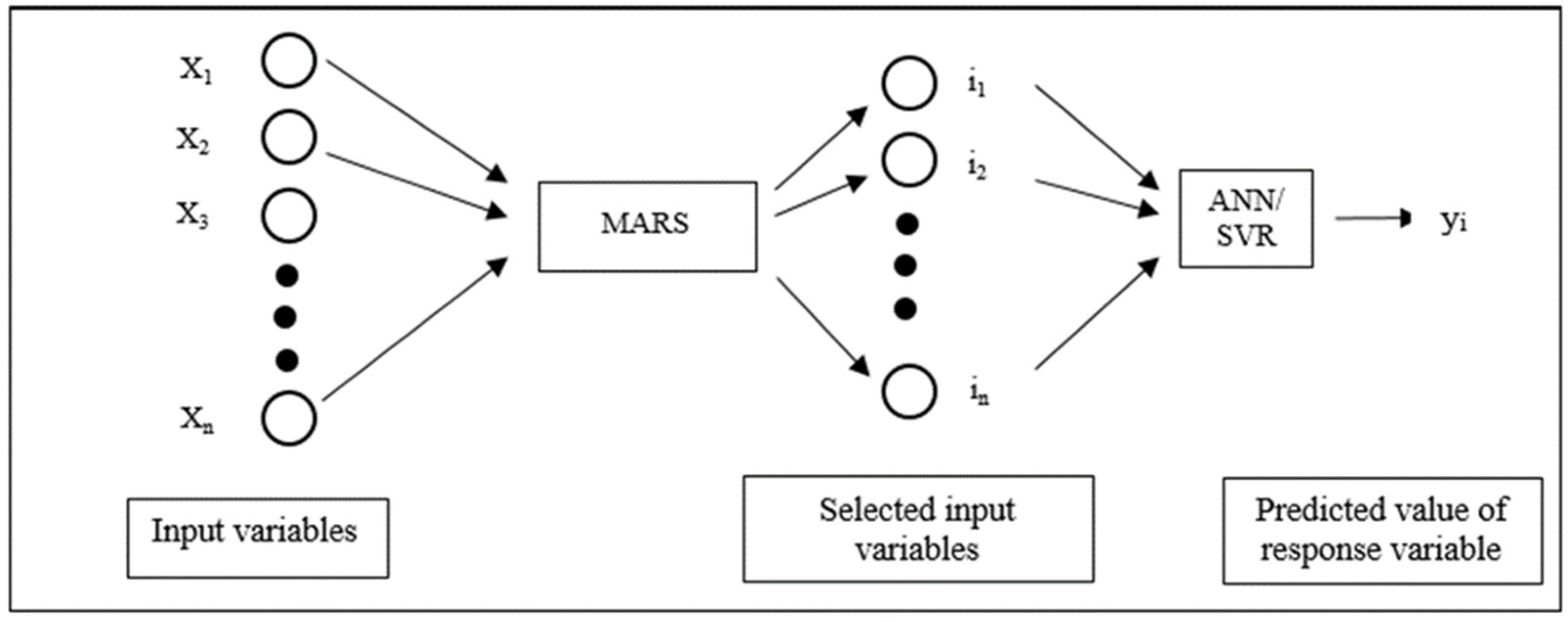
In the literature, most researchers have restricted themselves to using only one method such as ANN in their study. Comparative study and hybrid modelling of soft computing techniques with variable selection on particular datasets is yet to be done. This motivated the present comparative study of different soft computing techniques such as ANN, MARS and SVR. A hybrid model was formulated using MARS and ANN/SVR. These techniques and the proposed hybrid model were applied to the lentil dataset, and their modelling and forecasting performances were compared using different statistical measures. The remaining portion of the paper is divided into materials and methods, results and discussion, and a conclusion section.

2. Materials and Methods

2.1. Plant Material and Field Experiment

The experimental data for this study comprise 518 lentil accessions, of which 206 entries are exotic collections and 312 are indigenous collections, including 59 breeding lines. These accessions were grown in augmented block design with five checks during rabi season, 2006–07 at ICAR-Indian Institute of Pulses Research, Kanpur. Accessions were evaluated for 21 descriptors, including plant characteristics and seed characteristics following the biodiversity and national Distinctness, Uniformity and Stability (DUS) descriptors guidelines. More information on the descriptors is accessible in [36]. Ten numerical descriptors including days to 50% flowering (DF), plant height (PH), days to 90% maturity (DM), 100 seed weight (SW), biological yield per plant (BYP), number of primary branch per plant (PB), number of secondary branch per plant (SB), number of pods per plant (PPP), yield per plant (YPP) and plant height at lowest pod (PHLP) were used for detailed analysis. Our target variable was yield per plant (YPP), which was influenced by other factors (See Supplementary Materials).

2.2. Machine Learning Models

2.2.1. Multivariate Adaptive Regression Spline (MARS) Model

The MARS model for a dependent (outcome) variable y, and M terms, can be summarized in the following equation [37]:
y ^ = f ^ M ( X ) = c 0 + m = 1 M c m B m ( X )
where y ^ is the dependent variable (YPP) predicted by the MARS model, c0 is a constant, B m ( X ) is the mth basis function, which may be a single spline basis function, and c m is the coefficient of the mth basis function. Both the variables to be introduced into the model and the knot positions for each individual variable have to be optimized. For a dataset X containing n objects and p explanatory variables, there are N = n × p pairs of spline basis functions with knot locations (i = 1, 2, …, n; j = 1, 2, …, p). In the present study, x = 206 entries are exotic collections and 312 are indigenous collections, including 59 breeding lines, p = 9 and n = 518. MARS was used as a variable selection model in the present study.

2.2.2. Artificial Neural Network (ANN) Model

Artificial neural networks (ANNs) are nonlinear data-driven self-adaptive approaches as opposed to the traditional model-based methods [38]. ANNs have the ability to identify correlations between input variables and associated target values. ANNs can solve problems involving nonlinear and complicated data even if the data are noisy and inaccurate since they mimic the learning process of the human brain. They are therefore perfectly suited for modelling agricultural data, which are known to be complicated and frequently nonlinear.
The output of a neural network can be expressed by the following equation [39]:
y t = α 0 + j = 1 n α j f ( i = 1 m β i j y t 1 + β o j ) + ε t
where yt is output of neural network model (yield per plant); n is number of hidden nodes; m is the number of input nodes; f is the net input of the activation function; β i j {I = 1, 2, …, m; j = 0, 1, …, n} are the weights from input to hidden nodes; α j { j = 0 , 1 , , n } are the vectors of weights from hidden to output node; α 0 and β 0 j are the weights of arcs leading from bias terms. Activation function is a differentiable function that is used for smoothing the result of the cross product of the covariate or neurons and the weights. In artificial neural networks, the activation function of a node defines the output of that node given an input or set of inputs. In the present study, logistic function was used as activation function and the Levenberg–Marquardt (LM) learning algorithm was used to adjust the weights in the multi-layered feedforward networks.

2.2.3. Support Vector Regression (SVR) Model

Support Vector Machine (SVM) is nonlinear algorithms used in supervised learning frameworks for data analysis and pattern recognition [8]. The traditional support vector machine technique is the predecessor of the SVR that is a nonlinear prediction model. Based on Vapnik’s concept of support vectors [8], Drucker et al. [40] first introduced support vector regression. SVR’s primary objective is to maximize the difference between predicted and actual values while minimizing error by adding a hyperplane. The SVR model can be written as:
y = i = 1 N W i K e r ( x i , x j ) + b
where y is our dependent variable (YPP), Wi is associated weight and K e r ( x i , x j ) is the nonlinear mapping function known as kernel function for input (independent) variables x i  (I = 1, 2, …, 9).

2.2.4. Hyperparameter Tuning of Machine Learning Models

Hyperparameter is one of the important factors in the ML model’s accuracy and prediction. Hyperparameters work differently in different datasets [17,41]. Choosing the best hyperparameter values improves the stability of any ML performance. Randomly, a ratio of 80 and 20 of the whole dataset was used for the training sample and the testing sample, respectively. The k fold cross-validation method was adopted to deal with the model over fitting problem. The cross-validation method evaluates ML algorithms’ capacity to handle new and unexplored data. In this method, the dataset is divided into approximately k equal-sized groups (folds) at random. The data are trained on k-1 folds, with the first fold being treated as a testing set. For each dataset in this investigation, three folds (k = 3) were taken. Some studies [13,21,42,43] suggest the superiority of this approach for a small dataset. The details of used hyperparameters for the used ML models are provided in Table 1. The hyperparameter tuning was conducted based on the trial-and-error method for minimizing root mean square error (RMSE).

2.3. Proposed Mars Based Hybrid Model

In the present study, MARS-based hybrid models have been developed by combing them with ANN and SVR, respectively. The main motive to develop these hybrid models was to harness the variable selection ability of MARS algorithm and prediction ability of ANN/SVR simultaneously. First, MARS algorithm was used to find important variables among the independent variables that influences yield variable. Then these selected variables were taken as input variables to predict yield variable (Figure 1). The pictorial representation of the hybrid methodology can be summed up in the following steps:
  • Step 1. Start model building with all available predictors.
  • Step 2. Apply MARS algorithm for extracting the important predictors based on its importance.
  • Step 3. Build the machine learning model (ANN/SVR) using the selected predictors.
  • Step 4. Obtain prediction using the model obtained in Step 3.
Figure 1. MARS-based ANN/SVR hybrid framework.
Agriculture 13 00596 g001

2.4. Model Performance and Accuracy of Fitted Models

The model accuracy measures for root mean squared error (RMSE), mean absolute deviation (MAD), mean absolute percentage error (MAPE) and maximum error (ME) were used to select the best models. The formulas were used as follows:
R M S E = i = 1 N ( y i y ^ i ) 2 N M A D = i = 1 N y i y ^ i N M A P E = i = 1 N y i y ^ i y i N M E = max i = 1 N y i y ^ i
where y i and y ^ i are the actual value and predicted value of response variable and N is the number of data. The Diebold Mariano (DM) test [44] was used in addition to accuracy measurements to compare the final fitted models.

3. Results

In this study the MARS, ANN and SVR model was fitted with the help of R. Two new R packages i.e., “MARSANNhybrid” [45] and “MARSSVRhybrid” [46] were developed for fitting of the MARS-based ANN and SVR models, respectively. The hyperparameters of the fitted models are described in Table 1.

3.1. Data Processing and Statistical Analysis

The basic aim of model building is to find out the existence of a relationship between the output and input variables. The summary statistics such as mean, range, standard deviation and coefficient of variation (CV) of parameters were checked (Table 2). The lowest coefficient of variation was observed in DM character, while dependent YPP showed the highest variation. Among the independent variables, the highest variability was found in the number of pods per plant (PPP).
The correlation study of input variables with outcome was explored (Figure 1) for the aforementioned lentil dataset. The Pearson correlation coefficients of input variables with output variables helped to identify the plant characters (traits) that have a strong correlation with output. As per Figure 2, there is a significant positive correlation between yields per plant (YPP) and pods per plant (PPP); biological yield per plant (BYP); number of secondary branches per plant (SB); plant height at lowest pod (PHLP); number of primary branches per plant (PB); plant height (PH); and 100 seed weight (SW). In the literature, similar types of correlation results were reported by different researchers who showed that PH [42,47,48], PB and SB [42,47,48], PPP [42], SW [42], PHLP [42] and BYP [42] are closely related to the yield of lentil. We also found a significant negative correlation between YPP and days to 90% maturity (DM) and days to 50% flowering (DF). These negative relationships were confirmed by some researchers [42,49,50].
Figure 2 depicts the Pearson correlation coefficients of input variables with the yield per plant of lentil. Variables were normalized within ranges [0.1, 1] for fitting in the ML models [51]. The given below formula was used for normalization:
x n = x i x min x max x min
where xi is the original data, xn is the normalized values, and xmax and xmin are the maximum and minimum values, respectively. Denormalised has been done prior to calculation of performance measures.

3.2. Input Variable Selection

MARS was used as a variable selection method. MARS degree largely influences the performance of model fitting and forecasting. Hence, we critically examined the performance of the model on different degrees (df 1, 2 and 3). The performance for the MARS model of degree 1, 2 and 3 were evaluated. It was found that the model complexity increased as the MARS degree increased. To compare the model accuracy of these MARS models, RMSE, MAD, MAPE and ME were computed. Table 3 presents the RMSE, MAD, MAPE and ME of the three MARS models. It was found that the MARS model with interaction terms tended to perform better than the model without interaction (MARS model with degree 1). The MARS model with degree of 3 had smaller RMSE, MAD and MAPE values compared to the MARS model with degree of 1 and 2. Moreover, the performance of the MARS model with degree of 3 followed all the assumptions of model adequacy, while the other two models failed to satisfy those assumptions. Therefore, the MARS model with degree of 3 was selected for the model fitting. The selected equation of the MARS model is:
Y(YPP) = 1.85 − 8.43 × BF1 − 0.15 × BF2 + 0.03 × BF3 + 0.29 × BF4 + 4.06 × BF5 + 0.04 × BF6
−0.01 × BF7 + 0.01 × BF8 − 0.001 × BF9 + 0.002 × BF10 − 0.21 × BF11 − 0.0002 × BF12
On the basis of generalized cross-validation (GCV) and residual sum of squares (RSS), a MARS model of order 3 was built to extract the significant variables. In Table 4, the MARS model’s chosen variables are listed. The dependent variables were then predicted using the seven variables that were chosen.

3.3. ANN Model Development

For model-building purposes, we varied our model architecture with 1 to 5 hidden nodes with a single hidden layer. The resilient backpropagation method was used for model training. In the present study, neural network models were fitted with rep = 1 to 3, stepmax = 1 × 10⁵ to 1 × 10⁸ and threshold = 0.01. The schematic representation of the fitted ANN model with weights is shown in Figure 3. Table 5 summarizes the error rate and performance measures of fitted ANN with a different number of hidden nodes. The ANN model with 1, 2, 3 and 5 hidden nodes had the same performance. However, the ANN model with 4 hidden nodes gave the best result. Thus, the best-fitted replication in the ANN model with 4 hidden nodes was used for yield forecasting.

3.4. SVR Model Development

The SVR model was fitted using different types of kernel functions such as linear, radial basis, sigmoid and polynomial, although the most often used and recommended function is radial basis. However, it is recommended to select the appropriate kernel function for the given dataset. Therefore, SVR was fitted using the four different kernel basis functions, and the best model was selected on the basis of performance measures. Other significant hyperparameters in the SVR model, such as the epsilon factor, cross-validation and type of regression, also have a significant impact on the model’s performance. In Table 1, the values of these parameters that were used are reported. Tenfold cross-validation was used to validate the resulting model. Further, we focused our attention on selection of the appropriate kernel function. The support vectors produced using RBF, linear and polynomial were 323, 321 and 329, respectively. In the training phase, performance measures such as RMSE, MAD, MAPE and ME were computed for choosing the best forecasting model. From Table 6, it was observed that the SVR model with radial basis kernel function provided the best result on the basis of parsimonious representation. Hence, the SVR model with radial basis kernel function was employed for yield prediction.
Fit statistics values were used to examine the effectiveness of fitted models for both in-sample and out-of-sample predictions. In order to verify the model’s suitability, the specifics of the derived residuals were also examined. The value of the statistic of fitted models is shown in Table 7. It was found that MARS performed the best among the individual models, followed by SVR and ANN. To fit a local regression model to each sub-region, the MARS algorithm partitioned the dataset into a number of sub-regions. Redundancy of variables may cause overfitting problems in a single ANN (without MARS). Similar results in ANN were highlighted by researchers [30,31,32]. It might be the reason why the ANN performed poorly. The performance of a single SVR model was considerably affected by the same issues.
The out-of-sample performance of these hybrid models further demonstrates their strong generalizability. The DM test was also used to determine whether the MARS-ANN and MARS-SVR models were the best. The alternative MARS-ANN model outperformed the MARS-SVR model in terms of accuracy, which was the null hypothesis of the test. The significance of the Diebold–Mariano (DM) test is displayed in Table 8. The right-tailed DM test was used considering the models have equal accuracy. The test demonstrated the superiority of the MARS-ANN model over the MARS-SVR.

4. Discussion

The study revealed the superiority of proposed hybrid models for crop yield prediction. The results indicated that the proposed hybrid model had the power to capture the nonlinearity among the variables. The generic models such as ANN, SVR and MARS failed to capture the inherent data patterns and were unable to produce satisfactory prediction results. It is clear that variable selection provided extra advantages to the SVR and ANN models. Both of the proposed hybrid models outperformed their individual counterparts. It validated the advancements made by MARS in both the ANN and SVR models. As previously mentioned, key explanatory variables were retrieved with the aid of the MARS model in the case of hybrid models, and nonlinear forecasting techniques such as ANN and SVR were applied. The superior performance of the hybrid models may be attributable to parsimony and two-stage model construction. Further DM test results clarified MARS-ANN was the best model among the fitted models.

5. Conclusions

Modelling and forecasting of complex, multifactorial and nonlinear phenomenon such as crop yield have intrigued researchers for decades. This study is an attempt in the similar direction to contribute to the vast literature of crop-yield modelling. The study proposed novel hybrids based on MARS. The feature extraction ability of MARS was utilized, and efficient forecasting models were developed using ANN and SVR. The utility of the proposed models was illustrated and compared using a lentil dataset with baseline models. As these models do not depend on assumptions about functional form, probability distribution or smoothness and have been proven to be universal approximators.
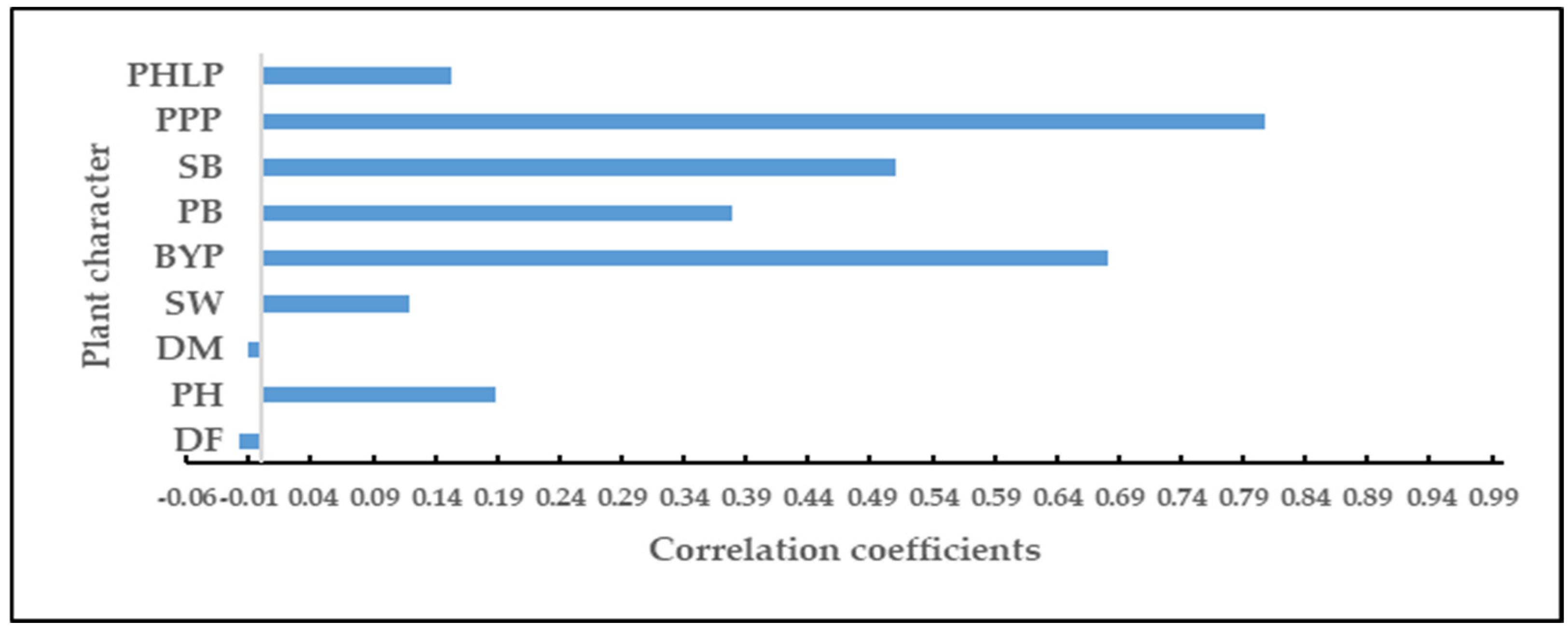
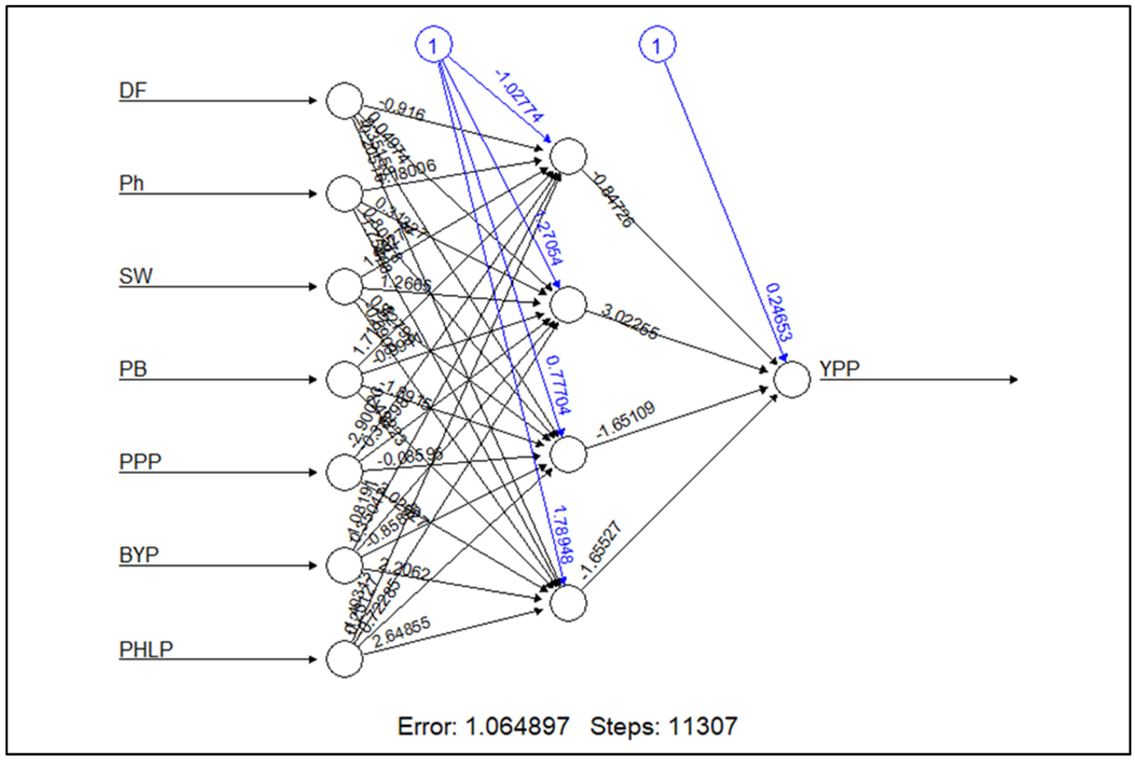
The novel hybrid model was built in two steps, each performing a specialized task. In the first step, important input variables were identified using the MARS model instead of hand-picking variables based on a theoretical framework. In the second step, nonlinear prediction techniques ANN and SVR were used for yield prediction using the selected variables. The performance of the models was compared using fit statistics such as RMSE, MAD, MAPE and ME. The proposed MARS-based hybrid models performed better as compared to the individual models such as MARS, SVR and ANN. This is largely due to the enhanced feature extraction capability of the MARS model coupled with the nonlinear adaptive learning feature of ANN and SVR. This proposed framework can be applied to a variety of datasets to capture the nonlinear relationship between independent and dependent variables. The R packages developed in this study have utility in multifactorial and multivariate experiments such as genomic selection, gene expression analysis, survival analysis, digital soil mappings, etc. Further, efforts can be directed to propose and evaluate hybrids of other soft computing techniques.

Supplementary Materials

The following are available online at https://www.mdpi.com/article/10.3390/agriculture13030596/s1. Supplementary sheet for Descriptors.

Author Contributions

P.D. conceived the conceptualization, investigation, formal analysis, data curation and writing original draft. G.K.J. gave the idea of conceptualization, resources, reviewing and editing. A.L. and R.P. performed supervision and edited the manuscript. All authors have read and agreed to the published version of the manuscript.

Funding

This research was funded by ICAR-Indian Agricultural Statistics Research Institute, New Delhi, India.

Institutional Review Board Statement

Not applicable.

Data Availability Statement

The data presented in this study are available on request from the corresponding author.

Acknowledgments

The authors are thankful to the Director, ICAR-IASRI for providing facilities for carrying out the present research.

Conflicts of Interest

The authors declare no conflict of interest.

References

  1. Sarker, A.; Erskine, W.; Singh, M. Regression models for lentil seed and straw yields in Near East. Agric. For. Meteorol. 2003, 116, 61–72. [Google Scholar] [CrossRef]
  2. Ghanem, M.E.; Marrou, H.; Soltani, A.; Kumar, S.; Sinclair, T.R. Lentil Variation in Phenology and Yield Evaluated with a Model. Agron. J. 2015, 107, 1967–1977. [Google Scholar] [CrossRef]
  3. Statistics Division (FAOSTAT), UN Food and Agriculture Organization, United Nations. Production of Lentils in 2020; Crops/World Regions/Production Quantity from Pick Lists; FAO: Rome, Italy, 2022. [Google Scholar]
  4. Mondal, M.M.A.; Puteh, A.B.; Malek, M.A.; Roy, S.; Yusop, M.R. Contribution of morpho-physiological traits on yield of lentil (Lens culinaris Medik). Aust. J. Crop Sci. 2013, 7, 1167–1172. Available online: http://www.cropj.com/mondal3506_7_8_2013_1167_1172.pdf (accessed on 10 September 2022).
  5. Muehlbauer, F.J. Seed Yield Components in Lentils. Crop Sci. 1974, 14, 403–406. [Google Scholar] [CrossRef]
  6. Seid, M. Crop Forecasting: Its Importance, Current Approaches, Ongoing Evolution and Organizational Aspects. FAO Report. 2016. Available online: https://www.fao.org/fileadmin/templates/rap/files/meetings/2016/160524_AMIS-CM_3.2.3_Crop_forecasting_Its_importance__current_approaches__ongoing_evolution_and.pdf (accessed on 1 April 2021).
  7. Alireza, B.B.; Mohamadreza, S.; Said, A.; Behnam, T.; Gafari, G. Path analysis of seed and oil yield in safflower. Commun. Plant Sci. 2012, 2, 15–20. Available online: https://cpsjournal.org/2012/04/09/path-analysis-safflower/ (accessed on 10 September 2022).
  8. Vapnik, V.N. Statistical Learning Theory, 1st ed.; Wiley-Interscience: New Delhi, India, 1998. [Google Scholar]
  9. Sarkar, S.; Ghosh, A.; Brahmachari, K.; Ray, K.; Nanda, M.K. Assessing the yield response of lentil (Lens culinaris Medikus) as influenced by different sowing dates and land situations in Indian Sundarbans. Legume Res.-Int. J. 2021, 44, 1203–1210. [Google Scholar] [CrossRef]
  10. Bagheri, A.; Zargarian, N.; Mondani, F.; Nosratti, I. Artificial neural network potential in yield prediction of lentil (Lens culinaris L.) influenced by weed interference. J. Plant Prot. Res. 2020, 60, 284–295. [Google Scholar] [CrossRef]
  11. Khairunniza-Bejo, S.; Mustaffha, S.; Ismail, W.I.W. Application of artificial neural network in predicting crop yield: A review. J. Food Sci. Eng. 2014, 4, 1–9. Available online: http://psasir.upm.edu.my/id/eprint/36505/1/Application%20of%20artificial%20neural%20network%20in%20predicting%20crop%20yield.pdf (accessed on 10 September 2022).
  12. Schultz, A.; Wieland, R. The use of neural networks in agroecological modelling. Comput. Electron. Agric. 1997, 18, 73–90. [Google Scholar] [CrossRef]
  13. Uno, Y.; Prasher, S.O.; Lacroix, R.; Goel, P.K.; Karimi, Y.; Viau, A.; Patel, R.M. Artificial neural networks to predict corn yield from Compact Airborne Spectrographic Imager data. Comput. Electron. Agric. 2009, 47, 149–161. [Google Scholar] [CrossRef]
  14. Lee, T.S.; Chen, I.F. A two-stage hybrid credit scoring model using artificial neural networks and multivariate adaptive regression splines. Expert Syst. Appl. 2005, 28, 743–752. [Google Scholar] [CrossRef]
  15. Zhang, W.; Goh, A.T.C. Multivariate adaptive regression splines and neural network models for prediction of pile drivability. Geosci. Front. 2016, 7, 45–52. [Google Scholar] [CrossRef] [Green Version]
  16. Khazaei, J.; Naghavi, M.R.; Jahansouz, M.R.; Salimi-Khorshidi, G. Yield estimation and clustering of chickpea genotypes using soft computing techniques. Agron. J. 2008, 100, 1077–1087. [Google Scholar] [CrossRef]
  17. Higgins, A.; Prestwidge, D.; Stirling, D.; Yost, J. Forecasting maturity of green peas: An application of neural networks. Comput. Electron. Agric. 2010, 70, 151–156. [Google Scholar] [CrossRef]
  18. Gandhi, N.; Petkar, O.; Armstrong, L.J.; Tripathy, A.K. Rice crop yield prediction in India using support vector machines. In Proceedings of the 2016 13th International Joint Conference on Computer Science and Software Engineering, JCSSE, Khon Kaen, Thailand, 13–15 July 2016. [Google Scholar] [CrossRef]
  19. Gopal, G.; Bagade, A.; Doijad, S.; Jawale, L. Path analysis studies in safflower germplasm (Carthamus tinctorius L.). Int. J. Curr. Microbiol. Appl. Sci. 2014, 3, 347–351. Available online: https://www.ijcmas.com/vol-3-12/G.R.Gopal,%20et%20al.pdf (accessed on 10 September 2022).
  20. Deo, R.C.; Kisi, O.; Singh, V.P. Drought forecasting in eastern Australia using multivariate adaptive regression spline, least square support vector machine and M5Tree model. Atmos. Res. 2017, 184, 149–175. [Google Scholar] [CrossRef] [Green Version]
  21. Su, Y.; Xu, H.; Yan, L. Support vector machine-based open crop model (SBOCM): Case of rice production in China. Saudi J. Biol. Sci. 2017, 24, 537–547. [Google Scholar] [CrossRef]
  22. Klompenburg, T.V.; Kassahun, A.; Catal, C. Crop yield prediction using machine learning: A systematic literature review. Comput. Electron. Agric. 2020, 177, 105709. [Google Scholar] [CrossRef]
  23. Batool, D.; Shahbaz, M.; Shahzad Asif, H.; Shaukat, K.; Alam, T.M.; Hameed, I.A.; Ramzan, Z.; Waheed, A.; Aljuaid, H.; Luo, S. A Hybrid Approach to Tea Crop Yield Prediction Using Simulation Models and Machine Learning. Plants 2022, 11, 1925. [Google Scholar] [CrossRef]
  24. Cubillas, J.J.; Ramos, M.I.; Jurado, J.M.; Feito, F.R. A Machine Learning Model for Early Prediction of Crop Yield, Nested in a Web Application in the Cloud: A Case Study in an Olive Grove in Southern Spain. Agriculture 2022, 12, 1345. [Google Scholar] [CrossRef]
  25. Bali, N.; Singla, A. Emerging trends in machine learning to predict crop yield and study its influential factors: A survey. Arch. Comput. Methods Eng. 2022, 29, 95–112. [Google Scholar] [CrossRef]
  26. Ji, Z.; Pan, Y.; Zhu, X.; Zhang, D.; Dai, J. Prediction of Corn Yield in the USA Corn Belt Using Satellite Data and Machine Learning: From an Evapotranspiration Perspective. Agriculture 2022, 12, 1263. [Google Scholar] [CrossRef]
  27. Bishop, M.C. Neural Networks for Pattern Recognition; Oxford University Press: New York, NY, USA, 1995. [Google Scholar]
  28. May, R.; Dandy, G.; Maier, H. Review of input variable selection methods for artificial neural networks. Artif. Neural Netw.–Methodol. Adv. Biomed. Appl. 2011, 10, 19–45. [Google Scholar]
  29. Montomery, D.C.; Peck, E.A.; Vining, G.G. Introduction to Linear Regression Analysis, 4th ed.; Wiley-Interscience: New Delhi, India, 2006. [Google Scholar]
  30. Cai, J.; Luo, J.; Wang, S.; Yang, S. Feature selection in machine learning: A new perspective. Neurocomputing 2018, 300, 70–79. [Google Scholar] [CrossRef]
  31. Pishgoo, B.; Azirani, A.A.; Raahemi, B. A dynamic feature selection and intelligent model serving for hybrid batch-stream processing. Knowl.-Based Syst. 2022, 256, 109749. [Google Scholar] [CrossRef]
  32. Zhao, S.; Wang, M.; Ma, S.; Cui, Q. A feature selection method via relevant-redundant weight. Expert Syst. Appl. 2022, 207, 117923. [Google Scholar] [CrossRef]
  33. Friedman, J.H. Multivariate adaptive regression splines. Ann. Stat. 1991, 19, 1–67. [Google Scholar] [CrossRef]
  34. Sekulic, S.; Kowalski, B.R. MARS: A tutorial. J. Chemom. 1992, 6, 199–216. [Google Scholar] [CrossRef]
  35. Lee, T.S.; Chiu, C.C.; Chou, Y.C.; Lu, C.J. Mining the customer credit using classification and regression tree and Multivariate adaptive regression splines. Comput. Stat. Data Anal. 2006, 50, 1113–1130. [Google Scholar] [CrossRef]
  36. Jha, G.K.; Chiranjit, M.; Jyoti, K.; Gajab, S. Nonlinear principal component based fuzzy clustering: A case study of lentil genotypes. Indian J. Genet. Plant Breed. 2014, 74, 189–196. Available online: http://isgpb.co.in (accessed on 1 April 2021). [CrossRef]
  37. Friedman, J.H.; Roosen, C.B. An introduction to multivariate adaptive regression splines. Stat. Methods Med. Res. 1995, 4, 197–217. [Google Scholar] [CrossRef]
  38. Jha, G.K.; Sinha, K. Time-delay neural networks for time series prediction: An application to the monthly wholesale price of oilseeds in India. Neural. Comput. Appl. 2014, 3–4, 563–571. [Google Scholar] [CrossRef]
  39. ASCE Task Committee on Application of Artificial Neural Networks in Hydrology. Artificial Neural Networks in Hydrology. I: Preliminary Concepts. J. Hydrol. Eng. 2000, 5, 115–123. [Google Scholar] [CrossRef]
  40. Drucker, H.; Surges, C.J.C.; Kaufman, L.; Smola, A.; Vapnik, V. Support vector regression machines. Adv. Neural. Inf. Process. Syst. 1997, 9, 155–161. Available online: https://papers.nips.cc/paper/1996/file/d38901788c533e8286cb6400b40b386d-Paper.pdf (accessed on 1 April 2021).
  41. Abdipour, M.; Younessi-Hmazekhanlu, M.; Ramazani, M.Y.H.; Omidi, A.H. Artificial neural networks and multiple linear regression as potential methods for modeling seed yield of safflower (Carthamus tinctorius L.). Ind. Crops Prod. 2019, 27, 185–194. [Google Scholar] [CrossRef]
  42. Zhang, Q.M.; Zhang, G.P. Trend time series modeling and forecasting with neural networks. IEEE Trans. Neural Netw. 2008, 19, 808–816. [Google Scholar] [CrossRef]
  43. Diebold, F.X.; Mariano, R.S. Comparing predictive accuracy. J. Bus. Econ. Stat. 2002, 20, 134–144. [Google Scholar] [CrossRef]
  44. Das, P.; Lama, A.; Jha, G.K. MARSANNhybrid: MARS Based ANN Hybrid Model. 2021. Available online: https://CRAN.R-project.org/package=MARSANNhybrid (accessed on 1 April 2021).
  45. Das, P.; Lama, A.; Jha, G.K. MARSSVRhybrid: MARS SVR Hybrid. 2021. Available online: https://CRAN.R-project.org/package=MARSSVRhybrid (accessed on 1 April 2021).
  46. Lotfi, P.; Mohammadi-Nejad, G.; Golkar, P. Evaluation of drought tolerance in different genotypes of the safflower (Carthamus tinctorius L.). Iran. J. Agric. Sci. 2012, 5, 1–14. Available online: http://www.ijabbr.com (accessed on 1 April 2021).
  47. Yang, Y.-X.; Wu, W.; Zheng, Y.-L.; Huang, C.-Y.; Liu, R.-J.; Chen, L. Correlation and path analysis on characters related to flower yield per plant of Carthamus tinctorius. Zhong Cao Yao 2006, 37, 105. Available online: https://pesquisa.bvsalud.org/portal/resource/pt/wpr-574547 (accessed on 1 April 2021).
  48. Khalili, M.; Pour Aboughadareh, A.; Naghavi, M.R.; Naseri Rad, H. Path analysis of the relationships between seed yield and some of morphological traits in safflower (Carthamus tinctorius L.) under normal irrigated and rainfed conditions. Tech. J. Eng. Appl. Sci. 2014, 3, 1692–1696. Available online: http://www.tjeas.com (accessed on 1 April 2021).
  49. Senobari, S.; Sabzalian, M.R.; Saeidi, G. Evaluation of phenotypic and genetic relationships between agronomic traits, grain yield and its components in genotypes derived from interspecific hybridization between wild and cultivated safflower. Iran. J. Field Crop. Sci. 2016, 47, 131–139. Available online: https://www.cabdirect.org/cabdirect/abstract/20163237386 (accessed on 1 April 2021).
  50. Haykin, S. Neural Networks: A Comprehensive Foundation; Prentice Hall: Toronto, ON, Canada, 1999. [Google Scholar]
  51. Das, P. Study on Machine Learning Techniques Based Hybrid Model for Forecasting in Agriculture. Ph.D. Thesis, Indian Agricultural Research Institute, New Delhi, India, 2020. Available online: http://krishikosh.egranth.ac.in/handle/1/5810147805 (accessed on 1 April 2021).
Figure 2. Pearson correlation coefficients of input variables with yield per plant of lentil.
Agriculture 13 00596 g002
Figure 3. Schematic diagram of fitted neural network structure.
Agriculture 13 00596 g003
Table 1. Hyper parameter tuning of the machine learning model.
ModelHyper Parameters
ANNTraining algorithmResilient back propagation (Rprop)
Maximum steps up to which the neural network is trained (Stepmax)1 × 10⁷
The number of repetitions used to train the neural network model (Rep)3
Threshold (threshold value of the partial derivatives of the error function)0.01
SVRDefining algorithmsKernel
Regularization parameter (C)1
Kernel coefficient (Gamma)Scale
Penalty function (Epsilon)0.1
Cross validation10
MARSNumber of model terms upper bound (Nmax)20
Penalty coefficient (b)3
Table 2. Summary of the parameters of lentil.
ParameterRangeMeanStandard DeviationCV
DF58–10678.6910.7513.66
PH17–47.630.794.7915.55
DM114–140126.034.703.72
SW1.2–4.12.430.5321.75
BYP4.2–2813.373.7528.01
PB2–93.761.0628.20
SB4–1810.222.3923.40
PPP3.7–309.3116.1647.5340.92
YPP0.2–10.73.721.6143.25
PHLP1–1910.742.3021.44
Table 3. Performance measures for different MARS models.
DegreeRMSEMADMAPE
10.59720.51340.1792
20.44920.48660.1566
30.43560.48420.1565
Table 4. Predictor importance for MARS with degree of 3.
VariableGCVRSS
PPP100100
SW46.548.6
Ph31.233.9
BYP31.133.9
PHLP25.528
PB18.420.1
DF6.67.9
Table 5. Performance measures for different number of nodes in ANN models.
No. of Nodes in Hidden LayerRMSEMADMAPE
11.61341.21690.4612
21.61341.21690.4612
31.61341.21690.4612
40.96270.62880.1828
51.15121.01910.3521
Table 6. Performance measures for different kernel function in SVM.
Kernel FunctionRMSEMAD
Radial basis0.64740.3602
Linear0.85990.5231
Polynomial0.8270.5253
Sigmoid0.82690.5253
Table 7. Performance measures for different fitted models.
ModelRMSEMADMAPEME
In-sampleANN0.98270.62880.18288.1055
MARS0.43560.48420.15654.2157
MARS-ANN0.08020.06070.24780.3918
MARS-SVR0.08260.05790.18340.8498
MLR0.98690.65200.18409.10
SVR0.64740.36020.10897.1265
Out-sampleANN0.81420.64350.23082.4871
MARS0.94150.61470.27695.3540
MARS-ANN0.08020.05790.22140.7085
MARS-SVR0.06580.05790.16260.2206
MLR0.85200.06100.28523.6302
SVR0.68530.49020.27072.6435
Table 8. Results of DM test of compared models.
ModelDM Valuep ValueRemarks
MARS-ANN vs. MARS-SVR4.185<0.01The accuracy of MARS-ANN is better than MARS-SVR.
MARS-ANN vs. ANN5.304<0.01The accuracy of MARS-ANN is better than ANN model.
MARS-ANN vs. MARS5.725<0.01The accuracy of MARS-ANN is better than MARS model.
MARS-ANN vs. SVR5.955<0.01The accuracy of MARS-ANN is better than SVR model.
MARS-SVR vs. ANN6.563<0.01The accuracy of MARS-SVR is better than ANN model.
MARS-SVR vs. SVR6.823<0.01The accuracy of MARS-SVR is better than SVR model.
MARS-SVR vs. MARS6.235<0.01The accuracy of MARS-SVR is better than MARS model.
Disclaimer/Publisher’s Note: The statements, opinions and data contained in all publications are solely those of the individual author(s) and contributor(s) and not of MDPI and/or the editor(s). MDPI and/or the editor(s) disclaim responsibility for any injury to people or property resulting from any ideas, methods, instructions or products referred to in the content.

