

Automation of Crop Disease Detection through Conventional Machine Learning and Deep Transfer Learning Approaches


Abstract
1. Introduction
Related Work
2. Materials and Methods
2.1. Dataset
2.2. Experimental Setup
2.3. Machine Learning Approach
2.3.1. Image Preprocessing
2.3.2. Background Removal and Segmentation of the Diseased Region
2.3.3. Feature Extraction

| Angular Second Moment | It denotes the summation of the squares in the grey-level co-occurrence matrix. |
| Contrast | It represents the local intensity difference sum, where i ≠ j. |
| Correlation | It denotes the gray-level linear dependence of adjacent pixels. |
| Squares Sum | Variance |
| Sum Mean (μ) | |
| Inverse Different Moment | |
| Sum Variance | |
| Sum Entropy | |
| Entropy | It indicates the required amount of information on the image for compression. |
| Difference Variance | |
| Difference Entropy | |
| Correlation information measures | |
| where: HXY = − | |
| Furthermore, HX and HY are the (is the marginal likelihood matrix entry obtained by adding the rows) and (stands for the marginal likelihood matrix entry obtained by adding the columns) entropies. | |
| Maximal Correlation Coefficient |
2.3.4. Classification
| Polynomial kernel function | |
| The outcome is a polynomial classifier of the rank q | |
| Radial Basis Kernel (RBF) function | |
| Sigmoid kernel function |
2.4. Deep Learning Approach
2.4.1. Image Preprocessing
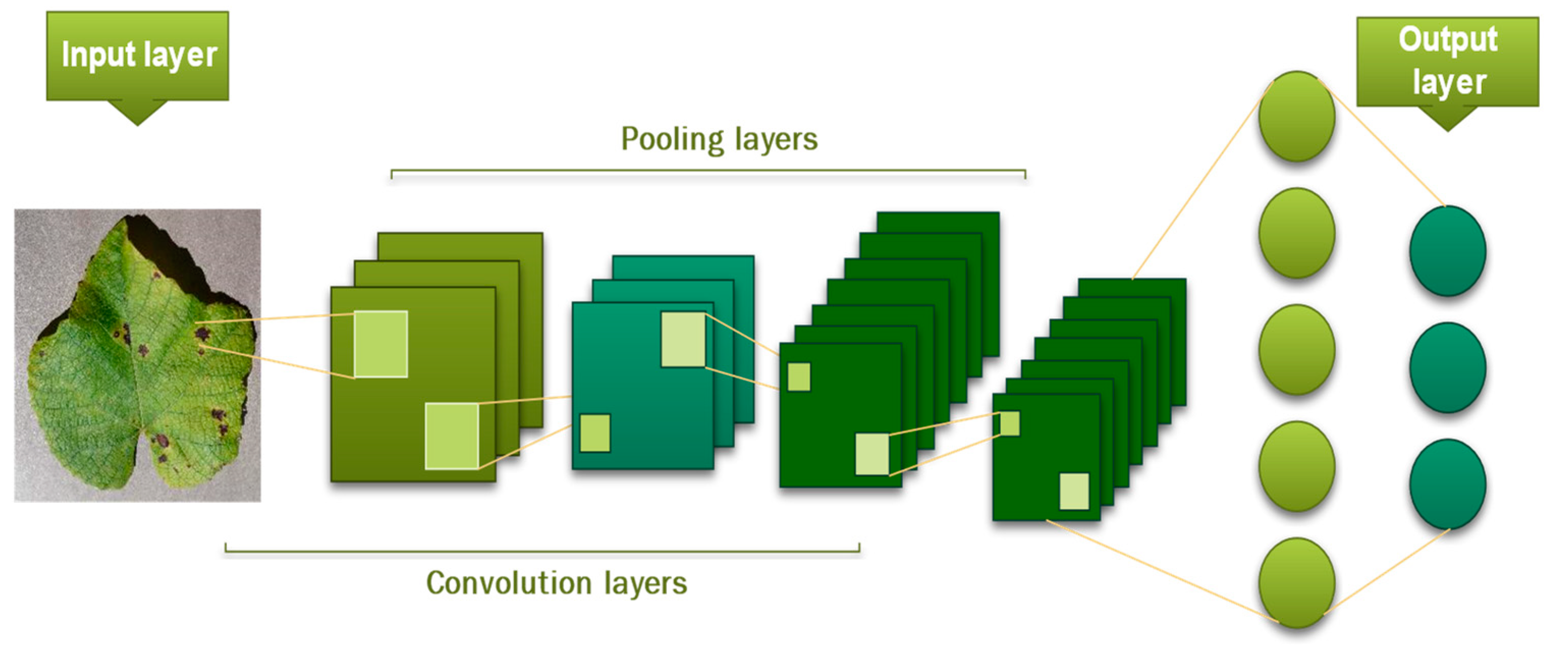
2.4.2. Convolutional Neural Networks CNN
- − To hold the output restricted to the desired range.
- − To encompass a non-linear functionality in the data.
Different Kinds of Activation Functions
| Activation Function | Advantages | Disadvantages | When Might It Be Used? |
|---|---|---|---|
| Sigmoid [41] | -Smooth gradient, avoiding “skips” in the output values -Consistently differentiable | -Decreasing gradient: It refuses to learn more and is quite slow to reach an accurate prediction. -Computationally demanding | If the output lies between (0,1) then the sigmoid may be employed |
| Tanh [41] | -Centered on zero -Continuously differentiable at any point | -Vanishing gradient issue -Since the function is nonlinear, it can effortlessly backpropagate errors/faults | If the output lies between (0,1) or (−1, 1), then the tanh can be used |
| ReLU [41] | -It is computationally efficient and allows the net to get together quickly -Backpropagation is allowable -Non-linear: Although it possesses a derivative function | -Once the inputs contact zero/negative, the gradient becomes zero, making the network unable to perform backpropagation and failing at learning -Unlimited and undifferentiable at zero | ReLU is widely used, when we want to predict output values higher than 1 because tanh or sigmoid are not appropriate for this purpose |
| Softmax [39] | -Proficient in managing different classes, single class among other functions -Provides the probability of the input value to be in a particular class. | -Does not consider the rejection of null values -This is unlikely to work if data are non-linearly separable | when predicting a probability for a multi-class task, the Softmax function must be implemented in the last layer |
| Softplus [41] | -Soft derivative employed in backpropagation and it is equivalent to a sigmoid function | -Operation not as affordable as ReLU | Rather never |
| Softsign [41] | -Better and faster learning due to the absence of difficulties related to the vanishing gradient -Softsign prevents neuron saturation, which enables much more efficient learning. | -Frequently, the gradient yields either an extremely high or low value -More costly to calculate than tanh | Rather never |
| Swish [42] | -It yields an efficient propagation of information during training and has an improved accuracy as it is devoid of leakage gradient problems | -It is very costly in terms of calculation. | It is used in very deep networks, when the number of hidden layers is high (nearly 30) |
| LeakyReLU [42] | -Seeks to overcome the “dead neuron” -Straightforward implementation and low-cost operation | -Large gradients can change the weights so that neural units are permanently disabled (never activated). | To be used only if you expect a “dying ReLU” problem, so it should be applied in hidden layers. |
| ELU [44] | -It can deliver negative outputs -Resolves both the vanishing gradient and the dying ReLU problem | -Computationally demanding -For x 0, it can jump the activation along with the output range of [0, ] | When the risk of overfitting is high, and it should be used in hidden layers. |
Optimization Method
Optimizer Training Specifications
| Optimizers | Specifications |
|---|---|
| SGD [47] | -weight decay = 0.0005, momentum = 0.9, nesterov = False, lr = 0.001 |
| Adagrad [48] | -epsilon = 1 × 10⁻⁷, lr = 0.001 |
| RMSProp [49,56] | -epsilon = 1 × 10⁻⁷, rho = 0.9, lr = 0.001 |
| Adadelta [50] | -epsilon = 1 × , lr = 0.001, beta1 = 0.9, beta2 = 0.999, amsgrad = False |
| Adam [51] | -epsilon = 1 × , beta1 = 0.9, beta2 = 0.999, lr = 0.002 |
Hyperparameter Tunning
2.4.3. ResNet50
- DL Optimizer: Stochastic Gradient Descent (SGD).
- Shear range: 0.2.
- Activation function: ReLu/Sigmoid.
- Loss function: Binary-cross-entropy.
- The number of epochs: 100.
2.4.4. InceptionV3
- DL Optimizer: Adam
- Shear range: 0.2
- Activation function: Sigmoid
- Loss function: Binary-cross-entropy
- Number of epochs: 100
2.4.5. VGG16
- DL Optimizer: RMS prop.
- Shear range: 0.2.
- Activation function: Sigmoid.
- Loss function: Categorical-cross-entropy.
- Number of epochs: 100.
2.4.6. VGG19
- Optimizer: RMS prop.
- Shear range: 0.2
- Activation function: Sigmoid.
- Loss function: Binary-cross-entropy.
- Number of epochs: 100.
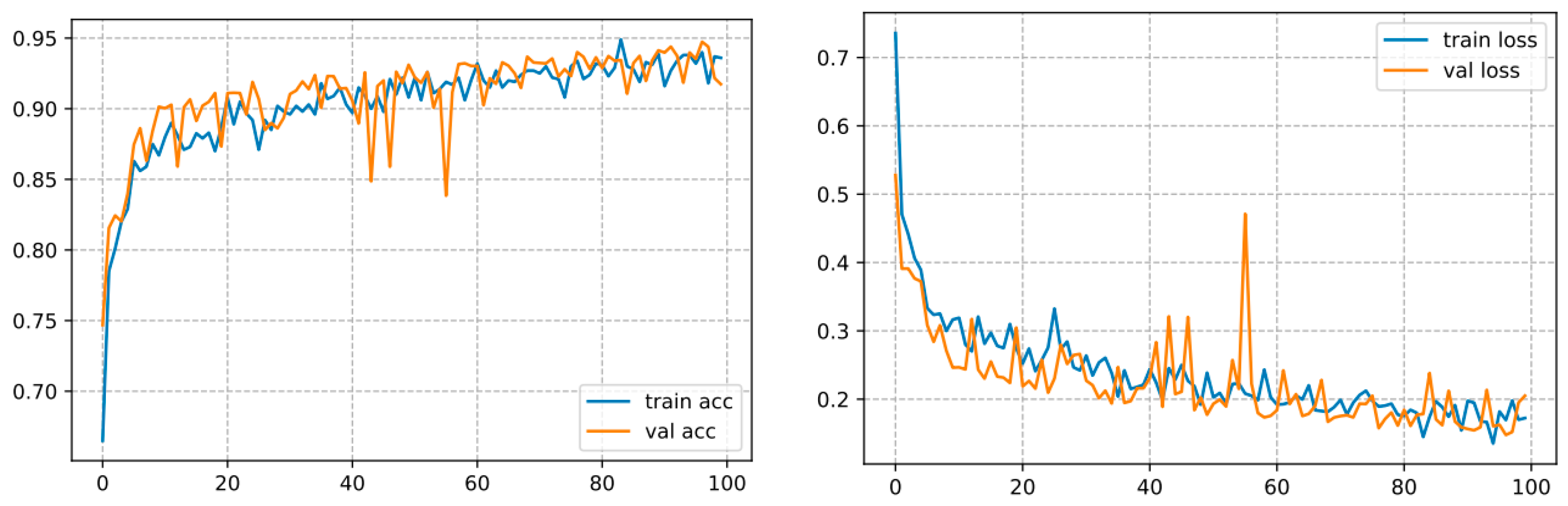
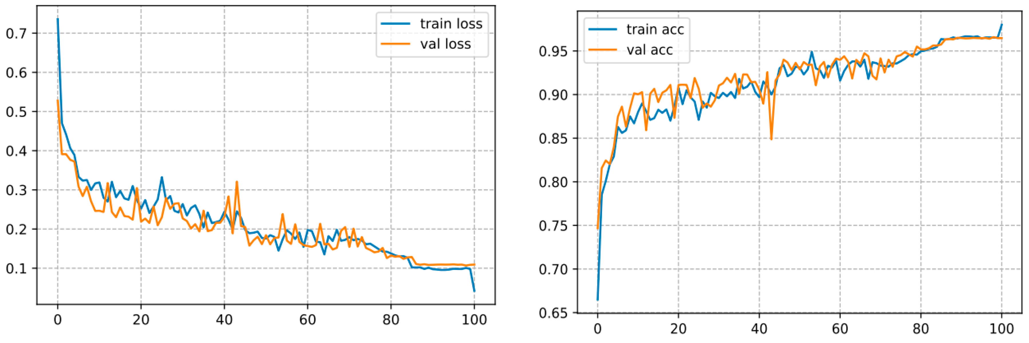
3. Experimental Results
3.1. Performance Measures
- Precision: It depicts in binary classifications all the positive classes predicted correctly by the model; how many of them are positive. It is computed by dividing the number of correctly classified positive samples by the number of predicted positive examples. The formula is expressed as follows:
- b.
- Recall/or sensitivity [61]: It sets the number of correctly predicted samples among all the positive classes. The equation is stated as below:
- c.
- F1-score [62]: The F1 score yields a global estimate of a test subject’s recall and accuracy. It refers to the harmonic average of recall and precision. Formally, the F1 score is determined by the following:
- d.
- Accuracy: This is a metric for assessing classification models. It is a fraction of all correct predictions. Formally, it is expressed as below:
- e.
- The confusion or error matrix [63]: It describes the classifier’s performance on the test data. It helps to identify and pinpoint each cluster that might have been misclassified by the classifier and to further improve the proposed classification model in the future. Each row represents the predicted class examples, and each column of the matrix represents the actual class examples. Thus, we computed the confusion matrix of each model to compare the different algorithms, as it allows us to measure the degree of classification model accuracy for each category. As we are dealing with a binary classification of leaf disease, we are interested in false negatives (FN). This is also called “type 2 error”, which represents the rate of misclassified crop leaves that appear healthy but are affected by diseases, thereby presenting a severe threat to the crop, especially if it concerns a viral disease that will spread swiftly over the field. To gain clearer perspective of classification findings, we employed confusion matrix plots and ROC curves (receiver operator characteristic) to depict the distinct crop binary classification results with distinct ML and DL algorithms.
- f.
- The ROC curve (Receiver Operating Characteristics Curve) [64] is a powerful tool for evaluating the performance of an ML/DL model. The ROC is applied to binary classification tasks where the output is composed of two distinct classes, and it represents a probability curve plotting the TPR against FPR at different threshold values and basically separates “signal” from “noise”. Otherwise, it expresses sensitivity as a function of 1- specificity for all possible threshold values of the marker studied. So, it demonstrates a trade-off phenomenon between specificity and sensitivity. Indeed, Sensitivity is the ability of the test to detect diseased leaves correctly, and specificity is the capacity of the test to detect healthy leaves correctly. This underscores the affectability of the classifier model. Where False Positive Rate (FPR) indicates the ratio of the negative class that was incorrectly classified by the classifier. Formally, it is expressed as below:where True Positive Rate (TPR) indicates the proportion of the positive class that was properly classified by the classifier. It is formally stated as follows:
- -
- When AUC = 0.5, the classifier is unable to differentiate between positive and negative class points. This means that it predicts a random or a steady class for all data points.
- -
- When 0.5 < AUC < 1, it is likely that the classifier can discriminate positive class values from negative ones. This stems from the ability of the classifier to detect a greater number of true negatives and true positives than false negatives and false positives.
3.2. Improvement in Classification Outcomes by DL Optimizers
3.3. Effectiveness of Deep Learning with Different Activation Functions
3.4. Computational Time Spent for Building Each Model
4. Discussion
Limitations of Machine Learning and Deep Learning
5. Conclusions
Author Contributions
Funding
Institutional Review Board Statement
Informed Consent Statement
Data Availability Statement
Conflicts of Interest
Abbreviations
| AI | Artificial Intelligence |
| AF | Activation function |
| ANN | Artificial Neural Networks |
| AUC | Area Under Curve |
| Adam | Adaptive moment estimation method |
| CA | Classification Accuracy |
| CA | Channel-wise Attention |
| CART | Classification And Regression Trees |
| CNN | Convolutional Neural Networks |
| DL | Deep Learning |
| ELM | Extreme Learning Machine |
| ELU | Exponential Linear Unit |
| FLS | Few-Short learning |
| FC | Fully Connected |
| IMPS | Importance Sampling |
| KNN | K-Nearest Neighbor |
| LDA | Latent Dirichlet Allocation |
| ML | Machine Learning |
| MLP | Multilayer Perceptron |
| NB | Naive Bayes |
| NN | Neural Networks |
| ResNet | Residual Network |
| ReLU | Rectified Linear Unit |
| RNN | Recurrent Neural Network |
| RF | Random Forest |
| ROS | Random Over Sampling |
| ROC | Receiver Operating Characteristics |
| RUS | Random Under Sampling |
| SGD | Stochastic Gradient Descent |
| SMOTE | Synthetic Minority Over-sampling Technique |
| SNN | Spiking Neural Networks |
| SVM | Support Vector Machine |
| TPMD | Tomato Powdery Mildew Disease |
| VGG | Visual Geometry Group |
References
- Savary, S.; Willocquet, L.; Pethybridge, S.J.; Esker, P.; McRoberts, N.; Nelson, A. The global burden of pathogens and pests on major food crops. Nat. Ecol. Evol. 2019, 3, 430–439. [Google Scholar] [CrossRef] [PubMed]
- Dhingra, G.; Kumar, V.; Joshi, H.D. Study of digital image processing techniques for leaf disease detection and classification. Multimedia Tools Appl. 2018, 77, 19951–20000. [Google Scholar] [CrossRef]
- Singh, V.; Sharma, N.; Singh, S. A review of imaging techniques for plant disease detection. Artif. Intell. Agric. 2020, 4, 229–242. [Google Scholar] [CrossRef]
- Mojjada, R.K.; Kumar, K.K.; Yadav, A.; Prasad, B.S.V. WITHDRAWN: Detection of plant leaf disease using digital image processing. Mater. Today Proc. 2020. [Google Scholar] [CrossRef]
- Vishnoi, V.K.; Kumar, K.; Kumar, B. Plant disease detection using computational intelligence and image processing. J. Plant Dis. Prot. 2021, 128, 19–53. [Google Scholar] [CrossRef]
- Applalanaidu, M.V.; Kumaravelan, G. A Review of Machine Learning Approaches in Plant Leaf Disease Detection and Classification. In Proceedings of the 2021 Third International Conference on Intelligent Communication Technologies and Virtual Mobile Networks (ICICV), Tirunelveli, India, 4–6 February 2021. [Google Scholar]
- Prathusha, P.; Murthy, K.; Srinivas, K. Plant Disease Detection Using Machine Learning Algorithms. In International Conference on Computational and Bio Engineering; Springer International Publishing: Berlin/Heidelberg, Germany, 2019. [Google Scholar]
- Pradhan, S.S.; Patil, R. Comparison of Deep Learning Approaches for Plant Disease Detection. In Proceedings of International Conference on Wireless Communication; Springer: Singapore, 2020. [Google Scholar] [CrossRef]
- Sachdeva, G.; Singh, P.; Kaur, P. Plant leaf disease classification using deep Convolutional neural network with Bayesian learning. Mater. Today Proc. 2021, 45, 5584–5590. [Google Scholar] [CrossRef]
- Devaraj, A.; Rathan, K.; Jaahnavi, S.; Indira, K. Identification of plant disease using image processing technique. In Proceedings of the 2019 International Conference on Communication and Signal Processing (ICCSP), Chennai, India, 4–6 April 2019. [Google Scholar]
- Iniyan, S.; Jebakumar, R.; Mangalraj, P.; Mohit, M.; Nanda, A. Plant Disease Identification and Detection Using Support Vector Machines and Artificial Neural Networks. In Artificial Intelligence and Evolutionary Computations in Engineering Systems; Springer: Berlin/Heidelberg, Germany, 2020; pp. 15–27. [Google Scholar] [CrossRef]
- Orchi, H.; Sadik, M.; Khaldoun, M. A General Survey on Plants Disease Detection Using Image Processing, Deep Transfer Learning and Machine Learning Techniques. In International Symposium on Ubiquitous Networking; Springer: Cham, Switzerland, 2021; pp. 210–224. [Google Scholar] [CrossRef]
- Argüeso, D.; Picon, A.; Irusta, U.; Medela, A.; San-Emeterio, M.G.; Bereciartua, A.; Alvarez-Gila, A. Few-Shot Learning approach for plant disease classification using images taken in the field. Comput. Electron. Agric. 2020, 175, 105542. [Google Scholar] [CrossRef]
- Pantazi, X.; Moshou, D.; Tamouridou, A. Automated leaf disease detection in different crop species through image features analysis and One Class Classifiers. Comput. Electron. Agric. 2019, 156, 96–104. [Google Scholar] [CrossRef]
- Arora, J.; Agrawal, U.; Sharma, P. Classification of Maize leaf diseases from healthy leaves using Deep Forest. J. Artif. Intell. Syst. 2020, 2, 14–26. [Google Scholar] [CrossRef]
- Tang, Z.; Yang, J.; Li, Z.; Qi, F. Grape disease image classification based on lightweight convolution neural networks and channelwise attention. Comput. Electron. Agric. 2020, 178, 105735. [Google Scholar] [CrossRef]
- Bhatia, A.; Chug, A.; Singh, A.P. Application of extreme learning machine in plant disease prediction for highly imbalanced dataset. J. Stat. Manag. Syst. 2020, 23, 1059–1068. [Google Scholar] [CrossRef]
- Shamsudin, H.; Yusof, U.K.; Jayalakshmi, A.; Khalid, M.N.A. Combining oversampling and undersampling techniques for imbalanced classification: A comparative study using credit card fraudulent transaction dataset. In Proceedings of the 2020 IEEE 16th International Conference on Control & Automation (ICCA), Singapore, 9–11 October 2020. [Google Scholar] [CrossRef]
- Chawla, N.V.; Bowyer, K.W.; Hall, L.O.; Kegelmeyer, W.P. SMOTE: Synthetic Minority Over-sampling Technique. J. Artif. Intell. Res. 2002, 16, 321–357. [Google Scholar] [CrossRef]
- Faust, J.; Hanelt, P.H.P.; Bhat, S.A. PlantVillage Dataset: A Dataset of 5539 Training and Validation Images for 26 Crop Species. 2016. Available online: https://www.plantvillage.org/ (accessed on 20 October 2022).
- Carneiro, T.; Da Nobrega, R.V.M.; Nepomuceno, T.; Bian, G.-B.; De Albuquerque, V.H.C.; Filho, P.P.R. Performance Analysis of Google Colaboratory as a Tool for Accelerating Deep Learning Applications. IEEE Access 2018, 6, 61677–61685. [Google Scholar] [CrossRef]
- Lukic, M.; Tuba, E.; Tuba, M. Leaf recognition algorithm using support vector machine with Hu moments and local binary patterns. In Proceedings of the 2017 IEEE 15th International Symposium on Applied Machine Intelligence and Informatics (SAMI), Herl’any, Slovakia, 26–28 January 2017; pp. 000485–000490. [Google Scholar] [CrossRef]
- Hu, M.-K. Visual pattern recognition by moment invariants. IEEE Trans. Inf. Theory 1962, 8, 179–187. [Google Scholar] [CrossRef]
- Basavaiah, J.; Anthony, A.A. Tomato Leaf Disease Classification using Multiple Feature Extraction Techniques. Wirel. Pers. Commun. 2020, 115, 633–651. [Google Scholar] [CrossRef]
- Karthickmanoj, R.; Sasilatha, T.; Padmapriya, J. Automated machine learning based plant stress detection system. Mater. Today Proc. 2021, 47, 1887–1891. [Google Scholar] [CrossRef]
- Haralick, R.M.; Shanmugam, K.; Dinstein, I.H. Textural Features for Image Classification. IEEE Trans. Syst. Man Cybern. 1973, SMC-3, 610–621. [Google Scholar] [CrossRef]
- Bankar, S.; Dube, A.; Kadam, P.; Deokule, S. Plant disease detection techniques using canny edge detection & color histogram in image processing. Int. J. Comput. Sci. Inf. Technol 2014, 5, 1165–1168. [Google Scholar]
- Koranne, S. Hierarchical data format 5: HDF5. In Handbook of Open Source Tools; Springer: Berlin/Heidelberg, Germany, 2011; pp. 191–200. [Google Scholar]
- Cortes, C.; Vapnik, V. Support-vector networks. Mach. Learn. 1995, 20, 273–297. [Google Scholar] [CrossRef]
- Hsu, W.-C.; Lin, L.-F.; Chou, C.-W.; Hsiao, Y.-T.; Liu, Y.-H. EEG Classification of Imaginary Lower Limb Stepping Movements Based on Fuzzy Support Vector Machine with Kernel-Induced Membership Function. Int. J. Fuzzy Syst. 2017, 19, 566–579. [Google Scholar] [CrossRef]
- Cunningham, P.; Delany, S.J. k-Nearest Neighbour Classifiers—A Tutorial. ACM Comput. Surv. 2021, 54, 1–25. [Google Scholar] [CrossRef]
- Liu, Y.; Wang, Y.; Zhang, J. New machine learning algorithm: Random forest. In International Conference on Information Computing and Applications; Springer: Berlin/Heidelberg, Germany, 2012; pp. 246–252. [Google Scholar]
- Breiman, L. Random forests. Mach. Learn. 2001, 45, 5–32. [Google Scholar] [CrossRef]
- Rish, I. An empirical study of the naive Bayes classifier. In IJCAI 2001 Workshop on Empirical Methods in Artificial Intelligence; IBM Research: New York, NY, USA, 2001; pp. 41–46. [Google Scholar]
- Blei, D.M.; Ng, A.Y.; Jordan, M.I. Latent dirichlet allocation. J. Mach. Learn. Res. 2003, 3, 993–1022. [Google Scholar]
- Trendowicz, A.; Jeffery, R. Classification and regression trees. In Software Project Effort Estimation; Springer: Berlin/Heidelberg, Germany, 2014; pp. 295–304. [Google Scholar]
- LeCun, Y.; Bengio, Y.; Hinton, G. Deep Learning. Nature 2015, 521, 436–444. [Google Scholar] [CrossRef]
- Schmidhuber, J. Deep Learning in Neural Networks: An Overview. Neural Netw. 2015, 61, 85–117. [Google Scholar] [CrossRef]
- Mercioni, M.A.; Holban, S. The most used activation functions: Classic versus current. In Proceedings of the 2020 International Conference on Development and Application Systems (DAS), Suceava, Romania, 21–23 May 2020. [Google Scholar]
- Nwankpa, C.; Ijomah, W.; Gachagan, A.; Marshall, S. Activation functions: Comparison of trends in practice and research for deep learning. arXiv 2018, arXiv:1811.03378, 124–133. [Google Scholar] [CrossRef]
- Szandała, T. Review and Comparison of Commonly Used Activation Functions for Deep Neural Networks. In Bio-Inspired Neurocomputing; Springer: Berlin/Heidelberg, Germany, 2021; pp. 203–224. [Google Scholar]
- Ramachandran, P.; Zoph, B.; Le, Q.V. Searching for activation functions. arXiv 2017, arXiv:1710.05941. [Google Scholar]
- Maas, A.L.; Hannun, A.Y.; Ng, A.Y. Rectifier nonlinearities improve neural network acoustic models. In Proceedings of the ICML, Atlanta, GA, USA, 16–21 June 2013. [Google Scholar]
- Clevert, D.-A.; Unterthiner, T.; Hochreiter, S. Unterthiner, and S. Hochreiter, Fast and accurate deep network learning by exponential linear units (elus). arXiv Preprint 2015, arXiv:1511.07289. [Google Scholar]
- Trottier, L.; Giguere, P.; Chaib-Draa, B. Parametric exponential linear unit for deep convolutional neural networks. In Proceedings of the 2017 16th IEEE International Conference on Machine Learning and Applications (ICMLA), Cancun, Mexico, 18–21 December 2017. [Google Scholar]
- Shin, H.-C.; Roth, H.R.; Gao, M.; Lu, L.; Xu, Z.; Nogues, I.; Yao, J.; Mollura, D.; Summers, R.M. Deep Convolutional Neural Networks for Computer-Aided Detection: CNN Architectures, Dataset Characteristics and Transfer Learning. IEEE Trans. Med. Imaging 2016, 35, 1285–1298. [Google Scholar] [CrossRef]
- Ruder, S. An overview of gradient descent optimization algorithms. arXiv 2016, arXiv:1609.04747. [Google Scholar]
- Duchi, J.; Hazan, E.; Singer, Y. Adaptive subgradient methods for online learning and stochastic optimization. J. Mach. Learn. Res. 2011, 12, 2121–2159. [Google Scholar]
- Hinton, G.; Srivastava, N.; Swersky, K. Neural Networks for Machine Learning. 5 October 2020. Available online: http://www.cs.toronto.edu/~hinton/coursera/lecture6/lec6.pdf (accessed on 20 October 2022).
- Zeiler, M.D. Adadelta: An adaptive learning rate method. arXiv 2012, arXiv:1212.5701. [Google Scholar]
- Kingma, D.P.; Ba, J. Adam: A method for stochastic optimization. arXiv 2014, arXiv:1412.6980. [Google Scholar]
- Bergstra, J.; Bengio, Y. Random search for hyper-parameter optimization. J. Mach. Learn. Res. 2012, 13, 281–305. [Google Scholar]
- Ioffe, S.; Szegedy, C. Batch normalization: Accelerating deep network training by reducing internal covariate shift. In International Conference on Machine Learning; PMLR: London, UK, 2015. [Google Scholar]
- Brahimi, M.; Arsenovic, M.; Laraba, S.; Sladojevic, S.; Boukhalfa, K.; Moussaoui, A. Deep Learning for Plant Diseases: Detection and Saliency Map Visualisation. In Human and Machine Learning, Human–Computer Interaction Series; Springer: Cham, Switzerland, 2018; pp. 93–117. [Google Scholar]
- Krizhevsky, A.; Sutskever, I.; Hinton, G.E. Imagenet classification with deep convolutional neural networks. Adv. Neural Inf. Process. Syst. 2012, 25. [Google Scholar] [CrossRef]
- Alzubaidi, L.; Zhang, J.; Humaidi, A.J.; Al-Dujaili, A.; Duan, Y.; Al-Shamma, O.; Santamaría, J.; Fadhel, M.A.; Al-Amidie, M.; Farhan, L. Review of deep learning: Concepts, CNN architectures, challenges, applications, future directions. J. Big Data 2021, 8, 1–74. [Google Scholar] [CrossRef]
- He, K.; Zhang, X.; Ren, S.; Sun, J. Deep residual learning for image recognition. In Proceedings of the IEEE Conference on Computer Vision and Pattern Recognition, Las Vegas, NV, USA, 26 June–1 July 2016. [Google Scholar]
- He, K.; Zhang, X.; Ren, S.; Sun, J. Identity Mappings in Deep Residual Networks. In European Conference on Computer Vision; Springer: Cham, Switzerland, 2016; pp. 630–645. [Google Scholar]
- Szegedy, C.; Vanhoucke, V.; Ioffe, S.; Shlens, J.; Wojna, Z. Rethinking the inception architecture for computer vision. In Proceedings of the IEEE Conference on Computer Vision and Pattern Recognition, Las Vegas, NV, USA, 26 June–1 July 2016. [Google Scholar]
- Simonyan, K.; Zisserman, A. Very deep convolutional networks for large-scale image recognition. arXiv 2014, arXiv:1409.1556. [Google Scholar]
- Powers, D.M. Evaluation: From precision, recall and F-measure to ROC, informedness, markedness and correlation. arXiv 2020, arXiv:2010.16061. [Google Scholar]
- Sasaki, Y. The truth of the F-measure. Teach Tutor Mater 2007, 1, 5. [Google Scholar]
- Fawcett, T. An introduction to ROC analysis. Pattern Recognit. Lett. 2006, 27, 861–874. [Google Scholar] [CrossRef]
- Brown, C.D.; Davis, H.T. Receiver operating characteristics curves and related decision measures: A tutorial. Chemom. Intell. Lab. Syst. 2006, 80, 24–38. [Google Scholar] [CrossRef]
- Niu, X.-X.; Suen, C.Y. A novel hybrid CNN–SVM classifier for recognizing handwritten digits. Pattern Recognit. 2012, 45, 1318–1325. [Google Scholar] [CrossRef]
- Gislason, P.O.; Benediktsson, J.A.; Sveinsson, J.R. Random Forests for land cover classification. Pattern Recognit. Lett. 2006, 27, 294–300. [Google Scholar] [CrossRef]
- Guo, L.; Ma, Y.; Cukic, B.; Singh, H. Robust prediction of fault-proneness by random forests. In Proceedings of the 15th International Symposium on Software Reliability Engineering, Washington, DC, USA, 2–5 November 2004. [Google Scholar]
- Orchi, H.; Sadik, M.; Khaldoun, M. On Using Artificial Intelligence and the Internet of Things for Crop Disease Detection: A Contemporary Survey. Agriculture 2021, 12, 9. [Google Scholar] [CrossRef]
- Goodfellow, I.; Pouget-Abadie, J.; Mirza, M.; Xu, B.; Warde-Farley, D.; Ozair, S.; Courville, A.; Bengio, Y. Generative adversarial networks. Commun. ACM 2020, 63, 139–144. [Google Scholar] [CrossRef]


| Crop Leaf | Diseases | Nb of Images |
|---|---|---|
| Apple | Apple scab | 630 |
| Black rot | 621 | |
| Cedar apple rust | 275 | |
| Healthy | 1645 | |
| Bell Pepper | Bacterial spot | 4997 |
| Healthy | 1478 | |
| Cherry | Powdery mildew | 1052 |
| Healthy | 854 | |
| Corn | Common rust | 1192 |
| Leaf spot | 513 | |
| Leaf blight | 985 | |
| Healthy | 1162 | |
| Grape | Black Measles | 1383 |
| Leaf blight | 1076 | |
| Black rot | 1180 | |
| Healthy | 423 | |
| Peach | Bacterial spot | 2297 |
| Healthy | 360 | |
| Potato | Early blight | 1000 |
| Late blight | 1000 | |
| Healthy | 152 | |
| Strawberry | Leaf scorch | 1109 |
| Healthy | 456 |
| Architecture | Accuracy | Precision | Recall | F1-Score |
|---|---|---|---|---|
| InceptionV3 | 98.01% | 96.52% | 97.53% | 96.52% |
| CNN | 93.89% | 91.57% | 91.39% | 91.32% |
| ResNet50 | 93.57% | 92.41% | 91.64% | 91.69% |
| VGG16 | 87.50% | 90.43% | 90.17% | 89.77% |
| VGG19 | 86.70% | 88.18% | 86.94% | 86.68% |
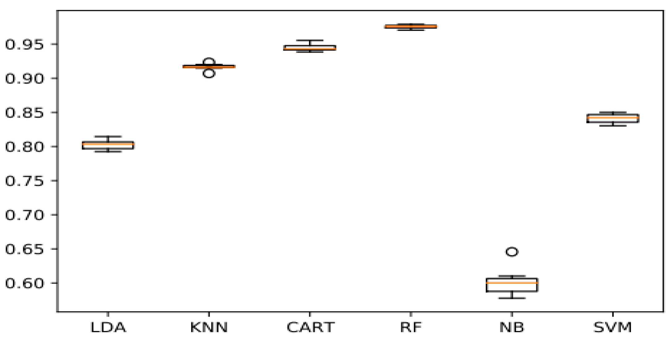
| RF | 97.54% | 97.92% | 97.47% | 97.71% |
| CART | 94.45% | 94.24% | 94.06% | 94.18% |
| KNN | 91.67% | 91.96% | 92.26% | 92.27% |
| SVM | 84.10% | 84.38% | 84.37% | 84.40% |
| LDA | 80.28% | 80.01% | 79.94% | 79.93% |
| NB | 60.09% | 68.65% | 59.95% | 54.74% |
| Activation Function | Accuracy | Precision | Recall | F1-score |
|---|---|---|---|---|
| Adadelta | 80.50% | 81.74% | 81.38% | 81.25% |
| Adagrada | 86.00% | 88.50% | 88.31% | 88.33% |
| Adam | 86.80% | 89.60% | 89.45% | 89.47% |
| RMSprop | 86.30% | 85.75% | 81.78% | 81.03% |
| SGD | 87.60% | 83.86% | 80.06% | 89.41% |
| Activation Function | Accuracy | Precision | Recall | F1-Score |
|---|---|---|---|---|
| Tanh | 89.28% | 91.12% | 91.11 % | 91.08% |
| Sigmoid | 88.95% | 90.94% | 90.86% | 90.88% |
| Softmax | 87.27% | 88.52% | 87.75% | 87.57% |
| Softsign | 89.50% | 91.30% | 91.28% | 91.29% |
| LeakyReLu | 87.06% | 91.00% | 90.95% | 90.96% |
| Swish | 90.10% | 91.35% | 91.88% | 90.77% |
| Elu | 89.25% | 86.57% | 83.48% | 83.31% |
| ReLu | 88.73% | 90.50% | 89.87% | 89.72% |
| Softplus | 89.80% | 91.44% | 91.00% | 90.88% |
| Classifiers | Execution Time (Hour: Min) |
|---|---|
| InceptionV3 (over 100 epochs) | 14 h 20 |
| LDA | 8 h 30 |
| VGG16 (over 100 epochs) | 22 h 35 |
| VGG19 (over 100 epochs) | 29 h 46 |
| ResNet50 (over 100 epochs) | 32 h 21 |
| CNN (over 100 epochs) | 27 h 45 |
| KNN | 7 h 17 |
| CART | 9 h 28 |
| RF | 6 h 55 |
| NB | 4 h 32 |
| SVM | 10 h 35 |
| Optimizers | Advantages | Disadvantages |
|---|---|---|
| SGD | The computation time for each update is not depending on the overall number of training samples, and many computations cost is being saved. | It is challenging to select an appropriate learning rate, as well as using the same learning rate for all the parameters is inadequate. The solution in certain cases might be trapped at the saddle point. |
| Adagrad | At the beginning of training, the accumulative gradient is smaller, the learning rate is higher, and the learning speed becomes faster. It is adequate for addressing sparse gradient problems. | As the training time expands, the cumulative gradient becomes increasingly larger, causing the learning rate to tend toward zero, leading to inefficient parameter updates. |
| Each parameter’s lr is tuned in an adaptive way. | ||
| An efficient optimizer holds information about pseudo curvature and can cope with stochastic objectives very successfully, which makes it relevant and applicable to batch learning. | ||
| RMSProp | RMSProp converges more swiftly than SGD. | The learning rate must be chosen manually. |
| Adadelta | Addressing the inefficient learning problem in the later phase of AdaGrad. It is convenient for the optimization of non-convex and non-stationary problems. | During The late training phase, The updating process might be repeated around The local minimal value. |
| Adam | The gradient descent process is quite steady. It suits mostly non-convex optimization problems with both large datasets and wide dimensional space. | The technique may fail to converge in some instances. |
Disclaimer/Publisher’s Note: The statements, opinions and data contained in all publications are solely those of the individual author(s) and contributor(s) and not of MDPI and/or the editor(s). MDPI and/or the editor(s) disclaim responsibility for any injury to people or property resulting from any ideas, methods, instructions or products referred to in the content. |
© 2023 by the authors. Licensee MDPI, Basel, Switzerland. This article is an open access article distributed under the terms and conditions of the Creative Commons Attribution (CC BY) license (https://creativecommons.org/licenses/by/4.0/).
Share and Cite
Orchi, H.; Sadik, M.; Khaldoun, M.; Sabir, E. Automation of Crop Disease Detection through Conventional Machine Learning and Deep Transfer Learning Approaches. Agriculture 2023, 13, 352. https://doi.org/10.3390/agriculture13020352
Orchi H, Sadik M, Khaldoun M, Sabir E. Automation of Crop Disease Detection through Conventional Machine Learning and Deep Transfer Learning Approaches. Agriculture. 2023; 13(2):352. https://doi.org/10.3390/agriculture13020352
Chicago/Turabian StyleOrchi, Houda, Mohamed Sadik, Mohammed Khaldoun, and Essaid Sabir. 2023. "Automation of Crop Disease Detection through Conventional Machine Learning and Deep Transfer Learning Approaches" Agriculture 13, no. 2: 352. https://doi.org/10.3390/agriculture13020352
APA StyleOrchi, H., Sadik, M., Khaldoun, M., & Sabir, E. (2023). Automation of Crop Disease Detection through Conventional Machine Learning and Deep Transfer Learning Approaches. Agriculture, 13(2), 352. https://doi.org/10.3390/agriculture13020352