Abstract
Conceptualized by the Food and Agriculture Organization in 2010, climate-smart agriculture aims to simultaneously tackle three main objectives. These are increasing food security, building the resilience of agricultural systems for adaptation to climate change and mitigation of GHG. As much research focuses on one of these three objectives, our understanding of how agricultural systems address these three challenges simultaneously is limited by the lack of a comprehensive evaluation tool. In order to fill this gap, we have developed a generic evaluation framework that comprises 19 indicators that we measured in a sample of 12 representative farms of the North Basse-Terre region in Guadeloupe. The evaluation revealed clear differences in the performance of these farming systems. For example, nutritional performance varied from 0 to 13 people fed per hectare, the average potential impact of climatic conditions varied from 27% to 33% and the GHG emissions balance varied from +0.8 tCO2eq·ha−1 to +3.6 tCO2eq·ha−1. The results obtained can guide the design of innovative production systems that better meet the objectives of climate-smart agriculture for the study region. The evaluation framework is intended as a generic tool for a common evaluation basis across regions at a larger scale. Future prospects are its application and validation in different contexts.
1. Introduction
Agriculture strongly affects ecosystems worldwide and is the cause of a broad range of environmental, economic and social issues at the local and global scales [1]. Agriculture, as the second major source of greenhouse gases, greatly contributes to global climate change, which is accelerating and pushing natural Earth systems into a new state [2]. This change has been characterized by a rise in average temperatures, changes in rainfall amounts and distribution, and an increase in extreme climate events, such as hurricanes and droughts [3].
Agriculture is not only contributing to climate change but is also being severely impacted by it. To address this issue, the FAO proposed that agriculture should evolve and adapt to climate change and the mitigation of greenhouse gases (GHG), in addition to sustainable increases in farm productivity, by introducing the concept of climate-smart agriculture [4,5]. Climate-smart agriculture (CSA) is an approach for agricultural systems to support food security under new climatic conditions. In addition to the adaptation and mitigation of climate change and the insurance of food security, the objective of climate-smart agriculture is to increase the adaptive capacity of farmers and resilience and resource use efficiency within agricultural production systems. The intertwining of policies, private investment and landscape affects the implementation of CSA [6,7].
Each farm develops in a particular pedoclimatic, social and economic context; the results of their sustainability assessments can vary with regard to constraints and opportunities in the context. Stakeholders are often seeking context-specific tools and are interested in comparing results with other regional producers, using a tool to take into account the regional context, arguing that the harmonization of assessment tools can be detrimental [8,9]. However, a context-specific approach is less suitable for comparing the performance of different sectors, and countries and may overlook global sustainability issues; this highlights the dilemma between generic and specific approaches [10,11].
Survey- and indicator-based assessment tools are the most widely used for the agricultural sector [8,12]. Although key principles were defined for the selection of indicators, literature reviews show that they vary widely in scoring methods, context-specificity and assumptions [9,13]. This is due to differences in value judgments, prioritizations in the selection of indicators, spatial and temporal scales, system boundaries, and target groups [14]. In addition, in trying to capture overall the sustainability of production systems, an important number of indicators are used for covering each aspect of the sustainability dimensions [15,16,17]. The SAFA guidelines are a typical example where 118 indicators representing 22 themes and 5 dimensions were proposed for defining universal sustainability goals and establishing a widely accepted layout for sustainability in agriculture and food [18]. Therefore, to address the complexity of interpreting such a large number of indicators, normalization and aggregation are common steps after indicator measures are quantified to deduce information and understand losses [19,20].
Comparing farms around the world is nonetheless of great importance as CSA is a global project. Indeed, that could enable the highlighting of regions, territories or nations where CSA is sufficient to determine where solutions can be found to better orient farm design or agricultural policies and landscape planning, or simply to evaluate the performances of a production system compared to others. Generic tools have been developed for sustainability assessments of farms [10,18,21,22], but literature reviews show that no formal and exhaustive method is available for CSA and that there is a need for reliable metrics [23,24]. Some research is underway to develop such tools, but they must rely on an important number of indicators to cover the three pillars of CSA [25].
In the present study, we argue that current CSA assessment tools could be improved with regard to their completeness (targeting the three pillars) and significantly simplified through a holistic approach toward agricultural issues. This development could be interesting when the goal is the comparison of farming systems at the global scale for (1) stakeholder comparisons of local and international performances or (2) the selection of promising farming systems and landscape planning.
CSA targets a sustainable “triple-win” objective [4], and this concept encompasses most present and future agricultural issues. In doing so, CSA is a relevant concept for building a farm-level generic metric assessment framework. The aim of this study was to propose and apply a relevant short, transparent and easy-to-implement set of farm-level indicators for a holistic and generic assessment of CSA. The target group is stakeholders seeking a diagnosis method for farms to highlight critical performance and improve in the face of climate change issues and for policy orientation at the regional scale to facilitate the transition toward CSA.
2. Materials and Methods
2.1. Study Site
The assessment framework was applied in Guadeloupe, a French Overseas Department of the West Indies in the Caribbean (latitude 16°13′ N, longitude 61°34′ W). Guadeloupe is an archipelago (1628 km2) comprising two main islands, Basse-Terre (848 km2) and Grande-Terre (586 km2), with high variations in an ecological context. Sierra et al. [26] divided the archipelago into five agroecological regions that are homogeneous in terms of soil type and climate conditions. This study focused on a specific region, Nord Basse-Terre, of approximately 360 km2 and with 92,000 inhabitants [27]. This agroecological region is characterized by an annual mean temperature and rainfall of 25.4 °C and 2300 mm·year−1, respectively, and kaolinitic ferralsols developed from old volcanic ash deposits.
2.2. Characterization of Farming Systems and Their Diversity
To determine to what extent the study region met the objective of CSA, the diversity of existing farming systems was first characterized with a farm typology. Crop rotations represent the outputs of farmers’ decisions based on their objectives, constraints and biophysical context. To build the farming system typology, data were used on crop acreages, slopes and farm size, which are easily available worldwide based on surveys or databases, such as the IACS for the European Union [28]. In this study, the 2010 governmental farmers’ declaration data of areas and crop rotations of the farming system (methodology described in Todoroff et al. [29]) was used as input data to build up a typology, which represented approximately 80% of the agricultural fields of the archipelago. According to those data, the region comprised 849 farms representing 5035 ha (i.e., 18% of the whole archipelago’s agricultural land area). The typology was obtained following the method detailed in Chopin et al. [30], combined with principal component analysis of the proportion of crops in farm areas with a hierarchical ascending clustering on the resulting principal components to obtain four groups of farms. For each of the four types of farms established from the typology obtained, three farms were randomly selected and surveyed (stratified sampling). To scale up, the assessment results were extrapolated to the whole farming system of the study region using the share (in terms of acreage) of each group.
2.3. Define the Objectives and Boundaries
A list of generic indicators of CSA that could be relevant to most biophysical contexts articulating the key concept of sustainable food security, GHG mitigation and adaptation of agricultural systems was defined. In this study, CSA encompassed economic, social and environmental components of sustainability, reorganizing these three classical dimensions into the three pillars of CSA, placing climate change issues at the center.
The indicators were selected and designed to be relevant, easy to understand, reliable and based on easily accessible data, following the recommendations of Bockstaller et al. [31]. The assessment, carried out at the farm scale, is more relevant for farmers and is readily upscalable for decision-makers and regional policies. Some indicators are related to on-site issues (e.g., “Irrigation/rainfall”, “SOC (soil organic carbon) variation”), while others are related to off-site issues (e.g., “GHG emissions”, “%Renewable”). Energy and material flows are accounted for during a whole crop rotation and until production reaches the farm gate and then converted for one hectare and one year of production. Figure 1 is a representation of the boundaries of the conceptual model of farms used in this research.
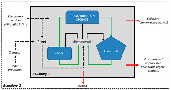
Figure 1.
Boundaries of a conceptual farm. The on-farm boundary 1 (solid black line) was used for 16 out of 19 indicators. The off-farm boundary 2 (dotted black line) was used for 3 holistic indicators, i.e., the energy index of renewable flow and the indicators of potential climate impact and GHG emissions. Dotted and solid black arrows refer to flows before and after on-farm management respectively. Green arrows refer to internal flows and red arrows refer to flows leaving the on-farm boundary 1.
2.4. Construction of the Set of Indicators and Its Calculation
The first step was to define the three CSA pillars and their attributes. The three classical dimensions, economic, social and environmental [32], were taken into account for the definition of these three pillars. During successive workshops and oral presentations between researchers/technicians, farmers and decision-makers, the indicators covering those three dimensions were selected to describe the outcomes with regard to the three pillars of CSA. The selection should respond to the four main characteristics of a good indicator, with a reduction in the number of indicators when (1) the indicators are redundant (one can be estimated from the other) and (2) they are not generic enough for comparison between farms from contrasting contexts. We followed a holistic understanding of the farms in order to obtain as small a set of indicators as possible. To obtain indicators that were as generic as possible, we took into account the regional context when relevant, e.g., for the indicator “Irrigation/rainfall”, we weighted the annual farm water requirements by the annual volume of rainwater intercepted by the farm area. Figure 2 is a synthesis of the indicators of each pillar used in this study and for CSA assessment at the farm scale.
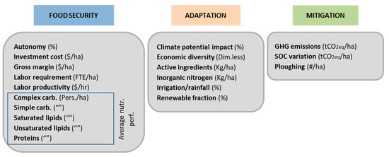
Figure 2.
Synthesis of the indicator framework based on the “Triple-win” objectives of food security, adaptation and mitigation.
2.5. Indicators Selected and Calculation Methods
2.5.1. Food Security
1- Autonomy (%)
The indicator of autonomy measures the farmer’s dependency on public support. Although agricultural subsidies have beneficial effects on employment in some cases [33,34], most studies associated farm dependency with negative outcomes [35,36] and significant issues either on out-farm migration/rural employment [37], environmental impact [38,39] or technical efficiency [40]. These issues are directly related to food security. Thus, it is important to have an overview of farmers’ dependency on public support and then analyze their interactions with sustainability levels during the codesign of farming systems.
Income = gross margin − amortization − fix charges − taxes (US$/year)
Gross margin = gross product − variable cost + subsidies (US$/year)
Gross product = value of commercialized products (US$/year)
2- Investment Cost (US$/ha)
The investment cost measures the amount of investment of equipment and inputs per hectare. This indicator reflects both economic (feasibility) and social (risk) aspects impacting the rate of adoption of the system and, therefore, its potential role in food security improvement. It could be weighted by a regional economic indicator (e.g., gross domestic product, saving per capita) to take into account the economic context, but the value itself is more relevant, and its conversion into USD was considered sufficient to make this indicator generic.
Investment cost: capital invested for the installation and the first year of production, including fixed and variable charges (US$)
Ta: total area of the farm (ha)
3- Gross Margin (US$/ha/year)
This indicator provides important information about economic performance per unit area. In addition to providing information about the acceptability of the system, it addresses the available agricultural land area (ALA) and its potential employment creation rate at the regional scale and, therefore, the potential role of the system in improving food security. As for the investment cost, conversion into USD was considered more relevant and generic than the weighting by another local economic indicator. It takes into account the labor cost; then, the wage of the household labor is subtracted from the gross product.
Gross product = value of commercialized products (US$/year)
Variable costs: labor (including family labor), fuel, fertilizer, etc. (US$/year)
Ta: total area of the farm (ha)
4- Labor Requirement (FTE/ha/year)
Labor requirements were used to evaluate the significance of the farm on employment at the regional scale and then the impact of the adoption of new practices or farming systems. This indicator gives information on the rural employment potential of the system, which is indirectly related to food security. The average standard annual full-time equivalent (FTE: 1650 h in this study) needed to be adapted in relation to the region under study to make the indicator generic.
Labor: total labor (including direct services and family labor) (hr/year)
Ta: total area of the farm (ha)
5- Labor Productivity (US$/h)
This indicator is a measure of the work efficiency of a household. It is based on the gross margin and takes into account labor costs (including family labor) at the hourly minimum rate applied in the study region. It provides information directly on the technical efficiency and attractiveness of the system and indirectly on working conditions, impacting both its potential adoption and role in addressing food security. Improving labor productivity in the agricultural sector is also a way of reducing inequalities at the regional scale [41,42].
Gross margin = gross product − variable cost (inputs, labor, etc.) (US$/year)
Gross product = value of commercialized products (US$/year)
Labor: total labor (including direct services and family labor) (h/year)
6- Complex and Simple Carbohydrates, Saturated and Unsaturated Lipids, and Protein Performances (Pers./ha/year)
These indicators are measures of the ratio between the annual macronutrient production of the farm and the average daily reference intakes. They may be the most important indicator of food security because they are directly related to food production efficiency, which is the first issue to address in a fast-growing world population. Moreover, sustainable or agroecological management can be more context-dependent, making yield gaps an important issue regarding their ability to feed people [43,44]. In this study, we considered an average 2800 kcal·day−1 with 7.5% from saturated lipids, 15% from unsaturated lipids, 10% from simple carbohydrates, 55% from complex carbohydrates and 12.5% from proteins [45,46]. Finally, this indicator addresses the issue related to the reduction in production diversity (linked to malnutrition) that can accompany policies of agricultural intensification [47].
P: edible animal (PA) and vegetal (PV) protein production (g/year)
CA: edible complex (CAC) and simple (CAS) carbohydrate production (g/year)
LI: edible saturated (LIS) and unsaturated (LIU) lipid production (g/year)
INPUT: inputs of edible animal (INPUTPA) and vegetal proteins (INPUTPV), simple (INPUTCAS) and complex (INPUTCAC) carbohydrates, and saturated (INPUTLIS) and unsaturated (INPUTLIU) lipids (g/year)
w: proteins (P), complex (CAC) and simple (CAS) carbohydrates, saturated (LIS) and unsaturated (LIU) lipids, reference intake (g/pers./day)
δ: Assimilation rate for animal (A: 95%) and vegetal (V: 80%) proteins in humans
Ta: Total area of the farm (ha)
We considered the average value of those five indicators as the “average nutritional performance”, which is a tradeoff between quantity and quality and a useful value for interpreting other indicators. The minimum value of these five indicators could be considered, but we should also take into account the complementarity of farm production at the regional scale.
2.5.2. Adaptation
1- Climate Potential Impact (%)
Vulnerability to climate change is a function of Sensibility * Exposure * Adaptive capacity [48]; however, adaptive capacity was not taken into account in the indicator “climate potential impact” proposed here for two main reasons: (1) it is complex because it depends on many variables, mainly social, technological and economic, from the field to the national scale [49,50], that should be specifically studied in relation to stakeholders, such as industrials, insurers, politicians, associations, the media, schools, communities and consumers; (2) at the farm scale, adaptive capacity is also closely related to the overall performance of the indicator framework proposed here. For example, level of autonomy is an indicator of the capacity of a farmer at the local level to make rapid decisions with regard to the farm’s surrounding environment or for labor productivity, which brings indirect information about the potential asset of a household. Finally, the economic diversity indicator (see below) also provides information about the resilience of the system, which is related to adaptive capacity. For these reasons, the factor “Adaptive capacity” was not taken into account, and the indicator was a function of Sensibility * Exposure.
We evaluated those two variables with a “semiquantitative” approach on a High (3)—Medium (2)—Low (1)—Negligible (0) scale for the five following hazards: flooding, drought, temperature rise, sea level rise and cyclones [51]. The scale followed an index-based methodology relying on (1) 6 “agroclimatic indicators” for the assessment of field exposure to climate hazards and (2) 22 indicators for the assessment of field sensitivity, split into three dimensions: “crops biology and ecophysiology”, “landscape characteristics” and “agricultural practices”. In this study, (biophysical) exposure was strictly the magnitude, intensity or variability of external climate parameters, while (biophysical) sensitivity was strictly the degree to which the biophysical part of the system was (potentially) affected (adversely or beneficially) by climate-related stimuli.
2- Economic Diversity (Dimensionless)
The economic diversity indicator measures the diversity of activities at the farm level, assuming that the greater the number of activities, the higher the economic risk. Agricultural biodiversity is an important lever to improve resilience and climate change adaptation in addition to food security [52,53]. The indicator proposed here is adapted from the “Shannon diversity index” and provides a measure of crop diversity in relation to economic value, i.e., gross margins. We could have shared gross margins between valuable crops (converting self-consumed production into economic values) and crops that cannot be directly valued, but we found it more relevant and generic to take into account only valuable crops for the calculation method. In the case of pastures, we shared the value of livestock production between the different crop species comprising the pasture, with an arbitrary relative abundance above 10% in terms of area (visual estimations). This threshold of 10% could be changed in situations of very high species richness, with similar relative abundances.
GMi: the annual gross margin derived from crop species i (US$/year)
GMT: the total annual gross product (US$/year)
3- Active Ingredients (kg/ha/year)
This indicator is the unique value dealing with ecotoxicological (also the indicator “inorganic nitrogen” to a lesser extent), human health and work conditions pressure, providing a global measure of the amount of pesticide active ingredients used per unit area. It does not take into account the specific toxicity of products or their method of application like other indicators [54] and seems to be one of the less predictive for ecotoxicological impacts [55], but it is easier to use and easily understandable by stakeholders. Moreover, considered here, sharing information about the toxicity effects of different products for the same purpose should be a specific policy task that allows for optimal choices by farmers.
Ai: annual active ingredient input from pesticide i (kg/year)
Ta: total area of the farm (ha)
4- Inorganic Nitrogen (kg/ha/year)
The input of inorganic nitrogen is a proxy indicator for leaching risks when compared with production outputs (food, energy) but also for the dependency of the farms on fertilizers and fossil fuels. In this framework, for the same productivity, the less the system depended on external inputs, the more it relied on ecosystem services and, therefore, the more it was integrated/adapted to its environment. Organic nitrogen was not taken into account for three main reasons: (1) the application rate by farmers can vary greatly from year to year due to socioeconomic constraints, weather hazards or compost quality; (2) organic nitrogen presents a wide range of environmental impacts depending on the age and quality of the amendments, management and yields; and, (3) globally, fertilization with organic materials is a means of recycling terrestrially available N, thereby reducing inputs to the biosphere. Moreover, in 2010, inorganic nitrogen corresponded to more than 51% of nitrogen input in agriculture and approximately 14% of GHG agricultural emissions, while compost/manure applied to soils corresponded to approximately 15% of nitrogen input and 4% of GHG agricultural emissions [56,57,58]. Hence, in the actual context of climate change and the increasing scarcity of fossil fuel resources, inorganic nitrogen appears to be a relevant and easier-to-implement indicator of adaptation.
N: total inorganic nitrogen input (kg/year)
Ta: total area of the farm (ha)
5- Irrigation/Rainfall (%)
This indicator provides important information about the dependency and pressure of the farm on water resources and its level of integration/adaptation in the agroecological region under study.
Rr: rainfall of the study region (m/year)
Ta: total area of the farm (m2)
Irrigation water: volume of water from the irrigation grid (m3/year)
6- Renewable Fraction (%)
This indicator is inherited from the emergy accounting method, which is one of the most holistic methods for the assessment of direct and indirect energy flows supporting a production system. “Solar emergy is the available solar energy used up directly or indirectly to make a service or product. Its unit is the solar emjoule (abbreviated sej)” [59]. The unit emergy value (UEV) is the amount of embodied energy (expressed in sej) required or used up for one joule of product or service created.
Emergy accounting is a biophysical analysis based on a unique approach considering sunlight, earth-moon-sun gravitational attraction (EMSGA) and earth internal heat (EIH) as the three primary energy sources of all other energies and materials in the biosphere embodied in transformation processes. The EMSGA and EIH were expressed in relation to solar energy, leading to the two first UEVs, renamed the SER (solar equivalence ratio) because, strictly speaking, the EMSGA and EIH are not produced from solar energy. However, in doing so, the emergy method provides one universal energy unit: the “solar emergy joule” (sej); three initial energy sources: sunlight, EMSGA and EIH; and three initial SER: 1 sej/J of sunlight, 30,900 sej/J of EMSGA and 4900 sej/J of EIH.
From this starting point, this method enables the UEV calculation of ecosystem services to anthropogenic goods and services by tracing back all energy flows on the same unit basis. A significant body of literature on the emergy assessment framework is available [60].
After defining the boundary of the system, different indicators can be calculated from emergy accounting. One of them is the “renewable fraction” as the renewability of energy is an important factor in adaptation and mitigation strategies [61]. The indicator “renewable fraction” was calculated following the methodology of Odum [59] and also accounting for the renewable fraction of purchased inputs as proposed by Cavalett et al. [62]:
Y: the total emergy released (sej/year)
Emi: the emergy content of input i (sej/year)
%Renewablei: the renewable fraction of input i (%)
2.5.3. Mitigation
1- Greenhouse Gas Emissions “GHG Emissions” (tCO2eq/ha/year)
The GHG Protocol Corporate Standard classifies GHG emissions into three “scopes” [63]. Scope 1 emissions are direct emissions from owned or controlled sources; scope 2 emissions are indirect emissions from the generation of purchased energy and scope 3 emissions are all indirect emissions (not included in scope 2) that occur in the value chain of the system. Moreover, for various categories of emissions activities, the IPCC guidelines [64] provide several options for calculating emissions, described as “tiers”. There are three levels of tiers: tier 1, tier 2 and tier 3, referring to calculation method accuracy. In the present framework, measuring GHG emissions was proposed using the “tier 1” method and “tier 2” to a lesser extent when data are available. The tier 1 frameworks are less accurate than others but “are designed to use readily available national or international statistics in combination with the provided default emission factors and additional parameters provided, and therefore should be feasible for all countries” [64]. The use of such an indicator would ease the comparison of many farming systems. Removal of GHG through CO2 sequestration is not included in the “GHG emissions” indicator but in the “SOC variation” indicator, accounting for soil organic carbon stock variation (see below). Figure 3 presents an illustrative diagram of the different gas flows taken into account. This indicator is meaningful when comparing it with nutritional performance, giving a value expressed in terms of “fed person·tCO2eq−1”. In this way, we combine two elements of mitigation and food security dimensions.
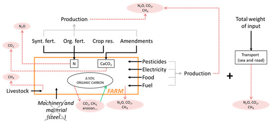
Figure 3.
Description of the gas flows that were taken into account for estimating greenhouse gas emissions (“GHG emissions”) of the farm represented with the orange line. Black, green and red dotted arrows refer to inputs, gas emissions and CO2 sequestration respectively. Synt. Fert., Org. fert. and Crop res. refer to Organic fertilizers, Synthetic fertilizers and Crop residues respectively. The variation (∆) of soil organic carbon was accounted for separately with the indicator “SOC variation”. Emissions related to machinery and other materials (crossed out in gray) were not taken into account.
2- Soil Organic Carbon Variation “SOC Variation” (tCO2eq/ha/year)
Soil organic carbon (SOC) stock variation is an indicator that provides information about soil resilience. For the same productivity, improving SOC stock is also related to sustainable agricultural practices such as compost amendment, reduced tillage, erosion control, perennial crops, etc., or will be improved through these practices. This is another example of a holistic understanding of farms in order to reduce the set of indicators. Moreover, carbon sequestration in soils is an important strategy of GES mitigation, spotlighted as part of the “4/1000 initiative” project [65,66].
This indicator is more complex to calculate as it requires data on soil initial C content, the input of biomass as residues or organic fertilizers, the mineralization of inputs, potential erosion and biomass humification. When experimental data are missing, those variables should be estimated from the literature. For the purpose of this study, this indicator was calculated with the Morgwanik model described by Sierra et al. [26]. We applied this indicator to each farm’s cropping system for a whole crop rotation over a 30-year period. In this study, the current (initial) SOC stock (C0) was determined according to the Soil Database of the Agricultural Engineering Office (SDAEO) CaribAgro in Guadeloupe [26]. To convert the soil carbon variation into CO2eq, we approximated that CO2 was the only gas emitted from agricultural soils [67]. In doing so, both “GHG emissions” and “SOC variation” could be subtracted to estimate the GHG balance.
Cn: soil organic carbon for the year n (t/ha)
C0: soil organic carbon for the year 0 (t/ha)
km: soil mineralization rate (%)
Ke: soil erosion rate (%)
Kh: amendment humification ratio (%)
Kh’: crop residues humification ratio (%)
Am: carbon inputs from amendment (t/ha)
Res: carbon inputs from crop residues (t/ha)
3- Plowing (number/year)
The indicator proposed here addresses the frequency of plowing. Plowing affects the macrofauna community [68,69], soil structure and fertility [70]. The depth of plowing, machinery load and other machinery traffic were not considered; in this way, the data requirement was reduced while maintaining one of the most important factors of soil health.
PLi: Number of plowings per year in field i
Ai: Area of the field i (ha)
2.6. Data Sources
Data quality and availability are important factors orienting indicator construction or selection. The survey of the 12 farmers provided data on material and energy flows. When data were missing, e.g., the farmer was not able to provide information about a specific yield or input, they were substituted for data from local “gray” literature and, as a last resort, peer-reviewed literature. For each farm, the current (initial) SOC stock was determined according to the Soil Database of the Agricultural Engineering Office (SDAEO) CaribAgro in Guadeloupe [26]. The ADEME and IPCC reports [64,71] provided the data for GHG emissions factors used in tier 1 and tier 2 approaches. Emergy assessment publications provided recommendations for the accounting methodology and specific UEVs used in this study [59,60]. The emergy assessment was carried out using the new geobiosphere emergy baseline of 12.0 × 1024 sej/year [72].
3. Results and Discussion
Four different farm types were distinguished, namely, specialized sugarcane producers (SSP), livestock producers (LP), diversified producers for local and export markets (DPLE) and diversified producers for local markets (DPL), representing 560 (2745 ha), 183 (906 ha), 72 (1287 ha) and 34 (97 ha) farms, respectively. The farming system was mainly characterized by sugarcane and pastoral activities (Figure 4). In this farming system, sugarcane and banana are mainly cultivated to be exported to mainland France. Sugarcane and its straw can also be used as fodder for livestock. Other productions are dedicated to the local market. SSPs mainly grow sugarcane on farms with an average area of 4.9 ha and very limited area of spare land. LPs have approximately two-thirds of their land for pasture where livestock extensively grazes and one-third for sugarcane. DPLE has a diversified cropping plan with sugarcane for approximately one-third and pineapple, plantain and tuber production, including mainly yam. Finally, DPLs mainly produce fruits from orchards and vegetables in market gardening cropping systems. Sugarcane and pasture are also represented in a minor proportion of the area, accounting for 9%.
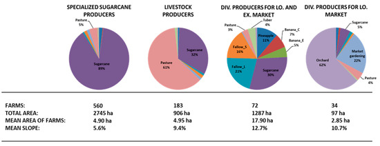
Figure 4.
Typology of the farming system located in the region of North Basse-Terre based on crop rotation data from the governmental declaration database AGRIGUA of 2010. The four clusters were obtained through a hierarchical ascending classification using the principal components of interest (Kaiser criteria) from a principal component analysis. Each color corresponds to a different activity, the main ones are specified in the chart. Banana_C, Banana_E, Fallow_S, Fallow_L, correspond to banana of local varieties, Cavendish banana for export market, short fallows and long fallows (> 8 months) respectively.
Table 1 presents the average values of the 19 indicators for the three farms from each farm type. The last column is the simple extrapolation of the scores to the entire study region based on the typology. Figure 5 presents the radar charts highlighting the relative performances of each farm type for food security, adaptation and mitigation.

Table 1.
Results of the climate-smart assessment framework. The 19 indicators for each farm type (“specialized sugarcane producers” (SSP), “livestock producers” (LP), “diversified producers for local and export markets” (DPLE) and “diversified producers for local markets” (DPL)) were calculated as the average value of the three farms surveyed. The last column, “weighted mean”, was based on the area represented by each farm type and corresponds to the performance of the farming system.
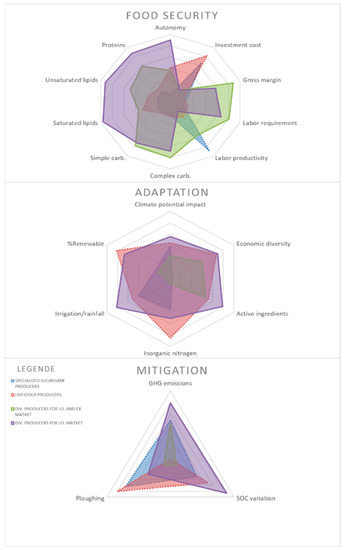
Figure 5.
Radar charts of the relative scores for each dimension (food security, adaptation and mitigation). After mean-centering the scores, we multiplied by -1 the values of indicators that should decrease (Investment cost, Active ingredients, Inorganic nitrogen, Irrigation/rainfall, Potential climate impact, Plowing, GHG emissions) in order to obtain the same reading. Higher values corresponded to better performances.
3.1. Food Security Outcomes
The farming systems under study had on average autonomy of −20% with regard to subsidies. According to the calculation method, this value indicates that the average farmer’s income without subsidies was negative and represented −20% of the total income. In comparison, the average autonomy of farms in the European Union was +64% from 2014 to 2018 [73]. This result highlighted the low profitability and high dependency with regard to policy orientation toward farms from each category, especially for the SSP (−42%), which was widely represented in the study region. The DPL, characterized by orchards and market gardening activities, presented higher autonomy (+57%) but represented only 97 ha of the ALA (Figure 4, Table 1).
The average investment cost and gross margin of the farming systems were 8600 US$/ha and 3300 US$/ha, respectively. Both the DPLE and the DPL had higher gross margins of 5500 US$/ha and 4200 US$/ha, respectively. They also presented higher investment costs but with higher autonomies and higher contributions to employment, with 0.3 and 0.2 full-time equivalent (FTE) per hectare.
With an average of 0.1 FTE per hectare, the regional farming systems only represented 450 direct jobs for an estimated 91,000 inhabitants in the study region [27]. In terms of labor productivity, the average value was US$ 23/h, but the SSP paid US$ 32/h, approximately twice as high as the values for the LP and DPL groups. This high labor productivity was due to a combination of very low labor requirements with high governmental subsidies allocated to sugarcane crops.
At the regional level, the average nutritional performance was 3 pers./ha, corresponding to approximately 13,500 “well-balanced” nourished persons or 15% of the population. However, this indicator widely ranged from approximately 0 pers./ha for the SSP and LP to 13 pers./ha for the other farm types. The very low nutritional performances of the SSP and LP were due to the overrepresentation of sugarcane monoculture (sugarcane was not considered as human food in this study except through meat production) and the extensive management of livestock. Indeed, farmers in the study region are frequently in part-time farming situations and first use livestock as a saving strategy and for landscape management. Globally, the results of nutritional performance were mainly supported by simple carbohydrate production, while complex carbohydrate, protein and lipid production are important limiting factors (Table 1). Through this indicator, we attempted to improve the “crop diversity” indicator used in the RHoMIS tools [22] by taking into account the nutrient value of crops, which can largely vary among different species or be very similar. We also used these nutritional performances as a measure of productivity instead of energy (kilo-calories), as found in other CSA assessments [22,74], as crop nutrient content data are easily available.
The radar chart (Figure 5) shows that the DPL globally better satisfied the food security dimension. However, their lower labor productivity and higher investment cost could be important factors explaining the low representation of this farm type in the ALA.
3.2. Adaptation Outcomes
The estimated current climate potential impact through the five hazards, i.e., drought, flooding, temperature rise, sea level rise and cyclones, on the farming systems was 28%. According to the calculation method, these values indicate that the current climate hazard reached 28% of the theoretical maximum impact from which current cropping systems can recover. This value is useful to compare the effects of new activities or agricultural practices’ adoption with regard to the climate context. At the farm-type level, the results show lower potential impacts for both the DPL (27%) and the LP (28%) (Table 1).
The average value of economic diversity based on the Shannon index was 0.8, measuring the heterogeneity (also associated with “disorder and uncertainty”) of the gross margins associated with different crop species. Higher values indicated higher heterogeneity and thus higher diversity. To our knowledge, substituting species for gross margins in the Shannon index is not found in the literature. It is proposed here as a way of overcoming the methodological issue of comparing the abundance of different crop species. As a new indicator, its value cannot be compared to other studies at this time, but it can be used to compare different production systems. This indicator shows important differences, with much higher values for both the DPL (1.5) and the LV (1.5) than for the DPLE (1.1) and SSP (0.3), indicating a higher diversity of gross margins origin and thus lower potential impacts in the case of economic, social or climate perturbations.
In terms of agricultural inputs, an average of 4.4 kg/ha of pesticide active ingredients and 70 kg/ha of inorganic nitrogen were used at the regional level. In comparison, an average of 2.9 kg/ha of active ingredients and 155 kg/ha of inorganic nitrogen are used at the national level [75,76,77]. At the farm type level, pesticide inputs for the LP (2.6 kg/ha) and DPLE (2.7 kg/ha) showed similar results. The DPL and SSP had lower and higher values of 1.7 kg/ha and 4.7 kg/ha, respectively. With regard to the average nutritional performances obtained in the present study, the regional farming systems used an average of 23 kg/ha of inorganic nitrogen per nourished person. However, the DPL presented higher performances, with approximately 4 kg/ha of inorganic nitrogen per nourished person.
Globally, water used corresponded to 6% of the average volume of rainwater falling on farms. However, the DPLE presented a value of 11%, showing a stronger reliance on irrigation water and thus a stronger impact on water resources compared to other farm systems. This indicator also provides information about the level of adaptation based on integrated practices with regard to the climate context (i.e., crop species, crop rotations, etc.). For example, the development of agroforestry or the selection of species and varieties that are better adapted to the agroecological region can reduce the value of this indicator.
The production processes of the farming systems relied on 25% renewable energy, with values ranging from 22% for the DPLE to 35% for the LP. In comparison, the agricultural production of Italy relied on 28% of renewable energy [78]. More recently, Zhang et al. [79] calculated the renewable fraction of two traditional and two modern types of farms in China and showed that values ranged from 27% to 65%. In Iran, greenhouse tomato production systems were analyzed and showed that the renewable fraction of the production process ranged from 14 to 19% [80]. This holistic indicator is very important as it accounts for all renewable ecosystems and anthropogenic flows in the production system and is closely related to sustainability; its improvement should be a major task in CSA development.
The radar chart shows that, globally, both the DPL and the LP had a better satisfaction with the adaptation pillar (Figure 5). These results seem to highlight a correlation between the autonomy of the farms and their global adaptation performances.
3.3. Mitigation Outcomes
The average regional value of GHG emissions was 1.9 tCO2eq/ha, ranging from 1.0 to 3.4 tCO2eq/ha for the DPL and LP, respectively (Table 1). In comparison, the GHG emissions of farms at the national level reached 3.2 tCO2eq/ha in 2015 [81].
The average SOC variation was −0.5 tCO2eq/ha, ranging from -0.8 tCO2eq/ha to +0.2 tCO2eq/ha for the DPLE and DPL, respectively. Subtracting the SOC variation value from the GHG emissions gave a GHG balance of +2.4 tCO2eq/ha (Table 1). This value could be weighted with nutritional performance. At the regional scale, the farming systems emitted, on average, 0.8 tCO2eq per nourished person, but this value ranged from 0.1 tCO2eq to 12.3 tCO2eq emitted per nourished person for the DPL and SSP, respectively. Applying the national objective of GHG reduction by a factor of 4 before 2050 [82] to the agricultural sector and considering the −17% reduction already achieved since 1990 [83], a remaining 70% reduction must be achieved before 2050. This reduction would bring the average GHG balance from the current 2.4 tCO2eq/ha to 0.7 tCO2eq/ha. SOC sequestration has limited potential in quantity and will reach a physical limit in time in the best scenarios [84], and these points were presented in part as justification for not including this parameter in CSA assessments [74]; however, at this time, it (1) remains a significant lever in mitigation policies [66], (2) may instead decrease if inappropriate practices are adopted, and (3) is an important proxy for sustainable agricultural practices (e.g., compost amendment, erosion management, reduced tillage, biomass reuse, etc.) in a ”triple-win” approach.
Numerous agroecological practices provide efficient solutions for improving mitigation, such as agroforestry systems in which large amounts of carbon can be sequestered through perennial biomass [85,86]. As agroforestry practices were marginal in terms of acreage in the farms studied, perennial biomasses were not accounted for but should otherwise be included in the GHG balance.
The plowing intensity is one of the important factors of SOC variation and ranged from 0.3 to 1.6 plowing/ha for the LP and DPLE, respectively, with an average value of 0.8 plowing/ha at the regional scale. These results indicate a low pressure of farmers’ practices related to soil plowing but also highlighted the risk of increasing SOC losses with the adoption of new agricultural activities requiring more soil preparation than sugarcane crops or pasture. Nevertheless, factors such as the depth of plowing or the weight of machinery were not taken into account in this indicator. Overall performance of the farming systems for the mitigation pillar was better satisfied for the DPL and, to a lesser extent, the LP (Figure 5).
3.4. Summary of Results and Limits of the Method
The set of indicators distinguished different levels of sustainability through the three pillars of CSA and highlighted the diversity of farms of a small pedoclimatic region (Table 1, Figure 5). Overall, the financial autonomy of farmers was low, but some can serve as a model, i.e., the DPL type, which also corresponds to the smallest farms. This financial autonomy and the gross margin are important points with regard to farm resilience [87] but were also linked to higher investment costs and lower labor productivity in this context. Sugarcane monoculture and extensive livestock management led to very low nutritional performances for the SSP and LP types compared to other types. Nutrient production is far from satisfying regional food needs and is clearly unbalanced in favor of simple carbohydrates, despite sugarcane not being considered a food crop. Through the adaptation pillar, the DPL and LP types showed better performances for all indicators. They presented higher resilience through lower potential climate impacts, higher economic diversities and more renewable energy flows. Both the DPL and LP types also presented lower environmental impacts with reduced use of pesticides and inorganic nitrogen and less pressure on water resources.
Finally, in terms of mitigation potential, the DPL type also presented better performances in terms of GHG emissions and SOC variation, notwithstanding the plowing intensity, which was the second most intensive. However, the four types remained GHG-emitting agricultural systems, and management adaptation must continue to be explored in order to reach net zero CO2 emissions by 2050 and limit warming to 1.5 °C [88], as per the Paris Agreement.
As synthesized in Figure 2, the food security pillar was characterized as a combination of farmers’ financial autonomy, productivity, nutritional balance and economic performance. The adaptation pillar was characterized as a combination of farms’ integration into their pedoclimatic environment, environmental impacts, the durability of production, economic diversity, renewable energy in production flows and potential climate impact. The mitigation pillar was characterized by GHG emissions, carbon sequestration and soil management. The set of indicators attempted to address some gaps in existing assessment methods by clearly taking into account the three pillars of CSA with a multi-dimensional approach to production and including social and economic aspects of sustainability, which have previously been largely ignored [24]. It also attempted to address the spatially variable impact of CSA adoption through the indicator “potential climate impact”, which takes into account pedoclimatic contexts where agricultural practices are adopted. This indicator was specifically described in Selbonne et al. [51].
This set of indicators is not intended to be used for on-farm monitoring because it does not focus on specific agricultural practices or principles but rather aims to provide a large amount of indirect information related to CSA performances. For example, the indicator “economic diversity” of the adaptation pillar provides information about biological diversity and potential ecological and economic resilience; the indicator “SOC variation” provides information about atmospheric CO2 mitigation potential and soil management sustainability; both “inorganic nitrogen” and “nutritional performance” are a proxy for resource use efficiency.
Some shortcomings are apparent in the proposed methodology, the first of which is related to the fact that only researchers participated in the selection of the indicators; the involvement of stakeholders such as farmers may allow for a better consideration of objectives and constraints and better flexibility and applicability [89,90]. Therefore, as mentioned above, we specifically recommend this framework for the ex-post assessment of agricultural policies and interaction between researchers and decision-makers. It can also be used in ex-ante assessments of different agricultural policies through bioeconomic models [91].
Another limitation of the framework was the fact that no indicator or combination of indicators provided information about gender parity. Even if we considered this point as related to upstream issues (cultural, land access), it could be added if it appears as central in a majority of contexts. Moreover, the study was applied to a limited number of farms and, therefore, requires a larger-scale evaluation to verify its genericity and its capacity to respond to other value judgments and conceptions of CSA. The limited number of farms surveyed also impacted the quality of the extrapolation. This shortcoming was partly taken into account by (1) defining a homogenous and small pedoclimatic region and (2) carrying out a stratified sampling according to a typology of farms but could be avoided through larger sampling. Finally, although this framework remains easier to implement than other indicator-based assessment tools with a finer breakdown of the concept of sustainability, as, for example, in the SAFA tool [18], some indicators such as the emergy indicator of “renewable fraction” and the indicator of “potential climate impact” require much data and are more complex to implement. This point should be discussed with stakeholders and more researchers. We believe that the set of indicators we proposed in this study must be tested in diverse contexts to scientifically assess whether it is relevant and generic enough for diverse, real-world situations.
4. Conclusions
This study describes an indicator-based assessment framework (Figure 2) aimed at assessing farm performance with regard to the three pillars of climate-smart agriculture (CSA). A trade-off between comprehensiveness, completeness and genericity was proposed in this study. This approach aims at fostering greater collaboration between stakeholders through the development and assessment of CSA based on common references. CSA was not defined through specific thresholds but as the level of one’s performance with regard to other production systems. The selected indicators were expected to cover all aspects of sustainable CSA by themselves or in combination, directly or indirectly from a holistic understanding of the farming system. Some indicators are meaningful by themselves and others are useful in comparative studies of different systems/scenarios.
In this case study, the main findings are as follows. First, the lowest economic autonomy was associated with the dominant farm types, implying that small changes in support policies would necessarily affect regional farming system performances. Second, the farm types with lower nutritional performance, adaptation and mitigation potential seemed to be favored with the lowest investment costs and higher labor productivity. Third, there is a low nutritional performance of the regional farming system with regard to the population, specifically in terms of protein and lipid production. Significant improvements in the three pillars of CSA could be achieved based on the least represented production systems, i.e., the DPL, which also corresponds to the smallest and most diversified farms. The development of this type of farm must be encouraged. Finally, if specific goals of CSA are targeted, such as carbon neutrality, food sovereignty or no-use of pesticides, designs for innovative production systems could be considered.
The framework succeeded in highlighting differences, strengths and weaknesses between farms of a small agroecological region and appears to be adequate for comparing systems at a larger scale. These results and this framework are currently used for the design of new climate-smart activities and the assessment of different policies and adoption scenarios. The present study described the first two steps of a larger study aimed at developing climate-smart agriculture. To this end, the proposed approach is used for the “prototyping” of new farming systems, following the method of Vereijken [92]. This method represents a good way to cope with the urgency of global changes by (1) providing data on current and innovative farms and (2) creating emulation and knowledge diffusion among stakeholders and encouraging debate on agricultural policies regarding the design and assessment of regional scenarios of transition.
Author Contributions
Conceptualization, S.S. and J.-M.B.; methodology, S.S. and J.-M.B.; software, S.S., L.G.; validation, S.S., J.-M.B., J.S., P.C. and R.T.; formal analysis, S.S., F.C. and L.G.; investigation, S.S., R.T. and F.C.; resources, S.S., J.-M.B., R.T.; data curation, F.C. and S.S.; writing—original draft preparation, S.S.; writing—review and editing, S.S., J.-M.B. and P.C.; visualization, S.S. and J.-M.B.; supervision, J.-M.B., J.S.; project administration, J.-M.B.; funding acquisition, J.-M.B. All authors have read and agreed to the published version of the manuscript.
Funding
This research was funded by ADEME through the Call for Research Proposals GRAINES (project EXPLORER, grant number 1703C0009) and the European Regional Development Fund (FEDER, Guadeloupe Region) projects EXPLORER (grant number 2018-FED-1073), RIVAGE (grant numbers CR/16-1114 and 2015-FED-196) and CAVALBIO (grant number 2015-FED-198).
Data Availability Statement
Data on surveyed farmers are subject to restriction. For more information, please contact the data manager of the National Research Institute for Agriculture, Food and the Environment (INRAE).
Acknowledgments
We would like to thank all the contributors to this study and in particular the 12 farmers who participated in the survey and the two anonymous reviewers and editor for their helpful and relevant comments.
Conflicts of Interest
The authors declare that they have no known competing financial interests or personal relationships that could have appeared to influence the work reported in this paper.
References
- Ecosystems and Human Well-Being: Synthesis; Millennium Ecosystem Assessment (MEA); Island Press: Washington, DC, USA, 2005; ISBN 978-1-59726-040-4.
- Rockström, J.; Steffen, W.; Noone, K.; Persson, Å.; Chapin, F.S.; Lambin, E.F.; Lenton, T.M.; Scheffer, M.; Folke, C.; Schellnhuber, H.J.; et al. A safe operating space for humanity. Nature 2009, 461, 472–475. [Google Scholar] [CrossRef] [PubMed]
- Pörtner, H.-O.; Roberts, D.; Tignor, M.; Poloczanska, E.S.; Mintenbeck, K.; Alegría, A.; Craig, M.; Langsdorf, S.; Löschke, S.; Möller, V.; et al. Climate Change 2022: Impacts, Adaptation and Vulnerability Working Group II Contribution to the Sixth Assessment Report of the Intergovernmental Panel on Climate Change; Cambridge University Press: Cambridge, UK; New York, NY, USA, 2022; 3056p. [Google Scholar] [CrossRef]
- FAO. “Climate-Smart” Agriculture. Policies, Practices and Financing for Food Security, Adaptation and Mitigation; Food and Agriculture Organization of the United Nations: Rome, Italy, 2010; p. 49. [Google Scholar]
- Lipper, L.; Zilberman, D. A Short History of the Evolution of the Climate Smart Agriculture Approach and Its Links to Climate Change and Sustainable Agriculture Debates. In Climate Smart Agriculture; Lipper, L., McCarthy, N., Zilberman, D., Asfaw, S., Branca, G., Eds.; Natural Resource Management and Policy; Springer International Publishing: Cham, Germany, 2018; Volume 52, pp. 13–30. ISBN 978-3-319-61193-8. [Google Scholar]
- Karlsson, L.; Naess, L.O.; Nightingale, A.; Thompson, J. ‘Triple wins’ or ‘triple faults’? Analysing the equity implications of policy discourses on climate-smart agriculture (CSA). J. Peasant Stud. 2018, 45, 150–174. [Google Scholar] [CrossRef]
- Newell, P.; Taylor, O. Contested landscapes: The global political economy of climate-smart agriculture. J. Peasant Stud. 2018, 45, 108–129. [Google Scholar] [CrossRef]
- Gasparatos, A.; El-Haram, M.; Horner, M. A critical review of reductionist approaches for assessing the progress towards sustainability. Environ. Impact Assess. Rev. 2008, 28, 286–311. [Google Scholar] [CrossRef]
- Schader, C.; Grenz, J.; Meier, M.S.; Stolze, M. Scope and precision of sustainability assessment approaches to food systems. Ecol. Soc. 2014, 19, art42. [Google Scholar] [CrossRef]
- Binder, C.R.; Feola, G.; Steinberger, J.K. Considering the normative, systemic and procedural dimensions in indicator-based sustainability assessments in agriculture. Environ. Impact Assess. Rev. 2010, 30, 71–81. [Google Scholar] [CrossRef]
- de Olde, E.M.; Oudshoorn, F.W.; Sørensen, C.A.G.; Bokkers, E.A.M.; de Boer, I.J.M. Assessing sustainability at farm-level: Lessons learned from a comparison of tools in practice. Ecol. Indic. 2016, 66, 391–404. [Google Scholar] [CrossRef]
- Chopin, P.; Mubaya, C.P.; Descheemaeker, K.; Öborn, I.; Bergkvist, G. Avenues for improving farming sustainability assessment with upgraded tools, sustainability framing and indicators. A review. Agron. Sustain. Dev. 2021, 41, 19. [Google Scholar] [CrossRef]
- Velten, S.; Leventon, J.; Jager, N.; Newig, J. What Is Sustainable Agriculture? A Systematic Review. Sustainability 2015, 7, 7833–7865. [Google Scholar] [CrossRef]
- de Olde, E.M.; Bokkers, E.A.M.; de Boer, I.J.M. The Choice of the Sustainability Assessment Tool Matters: Differences in Thematic Scope and Assessment Results. Ecol. Econ. 2017, 136, 77–85. [Google Scholar] [CrossRef]
- Gaviglio, A.; Bertocchi, M.; Demartini, E. A Tool for the Sustainability Assessment of Farms: Selection, Adaptation and Use of Indicators for an Italian Case Study. Resources 2017, 6, 60. [Google Scholar] [CrossRef]
- Zahm, F.; Viaux, P.; Vilain, L.; Girardin, P.; Mouchet, C. Assessing farm sustainability with the IDEA method—from the concept of agriculture sustainability to case studies on farms. Sustain. Dev. 2008, 16, 271–281. [Google Scholar] [CrossRef]
- Talukder, B.; Blay-Palmer, A.; vanLoon, G.W.; Hipel, K.W. Towards complexity of agricultural sustainability assessment: Main issues and concerns. Environ. Sustain. Indic. 2020, 6, 100038. [Google Scholar] [CrossRef]
- Scialabba, N.; Grenz, J.; Henderson, E.; Nemes, N.; Sligh, M.; Stansfield, J.; Lee, S.; Brugère, C.; Bentacur, M.; Kneeland, D.; et al. Sustainability Assessment of Food and Agriculture systems (SAFA) Indicators; FAO: Rome, Italy, 2013. [Google Scholar]
- Pollesch, N.L.; Dale, V.H. Normalization in sustainability assessment: Methods and implications. Ecol. Econ. 2016, 130, 195–208. [Google Scholar] [CrossRef]
- Zhou, P.; Fan, L.-W.; Zhou, D.-Q. Data aggregation in constructing composite indicators: A perspective of information loss. Expert Syst. Appl. Int. J. 2010, 37, 360–365. [Google Scholar] [CrossRef]
- Schader, C.; Baumgart, L.; Landert, J.; Muller, A.; Ssebunya, B.; Blockeel, J.; Weisshaidinger, R.; Petrasek, R.; Mészáros, D.; Padel, S.; et al. Using the Sustainability Monitoring and Assessment Routine (SMART) for the Systematic Analysis of Trade-Offs and Synergies between Sustainability Dimensions and Themes at Farm Level. Sustainability 2016, 8, 274. [Google Scholar] [CrossRef]
- Hammond, J.; Fraval, S.; van Etten, J.; Suchini, J.G.; Mercado, L.; Pagella, T.; Frelat, R.; Lannerstad, M.; Douxchamps, S.; Teufel, N.; et al. The Rural Household Multi-Indicator Survey (RHoMIS) for rapid characterisation of households to inform climate smart agriculture interventions: Description and applications in East Africa and Central America. Agric. Syst. 2017, 151, 225–233. [Google Scholar] [CrossRef]
- Torquebiau, E.; Rosenzweig, C.; Chatrchyan, A.M.; Andrieu, N.; Khosla, R. Identifying Climate-smart agriculture research needs. Cah. Agric. 2018, 27, 26001. [Google Scholar] [CrossRef]
- van Wijk, M.T.; Merbold, L.; Hammond, J.; Butterbach-Bahl, K. Improving Assessments of the Three Pillars of Climate Smart Agriculture: Current Achievements and Ideas for the Future. Front. Sustain. Food Syst. 2020, 4, 558483. [Google Scholar] [CrossRef]
- FAO Assessing Climate-Smart Farming: A New Framework. Eval Forward. Available online: https://www.evalforward.org/blog/CSA (accessed on 9 November 2021).
- Sierra, J.; Causeret, F.; Diman, J.L.; Publicol, M.; Desfontaines, L.; Cavalier, A.; Chopin, P. Observed and predicted changes in soil carbon stocks under export and diversified agriculture in the Caribbean. The case study of Guadeloupe. Agric. Ecosyst. Environ. 2015, 213, 252–264. [Google Scholar] [CrossRef]
- INSEE. Available online: https://www.insee.fr/fr/statistiques/4270716#tableau-figure1 (accessed on 15 Febrary 2022 ).
- European Comission Pilot Projects on Using IACS (Integrated Administration and Control System) for Agricultural Statistics. Available online: https://ec.europa.eu/eurostat/documents/749240/9013077/EurostatFinalReport-IACS.pdf/0f890f39-490c-435b-ada5-77ce2582d511 (accessed on 2 August 2022).
- Todoroff, P.; Gibon, C.; Abrassart, J. AGRIGUA: Pour Une Cartographie Dynamique et en Temps réel des Parcelles Agricoles Adaptée aux Spécificités d’un DOM; Ministere de l’agriculture et de la peche: Guadeloupe, France, 2006; p. 14. [Google Scholar]
- Chopin, P.; Blazy, J.-M.; Doré, T. A new method to assess farming system evolution at the landscape scale. Agron. Sustain. Dev. 2015, 35, 325–337. [Google Scholar] [CrossRef]
- Bockstaller, C.; Guichard, L.; Makowski, D.; Aveline, A.; Girardin, P.; Plantureux, S. Agri-environmental indicators to assess cropping and farming systems. A review. Agron. Sustain. Dev. 2008, 28, 139–149. [Google Scholar] [CrossRef]
- Bockstaller, C.; Feschet, P.; Angevin, F. Issues in evaluating sustainability of farming systems with indicators. OCL 2015, 22, D102. [Google Scholar] [CrossRef]
- Olper, A.; Raimondi, V.; Cavicchioli, D.; Vigani, M. Do CAP payments reduce farm labour migration? A panel data analysis across EU regions. Eur. Rev. Agric. Econ. 2014, 41, 843–873. [Google Scholar] [CrossRef]
- D’Antoni, J.; Mishra, A.K. Agricultural Policy and its Impact on Labor Migration from Agriculture. In Proceedings of the Southern Agricultural Economics Association Annual Meeting, Orlando, FL, USA, 6–9 February 2010; Louisiana State University: Baton Rouge, LA, USA. [Google Scholar]
- Riedl, B.M. How Farm Subsidies Harm Taxpayers, Consumers, and Farmers, Too. Backgrounder 2043. Herit. Found. 2007, 15. Available online: www.heritage.org/research/reports/2007/06/how-farm-subsidies-harm-taxpayers-consumers-and-farmers-too (accessed on 12 May 2022).
- Koo, W.W.; Kennedy, P.L. The impact of agricultural subsidies on global welfare. Am. J. Agric. Econ. 2006, 88, 1219–1226. [Google Scholar] [CrossRef]
- Petrick, M.; Zier, P. Regional employment impacts of Common Agricultural Policy measures in Eastern Germany: A difference-in-differences approach. Agric. Econ. 2011, 42, 183–193. [Google Scholar] [CrossRef]
- Mayrand, K.; Dionne, S.; Paquin, M.; Ortega, G.A.; Marrón, L.F.G.; Piña, C.M.; Planter, M.R. The Economic and Environmental Impacts of Agricultural Subsidies: A Look at Mexico and Other OECD Countries. In Unisféra International Centre; The Centro Mexicano de Derecho Ambiental (CEMDA): Mexico City, Mexico, 2003. [Google Scholar]
- Gottschalk, T.K.; Diekötter, T.; Ekschmitt, K.; Weinmann, B.; Kuhlmann, F.; Purtauf, T.; Dauber, J.; Wolters, V. Impact of agricultural subsidies on biodiversity at the landscape level. Landsc. Ecol. 2007, 22, 643–656. [Google Scholar] [CrossRef]
- Minviel, J.-J.; Latruffe, L. Effect of public subsidies on farm technical efficiency: A meta-analysis of empirical results. Appl. Econ. 2017, 49, 213–226. [Google Scholar] [CrossRef]
- Imai, K.; Gaiha, R.; Bresciani, F. The Labor Productivity Gap between the Agricultural and Nonagricultural Sectors, and Poverty and Inequality Reduction in Asia. Asian Dev. Rev. 2019, 36, 112–135. [Google Scholar] [CrossRef]
- Polyzos, S.; Arabatzis, G. Labor Productivity of the Agricultural Sector in Greece: Determinant Factors and Interregional Differences Analysis. Development 2005, 1, 209–226. [Google Scholar]
- de Ponti, T.; Rijk, B.; van Ittersum, M.K. The crop yield gap between organic and conventional agriculture. Agric. Syst. 2012, 108, 1–9. [Google Scholar] [CrossRef]
- Seufert, V.; Ramankutty, N. Many shades of gray—The context-dependent performance of organic agriculture. Sci. Adv. 2017, 3, e1602638. [Google Scholar] [CrossRef] [PubMed]
- FAO. Human Energy Requirements. Available online: http://www.fao.org/3/y5686e/y5686e08.htm (accessed on 25 Feruary 2021).
- Diet, Nutrition, and the Prevention of Chronic Diseases: Report of a WHO-FAO Expert Consultation; [Joint WHO-FAO Expert Consultation on Diet, Nutrition, and the Prevention of Chronic Diseases, 2002, Geneva, Switzerland]; FAO, Ed.; WHO technical report series; World Health Organization: Geneva, Switzerland, 2003; ISBN 978-92-4-120916-8. [Google Scholar]
- Ickowitz, A.; Powell, B.; Rowland, D.; Jones, A.; Sunderland, T. Agricultural intensification, dietary diversity, and markets in the global food security narrative. Glob. Food Secur. 2019, 20, 9–16. [Google Scholar] [CrossRef]
- Climate Change 2007: The Physical Science Basis: Contribution of Working Group I to the Fourth Assessment Report of the Intergovernmental Panel on Climate Change; Solomon, S., Intergovernmental Panel on Climate Change, Intergovernmental Panel on Climate Change, Eds.; Cambridge University Press: Cambridge, UK, 2007; ISBN 978-0-521-88009-1. [Google Scholar]
- Smith, J.B.; Schellnhuber, H.-J.; Mirza, M.M.Q. Vulnerability to Climate Change and Reasons for Concern: A Synthesis. Clim. Change 2001, 56, 913–967. [Google Scholar]
- Wall, E.; Marzall, K. Adaptive capacity for climate change in Canadian rural communities. Local Environ. 2006, 11, 373–397. [Google Scholar] [CrossRef]
- Selbonne, S. Conception et Experimentation d’une Micro-Ferme Climato-Intelligente et Evaluation par Modelisation des Conditions D’emergence a L’echelle du Territoire; application à la région du nord basse-terre en guadeloupe; Université des Antilles: Guadeloupe, France, 2022. [Google Scholar]
- Lin, B.B. Resilience in Agriculture through Crop Diversification: Adaptive Management for Environmental Change. BioScience 2011, 61, 183–193. [Google Scholar] [CrossRef]
- Frison, E.A.; Cherfas, J.; Hodgkin, T. Agricultural Biodiversity Is Essential for a Sustainable Improvement in Food and Nutrition Security. Sustainability 2011, 3, 238–253. [Google Scholar] [CrossRef]
- Samuel, O.; Dion, S.; St-Laurent, L.; April, M.-H. Indicateur de risque des pesticides du Québec – IRPeQ – Santé et environnement. Québec: Ministère de l’Agriculture, des Pêcheries et de l’Alimentation/ministère du Développement durable, de l’Environnement et des Parcs/Institut national de santé publique du Québec, IRPeQ : St. Et Environ. 2013, p. 48. Available online: https://www.environnement.gouv.qc.ca/pesticides/indicateur.htm (accessed on 24 February 2022).
- Pierlot, F.; Marks-Perreau, J.; Real, B.; Carluer, N.; Constant, T.; Lioeddine, A.; Van Dijk, P.; Villerd, J.; Keichinger, O.; Cherrier, R.; et al. Predictive quality of 26 pesticide risk indicators and one flow model: A multisite assessment for water contamination. Sci. Total Environ. 2017, 605, 655–665. [Google Scholar] [CrossRef]
- Fagodiya, R.K.; Pathak, H.; Kumar, A.; Bhatia, A.; Jain, N. Global temperature change potential of nitrogen use in agriculture: A 50-year assessment. Sci. Rep. 2017, 7, 44928. [Google Scholar] [CrossRef]
- FAO. Agriculture, Forestry and Other Land Use Emissions by Sources and Removals by Sinks; FAO: Rome, Italy, 2014; p. 89. [Google Scholar]
- Tubiello, F.N.; Salvatore, M.; Rossi, S.; Ferrara, A.; Fitton, N.; Smith, P. The FAOSTAT database of greenhouse gas emissions from agriculture. Environ. Res. Lett. 2013, 8, 015009. [Google Scholar] [CrossRef]
- Odum, H.T. Environmental Accounting: EMERGY and Environmental Decision Making; Wiley: New York, NY, USA, 1996; p. 384. ISBN 978-0-471-11442-0. [Google Scholar]
- UFL. Available online: https://cep.ees.ufl.edu/emergy/index.shtml (accessed on 2 July 2020).
- Venema, H.D.; Rehman, I.H. Decentralized renewable energy and the climate change mitigation-adaptation nexus. Mitig. Adapt. Strateg. Glob. Chang. 2007, 12, 875–900. [Google Scholar] [CrossRef]
- Cavalett, O.; de Queiroz, J.F.; Ortega, E. Emergy assessment of integrated production systems of grains, pig and fish in small farms in the South Brazil. Ecol. Model. 2006, 193, 205–224. [Google Scholar] [CrossRef]
- Ranganathan, J.; Bhatia, P. The Greenhouse Gas Protocol: A Corporate Accounting and Reporting Standard; World Resources Institute: Washington, DC, USA, 2004; p. 116. [Google Scholar]
- IPCC. 2006 IPCC Guidelines for National Greenhouse Gas Inventories; National Greenhouse Gas Inventories Programme, Eggleston, H.S., Buendia, L., Miwa, K., Ngara, T., Tanabe, K., Eds.; IGES: Hayama, Japan, 2006; ISBN 978-4-88788-032-0. [Google Scholar]
- The projet 4/1000. Alliance Bioversity International–CIAT Agropolis International, 1000, Avenue Agropolis 34397 Montpellier Cedex 5 – France. Available online: www.4p1000.org (accessed on 13 April 2021).
- Soussana, J.-F.; Lutfalla, S.; Ehrhardt, F.; Rosenstock, T.; Lamanna, C.; Havlík, P.; Richards, M.; Wollenberg, E. (Lini); Chotte, J.-L.; Torquebiau, E.; et al. Matching policy and science: Rationale for the ‘4 per 1000—soils for food security and climate’ initiative. Soil Tillage Res. 2019, 188, 3–15. [Google Scholar] [CrossRef]
- Oertel, C.; Matschullat, J.; Zurba, K.; Zimmermann, F.; Erasmi, S. Greenhouse gas emissions from soils—A review. Geochemistry 2016, 76, 327–352. [Google Scholar] [CrossRef]
- Mutema, M.; Mafongoya, P. L.; Nyagumbo, I.; Chikukura, L. Effects of crop residues and reduced tillage on macrofauna abundance. J. Organic Syst. 2013, 8, 13. [Google Scholar]
- Brévault, T.; Bikay, S.; Naudin, K. Macrofauna Pattern in Conventional and Direct Seeding Mulch-Based Cropping Systems in North Cameroon. In Proceedings of the 3rd World Congress on Conservation Agriculture: Linking Production, Livelihoods and Conservation, Nairobi, Kenya, 3–7 October 2005; FAO: Rome, Italy, 2005; p. 7. [Google Scholar]
- Lavelle, P.; Dangerfield, M.; Fragoso, C.; Eschenbrenner, V.; Lopez-Hernandez, D.; Pashanasi, B.; Brussaard, L. The relationship between soil macrofauna and tropical soil fertility. Biol. Manag. Trop. Soil Fertil. 1994, 39, 137–169. [Google Scholar]
- ADEME [Base Carbone], Documentation des facteurs d'émissions de la Base Carbone. 2015. Available online: https://data.ademe.fr/datasets/base-carbone(r) (accessed on 2 June 2021).
- Brown, M.T.; Campbell, D.E.; De Vilbiss, C.; Ulgiati, S. The geobiosphere emergy baseline: A synthesis. Ecol. Model. 2016, 339, 92–95. [Google Scholar] [CrossRef]
- CAP expenditure: European Commission. Available online: https://ec.europa.eu/info/sites/info/files/food-farming-fisheries/farming/documents/cap-expenditure-graph5_en.pdf (accessed on 4 September 2020).
- Paul, B.K.; Frelat, R.; Birnholz, C.; Ebong, C.; Gahigi, A.; Groot, J.C.J.; Herrero, M.; Kagabo, D.M.; Notenbaert, A.; Vanlauwe, B.; et al. Agricultural intensification scenarios, household food availability and greenhouse gas emissions in Rwanda: Ex-ante impacts and trade-offs. Agric. Syst. 2018, 163, 16–26. [Google Scholar] [CrossRef]
- OECD. Environmental Performance of Agriculture in OECD Countries Since 1990; OECD: Paris, France, 2008; ISBN 978-92-64-04092-2. [Google Scholar]
- Lamichhane, J.R.; Dachbrodt-Saaydeh, S.; Kudsk, P.; Messéan, A. Toward a Reduced Reliance on Conventional Pesticides in European Agriculture. Plant Dis. 2016, 100, 10–24. [Google Scholar] [CrossRef]
- Quemada, M.; Lassaletta, L.; Jensen, L.S.; Godinot, O.; Brentrup, F.; Buckley, C.; Foray, S.; Hvid, S.K.; Oenema, J.; Richards, K.G.; et al. Exploring nitrogen indicators of farm performance among farm types across several European case studies. Agric. Syst. 2020, 177, 102689. [Google Scholar] [CrossRef]
- Ulgiati, S.; Odum, H.T.; Bastianoni, S. Emergy use, environmental loading and sustainability an emergy analysis of Italy. Ecol. Model. 1994, 73, 215–268. [Google Scholar] [CrossRef]
- Zhang, L.X.; Song, B.; Chen, B. Emergy-based analysis of four farming systems: Insight into agricultural diversification in rural China. J. Clean. Prod. 2012, 28, 33–44. [Google Scholar] [CrossRef]
- Asgharipour, M.R.; Amiri, Z.; Campbell, D.E. Evaluation of the sustainability of four greenhouse vegetable production ecosystems based on an analysis of emergy and social characteristics. Ecol. Model. 2020, 424, 109021. [Google Scholar] [CrossRef]
- Aillery, F.; Antoni, V.; Aouir, C.; Arnaud, M.; Bonnet, A.; Besancon, M.; Bonnard, P.; Boughaba, J.; Colas, S.; Denoyer, G.; et al. Environnement & agriculture—Les chiffres clés—Édition. 2018, 2018; 2018, 124. [Google Scholar]
- Brunetière, J.-R.; Alexandre, S.; d’Aubreby, M.; Debiesse, G.; Guérin, A.-J.; Perret, B.; Schwartz, D. Le facteur 4 en France: La division par 4des émissions de gaz à effet de serre à l’horizon 2050; Report CGEDD n°008378-01; Conseil général de l’environnement et du développement durable: Paris, France, 2013; p. 136. [Google Scholar]
- Citepa. Inventaire des émissions de polluants atmosphériques et de gaz à effet de serre en France—Format Secten. Report n°2071sec, Paris, France. Available online: https://www.citepa.org/fr/2020_06_a07/ (accessed on 10 October 2020).
- Sommer, R.; Bossio, D. Dynamics and climate change mitigation potential of soil organic carbon sequestration. J. Environ. Manage. 2014, 144, 83–87. [Google Scholar] [CrossRef]
- Ramachandran Nair, P.K.; Nair, V.D.; Mohan Kumar, B.; Showalter, J.M. Carbon Sequestration in Agroforestry Systems. In Advances in Agronomy; Elsevier: Amsterdam, The Netherlands, 2010; Volume 108, pp. 237–307. ISBN 978-0-12-381031-1. [Google Scholar]
- Ramachandran Nair, P.K.; Mohan Kumar, B.; Nair, V.D. Agroforestry as a strategy for carbon sequestration. J. Plant Nutr. Soil Sci. 2009, 172, 10–23. [Google Scholar] [CrossRef]
- Perrin, A.; Milestad, R.; Martin, G. Resilience applied to farming: Organic farmers’ perspectives. Ecol. Soc. 2020, 25, 18. [Google Scholar] [CrossRef]
- Allen, M.R.; Dube, O.P.; Solecki, W.; Aragón-Durand, F.; Cramer, W.; Humphreys, S.; Kainuma, M.; Kala, J. Global Warming of 1.5 °C. Framing and Context. In: Global Warming of 1.5 °C. An IPCC Special Report on the impacts of global warming of 1.5 °C above pre-industrial levels and related global greenhouse gas emission pathways, in the context of strengthening the global response to the threat of climate change, sustainable development, and efforts to eradicate poverty; Masson-Delmotte, V., Zhai, P., Pörtner, H.-O., Roberts, D., Skea, J., Shukla, P.R., Pirani, A., Moufouma-Okia, W., Péan, C., Pidcock, R., et al., Eds.; Geneva, Switzerland.
- Coteur, I.; Marchand, F.; Debruyne, L.; Dalemans, F.; Lauwers, L. A framework for guiding sustainability assessment and on-farm strategic decision making. Environ. Impact Assess. Rev. 2016, 60, 16–23. [Google Scholar] [CrossRef]
- Eksvärd, K.; Rydberg, T. Integrating Participatory Learning and Action Research and Systems Ecology: A Potential for Sustainable Agriculture Transitions. Syst. Pract. Action Res. 2010, 23, 467–486. [Google Scholar] [CrossRef]
- Selbonne, S.; Guindé, L.; Belmadani, A.; Bonine, C.; Causeret, F.L.; Duval, M.; Sierra, J.; Blazy, J.M. Designing scenarios for upscaling climate-smart agriculture on a small tropical island. Agric. Syst. 2022, 199, 103408. [Google Scholar] [CrossRef]
- Vereijken, P. A methodical way of prototyping integrated and ecological arable farming systems (I/EAFS) in interaction with pilot farms. Eur. J. Agron. 1997, 7, 235–250. [Google Scholar] [CrossRef]


Disclaimer/Publisher’s Note: The statements, opinions and data contained in all publications are solely those of the individual author(s) and contributor(s) and not of MDPI and/or the editor(s). MDPI and/or the editor(s) disclaim responsibility for any injury to people or property resulting from any ideas, methods, instructions or products referred to in the content. |
© 2023 by the authors. Licensee MDPI, Basel, Switzerland. This article is an open access article distributed under the terms and conditions of the Creative Commons Attribution (CC BY) license (https://creativecommons.org/licenses/by/4.0/).