Heterogeneity in US Farms: A New Clustering by Production Potentials

Abstract

This paper uses agglomerative hierarchical cluster analysis to group 2778 farming-defined counties into six clusters, revealing farm patterns across the contiguous 48 states of the United States. To understand the differences in economic performance and improve farm households’ well-being, economists have endeavored to identify patterns in US farming. The US is a leading global producer and exporter of many agricultural and food products. Our primary objective is to construct a policy-relevant farm clustering to characterize agricultural homogeneity in US farms’ production potential. We identify six clusters that are relatively homogeneous in five dimensions: farm size, farm assets, farm labor, farm output, degree of mechanization, and government programs. Minimizing diversity within a cluster allows for analysis of public policy changes on specific clusters and comparison of differential effects of the change across clusters.

1. Introduction

Since the early 1900s, economists have attempted to identify patterns in US farming that might further the understanding of differences in the economic performance of farms and the economic well-being of farm households. The United States Department of Agriculture (USDA) has divided the country into eight Farm Resource Regions. They derived the Farm Resource Regions based on four analyses: a cluster analysis of US farm characteristics [1], their Old Farm Production Regions, USDA’s Land Resource Regions, and the National Agricultural Statistics Service (NASS) Crop Reporting Districts.

In the past, economists often described the US agricultural sector as a monolithic entity, massive, solid, and uniform. In addition to becoming more concentrated, as the number of farms declined dramatically over the last century, US agriculture has become more heterogeneous in farm size, scale of production, and product mix. Additionally, farm and non-farm sector interactions are more complex than ever. Climate, soil type, topography, and demographic characteristics play their parts in determining the variation within the agricultural industry.

The Census of Agriculture defines a farm as a place that sold or could have sold USD 1000 or more agricultural products in the prior year. Hence, US farms range from small operations with few assets and income insufficient to support a household, to multimillion-dollar businesses managing thousands of acres and employing a large labor force in multiple enterprises. Some farms specialize in a single product, while some produce a basket of products. Some farm operators make a living from their labor on the farm, while others depend heavily on non-farm employment. Some farmers make their production decisions based on sales to nearby urban markets, whereas others respond to supply and demand conditions in the global economy.

A common debate over US farm policies is that current policies are archaic for modern American agriculture. “The structure of farms and farm households—and of the rural communities in which they exist—has changed over the last century to raise questions about the efficacy of policies with roots in an agriculturally based economy” [2]. Policymakers often ignore agricultural diversity in making essential policy decisions, adhering to a ‘one-size-fits-all’ approach [3,4,5]. The goals of agricultural policies have evolved over the past few decades, incorporating production, environmental, rural, social, and energy usage questions [6,7,8,9]. Identifying farm sector diversity using advanced methodologies, like clustering analysis, is a vital input into policy analysis. US agriculture is a major producer and exporter of many agricultural and food products, including maize, soybeans, wheat, cotton, processed livestock feed, beef, dairy products, and poultry, making what happens in US agriculture of interest to agribusinesses, food companies, governments, and researchers around the world.

This article investigates the following research question: what patterns of counties (the smallest geographical unit for which agricultural data are available) appear when we analyze the farm sector characteristics without considering state lines or USDA Farm Resource Region boundaries? Here, we use farms’ production potential as the basis of our pattern identification. In the agricultural economics literature, natural resources, economic and natural conditions, availability of machinery and technology, and labor resources are the key variables that define the production potential of farms. In other words, production potentials capture a farm’s entire set of production inputs. The differences in production potential between regions stem from diverse historical and natural conditions and the level of economic development. These patterns reflect the variety within agriculture and the complementarity between various aspects of agricultural products such as commodity and farm size. For instance, counties where sales of fruit, vegetables, and nursery products are predominant often have large numbers of small farms (smaller than 10 acres, or about 4 hectares). On the other hand, counties focusing on livestock production have larger farms (larger than 500 acres, or approximately 200 hectares). A further example is the enterprise mix of corn, soybeans, and hogs; this combination is typical of the Corn Belt but also appears in counties in other parts of the country.

Comprehending the patterns of diversity in agriculture broadens our understanding of regional differences in the economic performance of the US farm sector. More importantly, by using production potentials as the basis of our analysis, this study will help us understand the economic well-being of the farm population and surrounding regions and its impact on urbanization, relevant industry development, and population movements. By identifying farming-defined groups of counties, and conversely, separating areas from neighbors that are significantly different concerning farming, we can select multicounty units appropriate for studying the potential effectiveness of alternative agricultural and economic policies. Explicitly recognizing the heterogeneity of agriculture without imposing a regional structure greater than a county allows the characteristics of the farm sector itself to determine the areas that are most suitable for a particular investigation. Knowledge of farm heterogeneity considering different dimensions is pivotal in designing effective agricultural policies and evaluating the possibilities of new technologies to improve agricultural production [10,11,12]. The diversity of farms and farmers’ strategies is one of the backbones of sustainability. It ensures greater resilience against stresses and shocks [13,14,15]. At the regional level, a holistic approach considering the whole range of farms, promotes sustainability [16]. Economists have utilized agricultural clustering to conduct their research with a variety of objectives ranging from building predictive econometric models to identify farm structural change, scaling up the field and farm-level model results to the regional level, carrying out case studies on farms, developing crop management systems, predicting agricultural trajectories, performing theoretical research in rural sociology, and forecasting household behavior in prosperity-based studies [11,17,18,19,20,21,22].

Agricultural economists and social scientists at USDA and US land-grant institutions have written papers on farming patterns since the early 1900s. One pioneering researcher, W. J. Spillman, identified the US farming pattern in 1908 [23]. However, F. F. Elliot performed the most comprehensive monographic study on US farming of that era [24]. Elliot used 1930 Census of Agriculture data to perform his research. Contemporaneously, multiple state agricultural stations conducted state-level patterning focusing on types of agricultural productions by collaborating with the USDA’s Bureau of Agricultural Economics (BAE). Based on the studies conducted in the 1930s, Elliot [24] aggregated 514 types of agricultural areas into 12 major regions and 100 subregions. These earlier studies aimed to integrate farming characteristics with the physical and demographic features of the environment that shaped agricultural development. Bogue and Beale followed Elliot’s comprehensive approach and performed their classification that identified economic regions [25]. Bogue and Beale’s approach remains highly relevant to understanding the current and future performance of the US farm sector to the present day [25]. However, regional-level analysis of farms’ economic characteristics has recently fallen behind. Our study is an evolution of Elliot’s [24] and Bogue and Beale’s approach, in which we use Elliot’s comprehensive approach regarding farming areas and present-day analogs to Bogue and Beale’s economic variables [25].

Natural resources, labor, and technological advancement tend to shape agriculture’s production potential. Labor quality, capital assets, and the degree of capital utilization may be transferable or quasi-transferable among different regions; natural resources, like land and soil quality, are uncontrollable or non-transferable agricultural production factors [26,27,28]. The role of production potential or factors - land, labor, and capital, is a classic economic question [29,30,31]. US agricultural production is intensive in physical capital and human capital. As a result, the competitive advantage of one region primarily stems from the production potential and the utilization of those potentials (e.g., labor-to-capital ratios) [32,33,34,35,36,37,38]. So, it makes sense to cluster the US agricultural sector based on production potentials, our primary objective in this research.

We readdress the concept of delineating agricultural subregions to develop a method for selecting meaningful study areas to explore the potential spatial effects of different farm and rural policies. We use data from the four most recent Censuses of Agriculture whose data have been published in 2002, 2007, 2012, and 2017, covering 15 years, to perform our county-level cluster analysis to classify county groups that are comparatively homogeneous in terms of production potentials. Our analysis is a logical starting point for analyzing regional differences in the effect of alternative public policies on the agricultural sector.

2. Materials and Methods

The units of our analysis in this research are all counties in the 48 contiguous US states (excluding the states of Alaska and Hawaii) with data on 15 variables related to agricultural production potential. The use of an agglomerative hierarchical clustering algorithm is common for agrarian clustering and assessing agricultural potentials [20,31,39,40,41]. Hierarchical clustering, which is unsupervised learning, provides an edge over k-means clustering or any other supervised learning, as we do not need to specify the number of clusters to create clusters. The resulting clusters are displayed in a hierarchical tree called a dendrogram. The algorithm produces a clear graphical depiction of the clusters that is easy to understand and interpret. With this algorithm, we create decision trees and category hierarchies for our study. We perform a cluster analysis to combine counties with similar production potentials or farm resources. Data on production potentials are from the USDA Censuses of four census years (2002, 2007, 2012, 2017) spanning 15 years, which mitigates the impact of weather and economic cycles in our analysis.

In their pioneering research, Sommer and Hines used three groups of variables—farm enterprise (nineteen variables), farm resources (five variables), and farm–nonfarm sector interaction (three variables) [1]. In contrast, we use only farm resource variables. Our study generates distinct clusters as we carefully selected our production potential variables (which are from the same class), focusing only on production capabilities. Our variable selection method is similar to other studies in the literature [42,43], except that our fifteen farm resource variables constitute a more comprehensive list of variables compared to previous studies. Our fifteen variables capture all the key agricultural resources (land, labor, machinery, buildings, and utilities) and the sales generated by those resources. Other recent studies have used production potential as a basis for agricultural clustering, but these studies focus on European agriculture [44]. The EU and the US are leading players in global agricultural markets, so there are many comparative studies concerning their agricultural potential and performance [45,46,47,48]. However, none of those studies attempted to identify homogeneity within agricultural systems through clustering.

Table 1. Descriptive statistics for the 15 production potential variables.

Variable Name	Variable Description	Mean	Median	Standard Deviation	Minimum	Maximum
TL	Labor, hired—number of workers	927	511	2545	7	61,965
XGE150D	Percentage of labor hired worked more than 150 days in a year	33.39%	33.00%	11.74%	2.00%	75.00%
FAPO	Farm operations—area operated, measured in acres/operation	595	264	1047	19	16,232
MPO.	Machinery totals—asset value, measured in dollars/operation	93,101	70,657	61,086	16,377	522,849
LA	Land area, including non-ag-acres	582,985	396,278	700,214	54,956	12,835,071
GP	Govt. programs, federal, conservation, and wetlands—acres	10,761	2904	22,467	3	252,810
AGL	Ag land (excl. cropland, pastureland, and woodland)—acres	10,212	8101	9495	554	280,662
AGLPO	Ag land (excluding cropland, pastureland, and woodland)—acres/operation	44	24	74	1	1694
ASPA	Ag land, incl. buildings—asset value, measured in dollar/acre	3269	2706	2597	193	35,184
ASPO	Ag land, incl. buildings—asset value, measured in dollars/operation	1,014,528	782,884	698,108	207,280	7,741,048
SPO	Sales, measured in dollars/operation	167,711.15	108,094.00	236,309.03	4247.00	4,054,663.00
ASVT	Ag land, incl. buildings—asset value, measured in dollars	687,834,651	510,295,292	745,928,753	11,635,571	13,441,531,932
FT	Ag land—treated, measured in acres	89,499	52,702	98,592	77	894,884
TC	Total retail consumption in dollars	354,480	115,493	817,436	993	12,811,898
UT.PO	Utility expenses, measured in dollars/ operation	21,221	4030	179,363	28	6,675,626

Note: We follow USDA Census variable definitions, which can be found at, accessed on 23 December 2022, https://www.nass.usda.gov/Publications/AgCensus/2017/Full_Report/Volume_1,_Chapter_1_US/usappxb.pdf.

presents brief descriptions and summary statistics for our 15 farm resource variables across the 2778 counties in our analysis. The total number of counties in the 48 contiguous states is 3142; 364 were excluded due to missing data on one or more production potential variables, resulting in a sample size of 2778. For each variable and county, we took an average of the values of that variable in the county from the 2002, 2007, 2012, and 2017 Censuses. Some of our variables are measured in US dollars. We adjusted those variables for inflation to express them in 2012 dollars using the US GDP deflator, before taking averages across years.

Table 1 also includes variables and their descriptions. For instance, AGL is agricultural land acreage (1 acre ≈ 0.4047 hectare = 4047 square meters) excluding cropland, pastureland, and woodland. Cultivated cropland comprises land in row crops or close-grown crops and other cultivated cropland, for example, hay land or pastureland in a rotation with the row or close-grown crops. Non-cultivated cropland includes permanent hay land and horticultural cropland. We derived the variable AGLPO from AGL by dividing it by the total number of farms operating in a county. We followed the USDA census variable definitions in our study. FT is acres of cropland or pastureland treated with fertilizer. TC represents the total farm products consumed by the household through direct retailing (in US dollars) in a county. We derived the UT.PO variable from total farm utility expenses of a county by dividing by the total number of farms in that county.

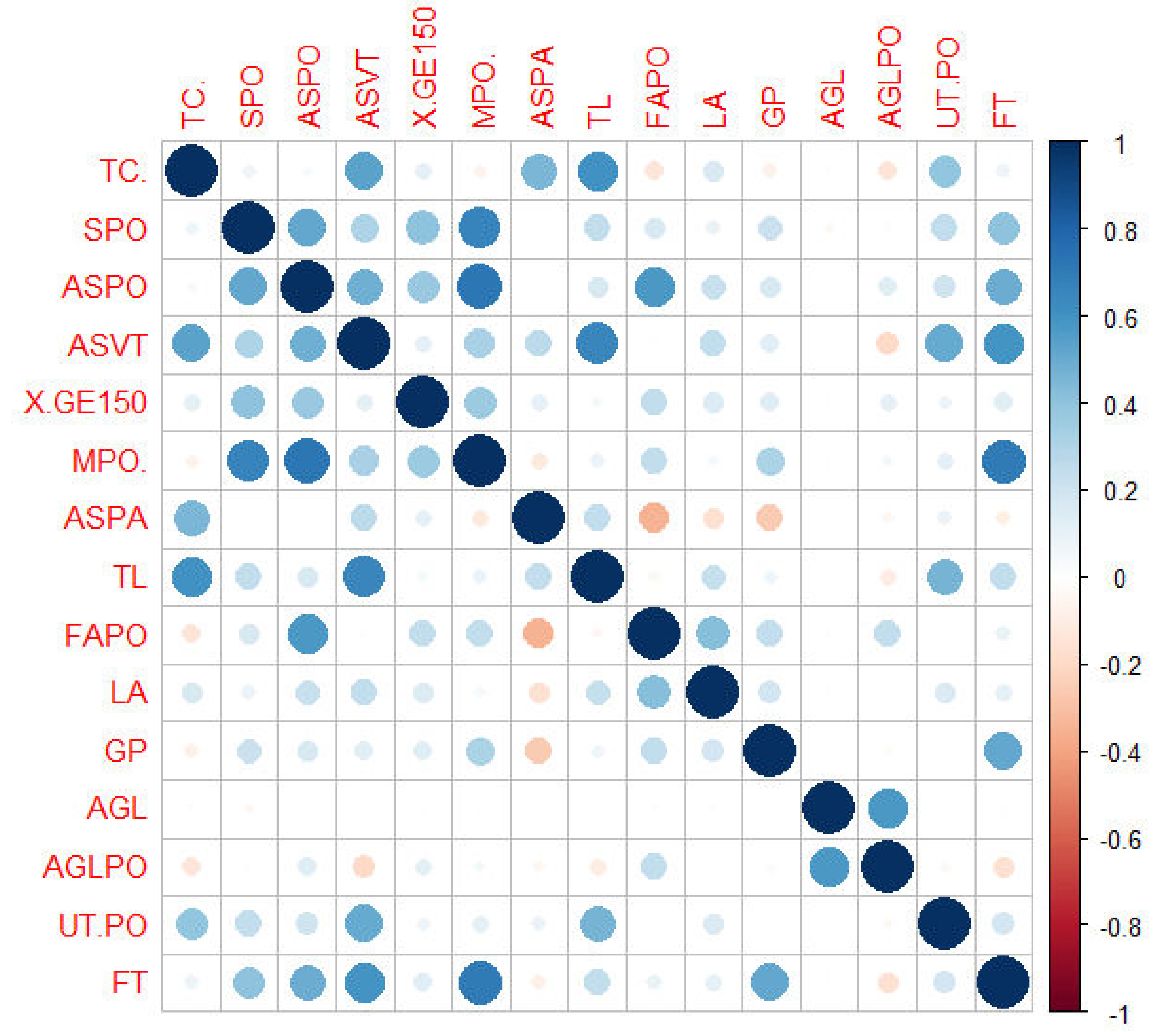
Cluster analysis works best when the variables have a low degree of correlation⁴⁹; we created a correlation matrix to measure the degree of correlation among the variables as our next step. Pearson correlation coefficients (rho) in absolute values between 0 and 0.2 are commonly interpreted as representing virtually no correlation among the variables; 0.2 to 0.5: weak correlation; 0.5 to 0.75: moderate correlation; 0.75 to 0.95: strong correlation; and 0.95 to 1: a nearly functional correlation. Table S1 presents the correlation matrix (please see the supplementary materials). We have also included a correlogram and heatmap (Figure 1) here. The blue scale represents a positive correlation between two variables, while the red represents a negative correlation. None of our variables displays a high degree of correlation with any other variable.

Next, we converted the 15 production potential variables into standardized Z-scores with zero mean and unit variance to give all variables equal weight in the cluster analysis.

In agglomerative hierarchical clustering, the algorithm considers each observation as a cluster itself [49]. Then, it merges the two closest clusters to form a new one and keeps repeating this process until it ends up with only one cluster. After the first two counties merge to form a multicounty cluster, there are three ways it can create new clusters:

• Combining two counties,
• Combining a county with a multicounty cluster formed at an earlier stage,
• Combining two multicounty clusters.

We used Ward’s minimum variance method for clustering in our analysis [50]. Ward’s minimum variance technique, a robust method, merges clusters to minimize the increase in the sum of the within-cluster deviation (distance) from the cluster means across all the variables [51]. The distance measure used in Ward’s method is squared Euclidean space, the sum of the squared differences between values of each clustering variable [52]. Other methods measure the distance directly, whereas Ward’s method analyzes the variance of clusters. Ward’s method is the most appropriate method for quantitative variables [50]. The hierarchical agglomerative analysis groups counties based on Euclidian distance measures, and then we use Ward’s minimum variance method to minimize intra-group dispersion and maximize inter-group separation [50].

In the first step, we calculated the distance for all possible pairs of observations and created the first cluster with the two nearest ones (most similar). For example, our first cluster included Autauga and Baldwin counties, Alabama. In the second step, we recalculated the distances where necessary, using the mean values of the newly formed cluster, and pooled the following two closest observations. The recalculation and merging process continued until step 2777 when all counties became one cluster.

We tried the partitioning method of clustering (k-means), the elbow method, density-based clustering, and the Silhouette method. However, those are all supervised learning methods; in other words, they work best when we know or have a better understanding of the optimal number of clusters. We decided on hierarchical clustering as our method for this study as we did not have a clear idea about the optimum number of clusters.

3. Results

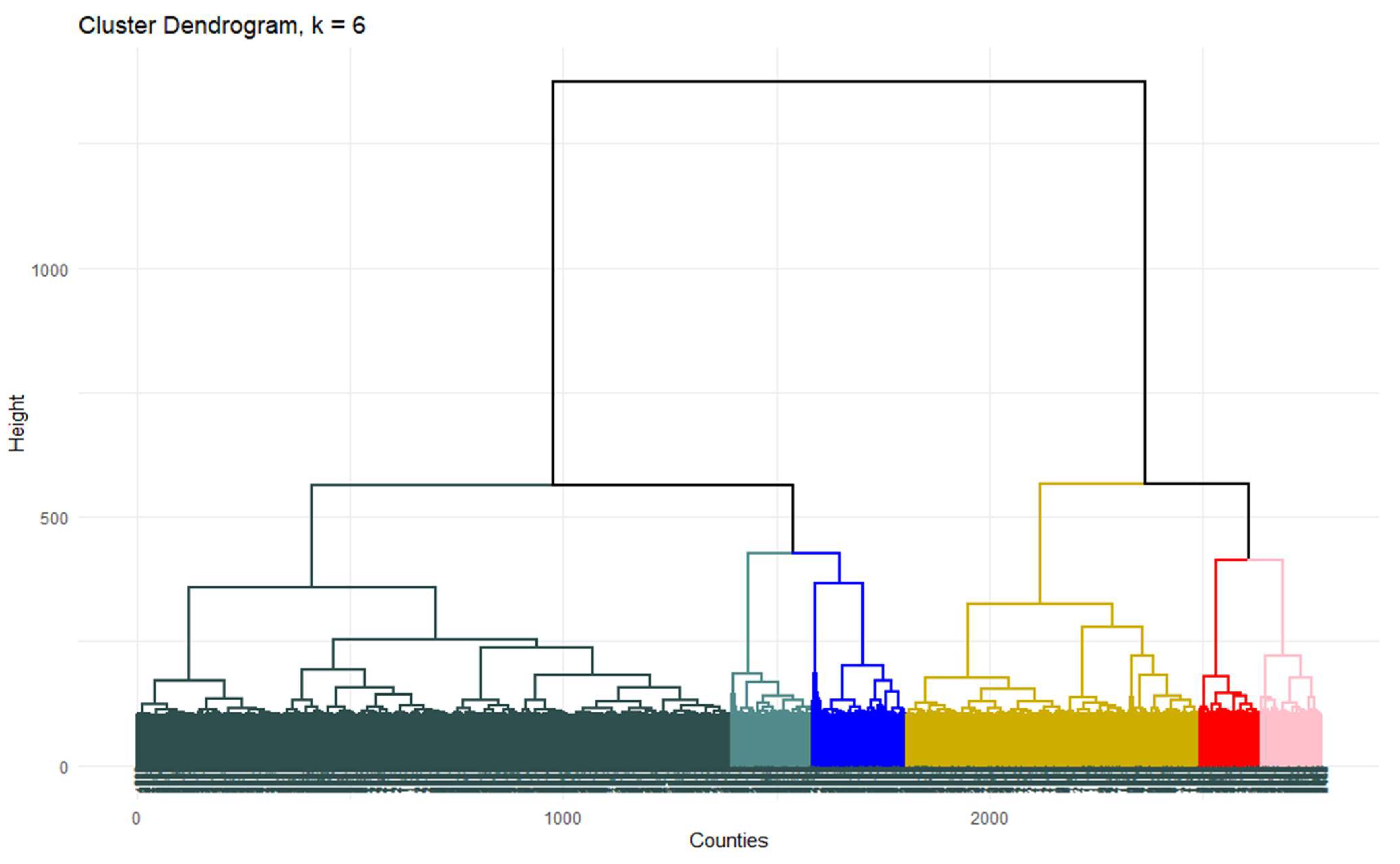
Hierarchical cluster analysis provides numerical information at each step of the clustering procedure. However, it does not have a definitive measure to determine when clustering has gone far enough. The method does not tell us the ultimate number of clusters for a particular research project. We, therefore, must turn to subjective measures. Determining the optimum number of clusters is our next step, as within-cluster heterogeneity increases as the number of clusters decreases. We used a dendrogram (Figure 2), a popular method in the literature, to determine our optimum number of clusters. As the dendrogram plots all the data points along the bottom, we see a black block along the bottom. We cannot read each data point separately when there are so many data points. We assigned each cluster to a group to analyze which county belongs to which cluster.

Looking at our dendrogram, we decided that three or four clusters would be a good choice. However, we should also keep our application in mind. We would probably want more than three clusters as we are trying to divide the entire contiguous US based on agricultural production potentials. Six or seven clusters emerged as the sweet spot. As the differences between clusters six and seven are minimal, we decided that six clusters provide meaningful county delineations for examining differential policy effects.

We analyzed each cluster on five attributes: farm size (four variables), farm assets (three variables), farm labor (two variables), farm output/performance (two variables), degree of mechanization (two variables), and government programs (two variables).

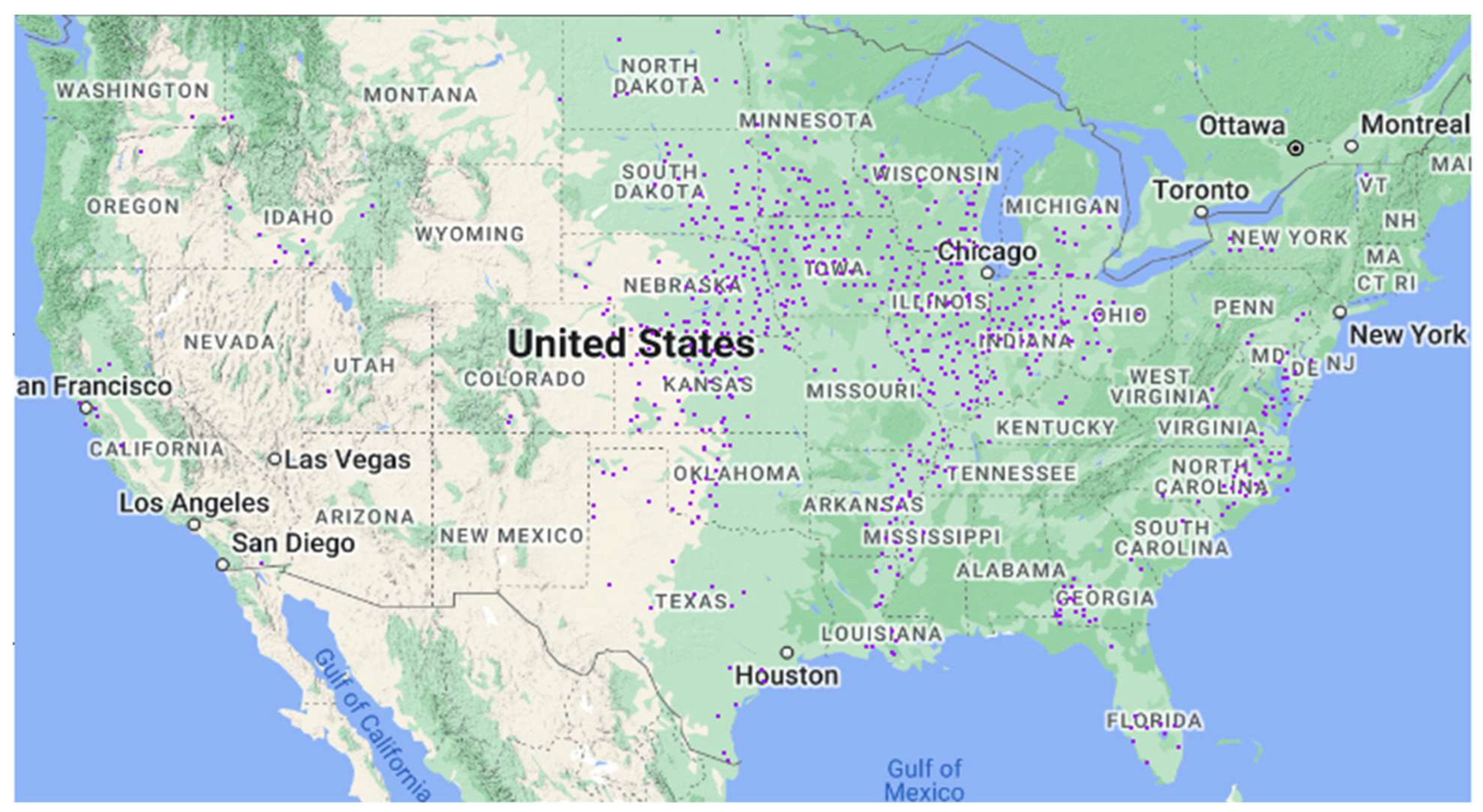
3.1. Cluster 1: Small Farm Majority

Fifty percent (1395) of the 2778 counties belong to this cluster. Cluster 1’s average farm size (269 acres) is smaller than the rest of the US (594 acres). Agricultural land per farm operation, excluding cropland, pastureland, and woodland (31 acres/operation), is lower than the national average of 44 acres per operation. If we only consider the agricultural land used for producing crops, cluster 1 has the second smallest farm area per operation among the six clusters. Our finding is also consistent with the total land area used per farm. Cluster 1 consists of small-scale farm operations.

The average per-farm investment in land and buildings (USD 612,165 per operation) is lower than the US average of USD 1.04 million per operation. The average asset value in this cluster is the lowest compared to the other five clusters. Asset value per acre is also the second lowest.

The degree of mechanization is the lowest in cluster 1. Machines used per operation (USD 57,000 per operation) are lower than the national average of USD 93,000. As a result, production and total consumption are also less in this cluster. Labor employment per farm is the smallest in this cluster. Around 24 percent of all commercial fertilizer and agricultural chemicals used on US farms are in this cluster. This might reflect an attempt to substitute low mechanization and low labor employment with more fertilizer and agri-chemicals. 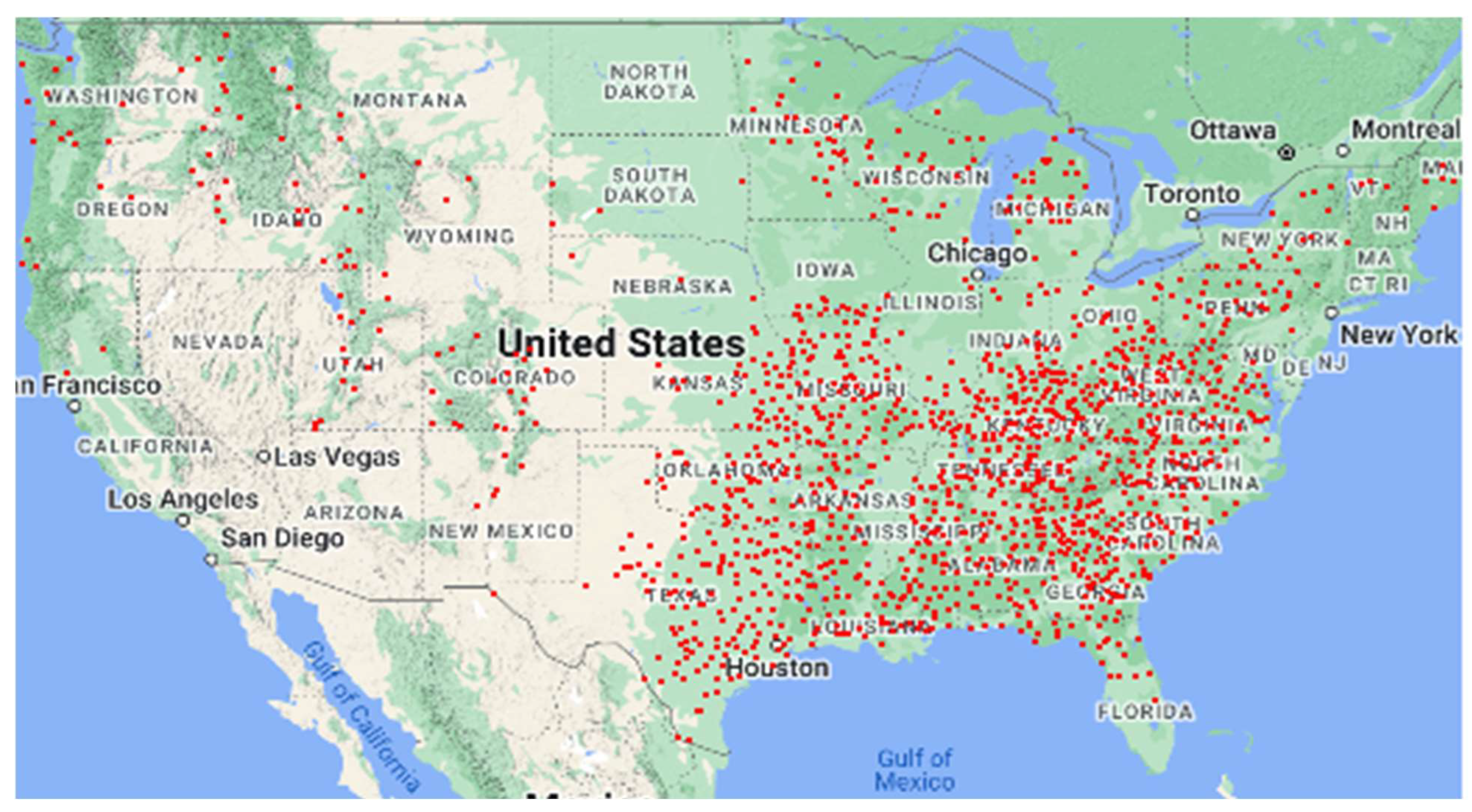Figure 3 shows the counties and states that are part of cluster 1.

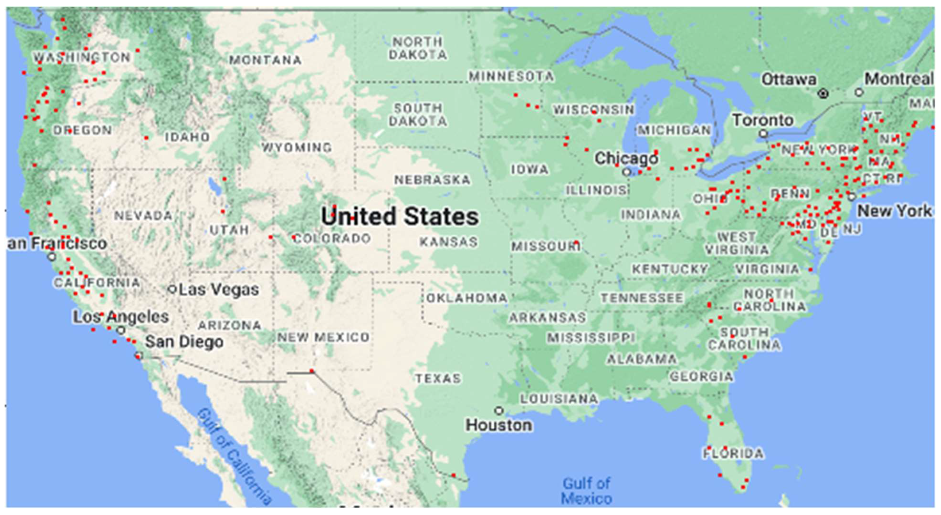
3.2. Cluster 2: Medium-Sized Farms

Cluster 2 demonstrates a very different picture from cluster 1. Cluster 2 consists of 190 counties from 30 states (7% of all counties). Average farm size is significantly larger than cluster 1, and agricultural land usage per farm is higher than the national average. Land usage per farm (167 acres per farm) is the highest in this cluster compared to the other subgroups. However, crop-producing farms are less prominent in this cluster.

Mean per-farm expenditure on land and buildings (USD 928,000 per operation) is close to the national average of USD 1.04 million per operation. The mean asset value in this cluster is the second lowest. Asset value per acre is also the least among the other five clusters.

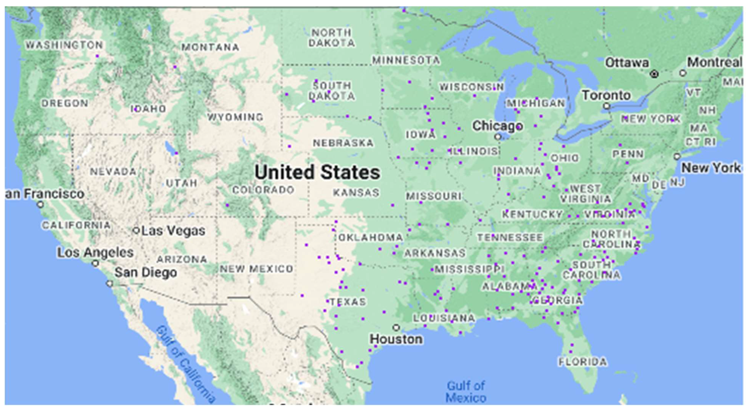
The intensity of mechanization is higher than cluster 1. Machines used per operation (USD 81,000 per operation) are close to the US average of USD 93,000. Consequently, both production and total consumption are higher than in cluster 1. Cluster 2 employs more labor per farm than cluster 1. Figure 4 shows the counties and states that are part of cluster 2.

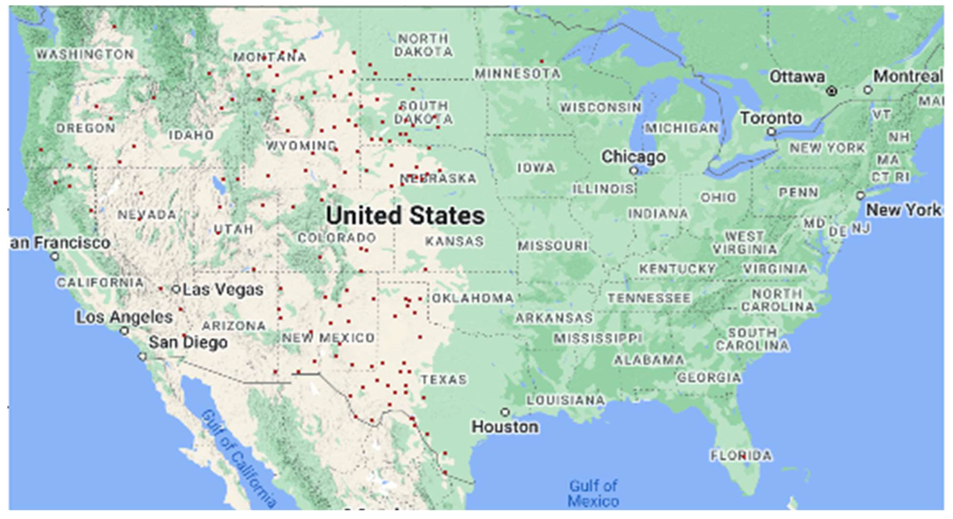
3.3. Cluster 3: Highly Mechanized Farms

Cluster 3 accommodates 690 counties from 37 states (25% of all counties). The average farm size in this cluster is similar to cluster 1. Both agricultural land usage (8700 acres per county) and agricultural land allocation per farm (36 acres) are very close to cluster 1. However, crop producers are more prominent in this cluster than in cluster 1.

The average per-farm spending on land and buildings (USD 1.5 million per operation) is higher than the national average of USD 1.04 million per operation. This cluster’s mean asset value and asset value per acre are the second highest.

The extent of mechanization is the second highest among all the clusters. Machines used per operation (USD 158,000 per operation) are well above the US average, while production and total consumption are the highest among all the clusters. Labor employment per farm is higher than cluster 1 but still the second lowest among all clusters, indicating substitution of machinery for labor. However, the percentage of hired workers who work more than 150 days per year is higher than in clusters 1 and 2. Figure 5 shows the counties and states that are part of cluster 3.

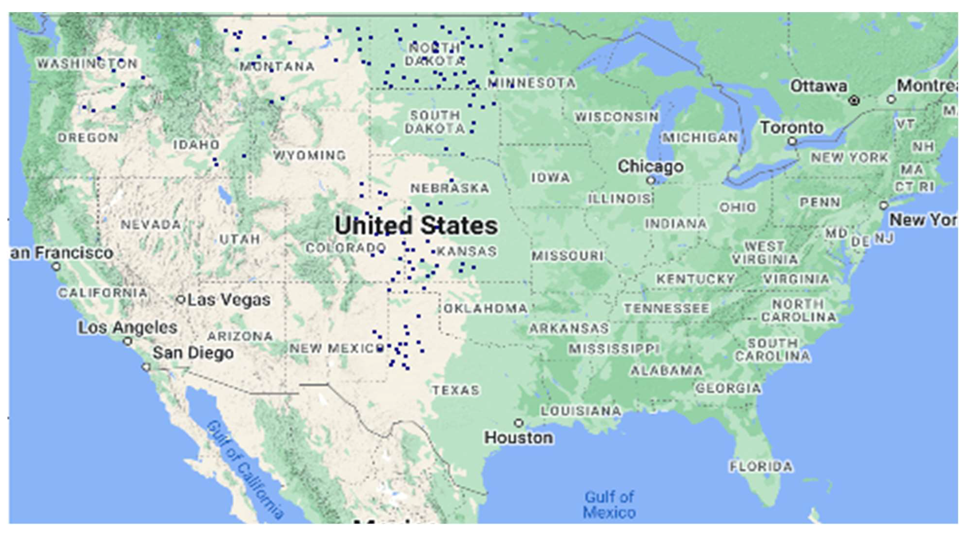
3.4. Cluster 4: Small, Labor-Intensive, High-Value Farms

Cluster 4 comprises 218 counties from 30 states (8% of all counties). Despite being one of the smaller clusters, cluster 4 exhibits intriguing characteristics. First, the asset value per acre and the average total asset value per farm are the highest among all the clusters. They are significantly higher than the national average.

Second, although these farms have very high values in terms of assets, the farms are not large by any means. Both land area per operation and farm area per operation are the lowest in this cluster. However, the total land used for agricultural activities is the highest among all the clusters. That means many small farms are operating in the counties that constitute this cluster.

This cluster employs the highest number of laborers (4000 workers per county versus the national average of 900 workers per county) by a large margin. However, since these farms are highly labor-intensive, they are not highly mechanized. This cluster has the second-lowest machine per operation expenditure among the six clusters. These farms are also the largest consumers of agricultural products. Figure 6 shows the counties and states that are part of cluster 4.

3.5. Cluster 5: Large Farms

Cluster 5 includes 142 counties from 18 states (5% of all counties) and is predominantly a cluster of large farms. For instance, the average asset value per operation is the largest in this cluster by a significant margin. Farm and land area per operation also show similar magnitude; they are the highest relative to the other clusters.

These farms are highly capital-intensive. The asset value per operation is the highest among all the clusters. However, the asset value to land area ratio is the lowest among the clusters and has a far lower value than the national average because of the heavy land usage.

The degree of mechanization in this cluster is not high. Cluster 5 stands in the third position relative to the others. A low degree of automation and low-level soil treatment (the lowest among all the clusters) impact this cluster’s productivity and agricultural consumption levels. Despite being a cluster of large farms, this cluster stands in the third position in agriculture sales and is marginally above the national level. Average farm consumption is also the lowest in this cluster.

Although farms in this cluster occupy large areas for agricultural activities, these farms do not employ a large labor force, as the total labor input is far below the national average (see Table S1). Figure 7 exhibits the counties and states that are part of cluster 5.

3.6. Cluster 6: The Most Productive Farms

Cluster 6 comprises 146 counties from 15 states (5% of all counties). Figure 7 exhibits the counties and states that are part of cluster 6. This cluster consists of the most mechanized and productive farms in the US. Machinery assets and sales per operation are the highest relative to the six clusters. Cluster 6 also contains the most treated agricultural land in the US; the average per county-treated land is above the national average. The high degree of mechanization, government spending on infrastructure development, and good soil practice have made this cluster the most productive agricultural region.

Farms in this cluster are not large. The farm size variables show modest values; however, these farms are not heavily capital-intensive. The total asset value and the average asset per farm are marginally above the national average. The labor usage is well below the national average and stands second lowest among all the clusters. Figure 8 exhibits the counties and states that are part of cluster 6. Table S1 summarizes the differences in critical variables between clusters.

4. Discussion and Conclusions

The US agricultural sector is diverse in its enterprises, resources, and interactions with the rest of the economy. The farm sector consists of more than 2 million farms with production factors ranging from a few hundred dollars of investment to assets worth several million dollars. Farms produce a wide range of commodities and interact with non-farm labor markets, ranging from operators mainly working off the farm to operators depending on the farm for all income.

For over a century, economists have attempted to identify patterns in US farming that further the comprehension of differences in the economic performance of farms and the economic well-being of farm households. The United States Department of Agriculture (USDA) has divided the country into eight Farm Resource Regions. They derived the Farm Resource Regions based on four analyses: a cluster analysis of US farm characteristics1, their Old Farm Production Regions, USDA’s Land Resource Regions, and the National Agricultural Statistics Service (NASS) Crop Reporting Districts. However, recent studies need to catch up. Our paper contributes to this critical but outdated body of literature.

The goal of this study was to identify the patterns of counties that appear when we analyze the farm sector characteristics without considering state lines or USDA Farm Resource Region boundaries. The goals of agricultural policies have evolved over the past few decades, incorporating production, environmental, rural, social, and energy usage questions. Identifying farm sector diversity using advanced methodologies, like clustering analysis, is crucial for policy analysis.

We applied agglomerative hierarchical cluster analysis with county-level data to distinguish US counties into six relatively homogeneous clusters concerning production potentials. The six clusters are: Small Farm Majority (cluster 1), farms with low values of land, buildings, and machinery per farm; Medium-Sized Farms (cluster 2), farms with asset values per farm that are close to the US average; Highly Mechanized Farms (cluster 3), farms with high values of land, buildings, and machinery per farm but low levels of labor per farm; Small, Labor-Intensive, High-Value Farms (cluster 4), farms with high values of labor and assets per farm but small values of land area per farm; Large Farms (cluster 5), farms with high levels of assets and land per farm, but low levels of assets per acre; and The Most Productive Farms (cluster 6), with high levels of machinery and sales per farm, medium levels of land area per farm, and low levels of labor per farm.

One interesting finding is that the difference between clusters in the scale of farm operations is more than a simple small-medium-large distinction. Counties in the same cluster can have farms that are large in scale on some measures but medium or small in scale on others. For example, the high-value farms in cluster (4) are large in scale as measured by labor and assets per farm, but small as measured by land area per farm. Another example is the most productive farms cluster (6), comprising farms that are large in scale as measured by machinery per farm but small in scale as measured by labor per farm.

Each of our six clusters represents a set of production factors that is relatively homogeneous for five dimensions: farm size, farm assets, farm labor, farm output, degree of mechanization, and government programs. At the same time, because the counties are often spatially separated within a cluster, this clustering can help us understand the impact of a market or policy change across the contiguous United States.

We can identify agricultural sector heterogeneity by studying the attributes of farms within a cluster or by comparing the differences in characteristics across clusters. Understanding the heterogeneity or homogeneity of US agriculture can increase our understanding of the effects of agricultural policies and programs on various types of farms within the industry. Such an understanding can also help explain differences in responses within the US agricultural sector to national and global economic forces. Carrying out a policy or market analysis is beyond the scope of this article, but the results here can help lay the foundation for such an analysis.

One limitation of our study is that clustering, as a means of simplifying farm complexity into a small number of distinct, relatively homogenous clusters, is silent on heterogeneity within each cluster. A way to extend our clustering method would be to statistically analyze differences in farm characteristics within and between clusters.

Another limitation is that we have attempted to identify homogeneity of different types of farms at the county level. This study could be extended by doing a farm-level analysis, i.e., clustering similar types of farms based on their production potential regardless of county.