Motion-Control Strategy for a Heavy-Duty Transport Hexapod Robot on Rugged Agricultural Terrains

Abstract

Legged agricultural transportation robots are efficient tools that can autonomously transport goods over agricultural terrain, and their introduction helps to improve the efficiency and quality of agricultural production. Their effectiveness depends on their adaptability to different environmental conditions, which is especially true for heavy-duty robots that exert ground forces. Therefore, this study proposes a motion-control strategy for a heavy-duty transport hexapod robot. Two critical tasks were accomplished in this paper: (1) estimating the support surface angle based on the robot’s foot position and body posture, and accordingly determining the motion constraint conditions on this support surface and the body posture based on energy optimization; (2) proposing an adaptive fuzzy impedance algorithm for real-time force–position composite control for adjusting foot position, in order to reduce the steady-state force tracking error caused by terrain stiffness, thus ensuring body stability through tracking of variable foot-end forces. An element of hardware in the loop control platform for a 3.55-ton device was designed and compared with the current popular force-control methods under different external contact terrains. The results show that the proposed control method can effectively reduce force errors, establish support forces faster on less-stiff environments, and reduce the torso tilt during phase switching.

1. Introduction

As robots continue to expand their role within agricultural settings, there has been extensive research on agricultural robots [1]. The primary research focus has largely been on wheeled and tracked mobile robots [2]. These robots accomplish various tasks through the integration of multiple sensor technologies such as computer vision, radar, GPS, and audio signals [3,4]. In agricultural activities, most of which are on unstructured terrain often accompanied by rugged and steep road surfaces, compared with other types of robots, the main advantage of legged robots given the unstructured terrain is their excellent terrain adaptability, together with the corresponding top-loading platforms, which can play a good role in the development of agricultural production [5]. On an unstructured terrain, studying the posture of legged robots is crucial for their adaptation to the environment. Adjusting their posture to suit the terrain can improve their adaptation ability. To achieve this, Song et al. [6] proposed a quasi-static climbing gait that enhances the movement of a robot on complex terrain. This gait enables the robot to climb steps that are 3.9 times the length of its legs. Lee [7] conducted a study on a hexapod adaptive suspension vehicle (ASV) by analyzing the robot’s body posture on various inclines. A hexapod robot can traverse surfaces at different inclination levels by adjusting its torso height and posture. However, owing to the inherent variability in the end position of the foot and the susceptibility of legged robots to external environmental factors, controlling their motion on unstructured terrain has become a subject of extensive research [8,9]. A hexapod robot can traverse surfaces at different inclination levels by adjusting its torso height and posture. Boston Dynamics [10] developed the Little Dog, a four-legged robot that optimizes its stance to maximize the movement space while ensuring that its torso does not collide with the ground. However, achieving energy efficiency is challenging for legged robots with high loads [11]. A poor distribution of foot forces can lead to energy wastage, out-of-range joint moments, and even mechanical structural damage. Therefore, rational movement is necessary to reduce energy consumption.

Impedance control [12] is a widely used robotic control technique that adjusts the force-feedback error based on the relationship between the contact force and the robot’s foot-end position. Zhu [13,14] proposed a hybrid sliding film control algorithm for a hydraulic quadrupedal robot based on impedance control which resulted in improved control accuracy. Subsequently, Wang [15] developed a whole-body control architecture that included impedance control to reduce the impact of contact between the legs of a six-legged robot and the environment, thus enabling smoother contact. However, conventional impedance control models are prone to steady-state errors during force tracking owing to uncertainties associated with the environmental parameters of the terrain [16]. Several approaches have been explored to mitigate such errors, with some focusing on controlling the model reference [17,18,19,20,21]. For instance, Roveda [17] proposed a method to estimate the environmental stiffness and adjust the controller gain to compensate for unknown environmental stiffness, whereas Deng [18] employed an extended Kalman filter to estimate force-tracking errors. Wang [20] introduced an impedance-estimation method for estimating contact in an uncalibrated environment. However, none of these methods demonstrated satisfactory force-tracking performance under time-varying forces. Furthermore, because the aforementioned methods rely on the estimation of environmental impedance parameters, they inevitably incur errors when addressing complex and variable environments.

Researchers have explored the use of variable impedance control methods based on reinforcement learning and optimization-based approaches. Chao and Yang estimated human stiffness dynamics using a dynamic motion primitive (DMP) [22] and a Markov model with Gaussian mixed regression [23], respectively. Zhang, et al. [24] proposed a convolutional neural network (CNN) supervised-learning method to calibrate the force estimation algorithm. Modares [25] transformed the optimal parameter search problem for impedance models into a linear quadratic regulator (LQR) problem. However, these methods require extensive data collection or calculations that negatively affect the real-time tracking of the time-varying forces of a robot.

In conclusion, the current impedance-control techniques for legged robots face difficulties in achieving the desired tracking of time-varying forces in complex environments, particularly when considering real-time performance. Previous studies have demonstrated that adaptive architectures provide high robustness in uncertain dynamic systems [26,27,28]. Therefore, an adaptive motion strategy was proposed for complex terrains by adapting a robot torso pose to the instant terrain considering motion constraints and energy-optimal conditions under the support surface of the terrain. Subsequently, positional maintenance was achieved through adaptive fuzzy impedance control as follows:

(1)

A terrain-adaptive motion strategy was proposed, one which improves the stability of the robot’s motion process by estimating the angle of the support surface on the current terrain, setting up corresponding reaction mechanisms, and analyzing the energy consumption of different positions on the same support surface to select the most energy-efficient motion posture.

(2)

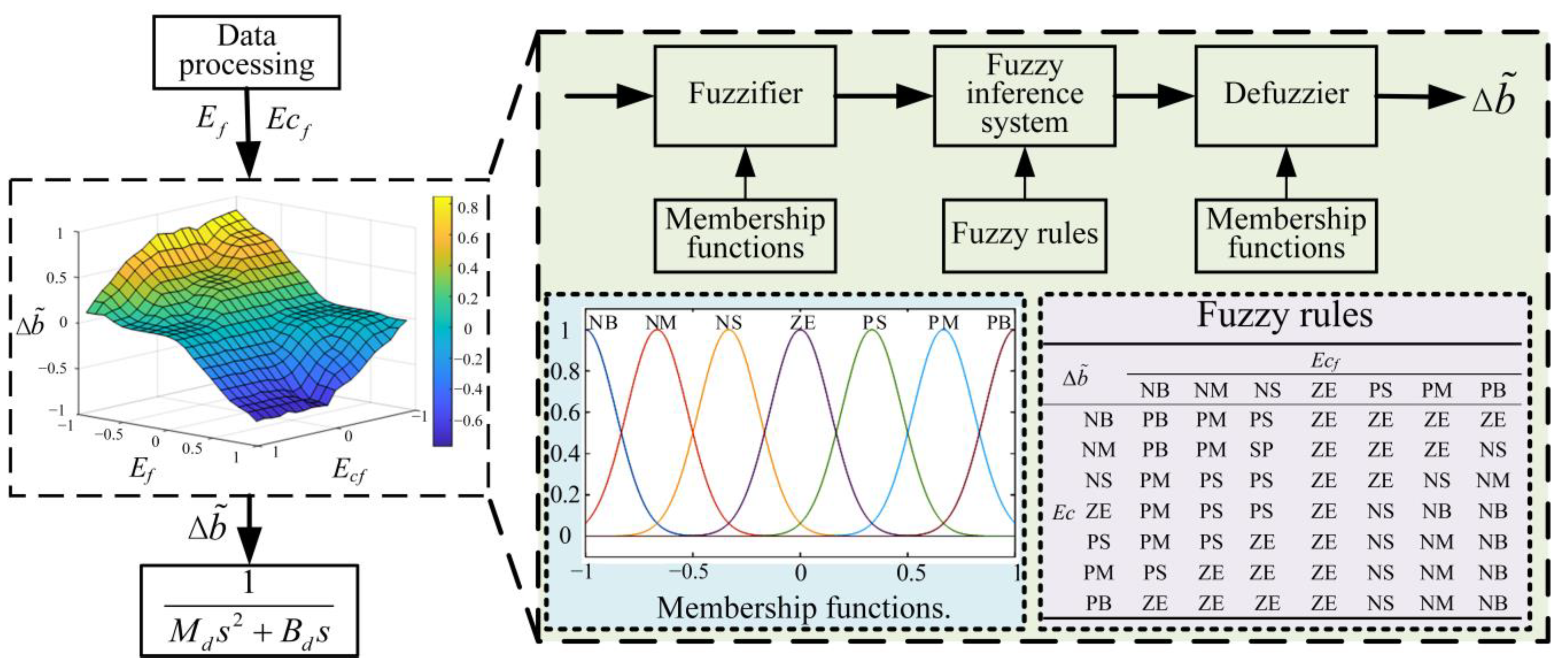
The contact force dynamics were used to describe the influence of parameters such as environmental stiffness on the impedance model, and an adaptive fuzzy impedance control strategy based on force–position control was proposed to mitigate the impact of the external environment on impedance control.

(3)

The efficacy of the proposed control strategy in complex environments was verified through comparative experiments.

This paper is organized as follows: In Section 2, we present the motion model and terrain estimation algorithm for an agricultural transportation robot with terrain adaptation on the rugged terrains of agriculture. Section 3 presents an adaptive impedance system that includes terrain-adaptive control and fuzzy parameter-adjustment methods. In Section 4, we present an experimental validation of the proposed method. Finally, Section 5 concludes the study.

2. Terrain-Adaptive Methods

The hexapod robot structure depicted in Figure 1 consists of two main components: the torso and the legs. The legs and torso’s mounting positions are elliptically distributed, and each leg comprises a hip joint, thigh, and shin connected by a rotating pair between two adjacent segments, and a calf and foot-end connected by a ball hinge. An electro-hydraulic control system was selected as the transmission system, and integrated with low-impact motion trajectory planning to complete the trajectory planning. The robot can carry four people and can traverse over 1 m obstacles and across 1.2 m trenches, as well as achieve 40° longitudinal climbing and 30° lateral climbing. The robot movement includes two phases: swing and support. During the swing phase, the legs of the robot can be treated as single-leg tandem mechanisms, whereas during the support phase, the legs and the torso form parallel mechanisms. The position of the robot changes when it switches between the two phases of motion. Defined based on the established coordinate system shown in Figure 1, the coordinate transformation matrix formula for joint i can be obtained using the D-H parameter method, and the D-H parameters of the robot’s single leg are shown in

Table 1. D-H parameter of the leg.

	${\mathit{L}}_{\mathit{i}}$	${\mathit{d}}_{\mathit{i}}$	${\mathit{\alpha }}_{\mathit{i}}$	${\mathit{\theta }}_{\mathit{i}}$
Hip joint	$l_1$	0	$\pi /2$	${\theta }_1$
Thigh	$l_2$	0	0	${\theta }_2$
Shin	$l_3$	0	0	${\theta }_3$

.

The transformation matrix of the foot-end of leg j of the hexapod robot relative to the torso coordinate system is expressed as:

$$\left[\begin{array}{c}{}^{\mathrm{C}}{x}_{j3}\\ {}^{\mathrm{C}}{y}_{j3}\\ {}^{\mathrm{C}}{z}_{j3}\end{array}\right]=\left[\begin{array}{c}{l}_{j0}+l_{1}c{\theta }_1+l_{2}c{\theta }_{1}c{\theta }_2+l_{3}c{\theta }_{1}c({\theta }_2+{\theta }_3)\\ b_{j0}+l_{1}s{\theta }_1+l_{2}s{\theta }_{1}c{\theta }_2+l_{3}s{\theta }_{1}c({\theta }_2+{\theta }_3)\\ z_{j0}-l_{2}s{\theta }_2-l_{3}s({\theta }_2+{\theta }_3)\end{array}\right]$$

(1)

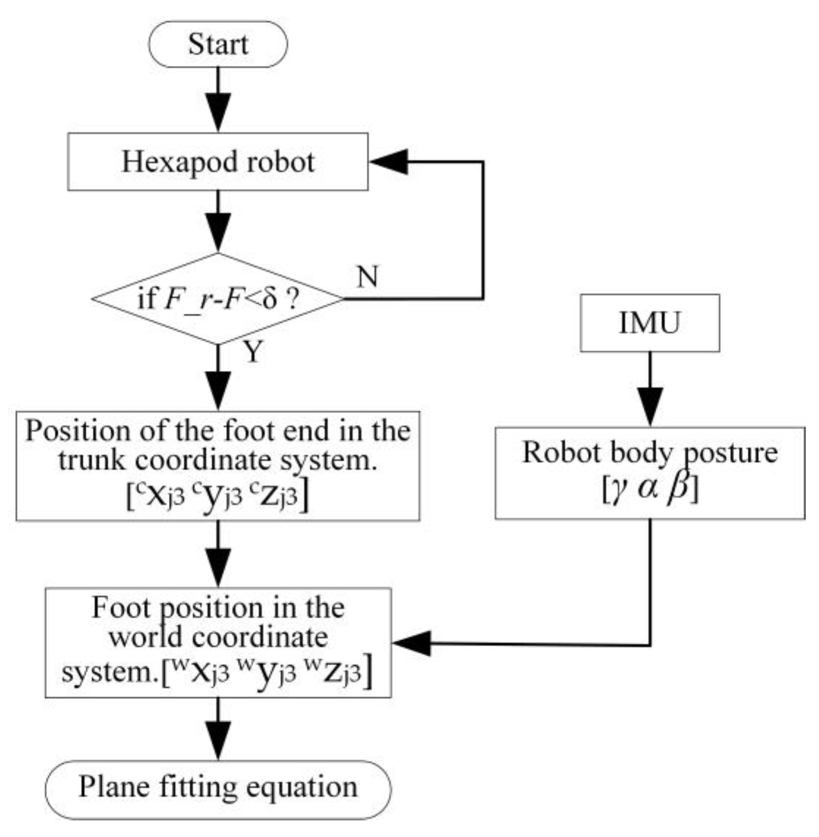
2.1. Terrain Estimation

The overall terrain-perception process of the robot is as depicted in Figure 2. Initially, the controller detects the force signal from the foot-end force sensor, determining whether the foot-end has reached the support state based on whether the force exceeds the stable force threshold for foot grounding. Subsequently, the position of the foot-end in the support state relative to the body coordinate system is calculated through the displacement sensor of the hydraulic cylinder. The position of the supporting leg end relative to the body coordinate system is then recorded and, based on the body posture angle gathered by the IMU, the position information of the foot-end under the body coordinate system is transformed into the world coordinate system. Lastly, using the foot-end information under the world coordinate system, a plane fitting method is applied to fit the terrain information, thereby estimating the local terrain information where the hexapod robot is currently situated.

To simplify the calculation of terrain estimates, a reference coordinate system, denoted by O_B-X_BY_BZ_B, was established to quantitatively convert the foot-end position information when characterizing the local terrain. As illustrated in Figure 3, Origin B of the reference coordinate system c coincides with Origin C of the torso coordinate system O_C-X_CY_CZ_C, whereas its x-, y-, and z-axis directions align with those of the reference coordinate system O_W-X_WY_WZ_W. The positional transformation of the torso is referenced to the world coordinate system O_B-X_BY_BZ_B, and the transformation matrix of the torso coordinate system with respect to the world coordinate system is given by Equation (2).

$${}^{\mathrm{B}}A{}_{\mathrm{C}}=\left[\begin{array}{cccc}c\gamma c\alpha & c\gamma s\alpha s\beta -s\gamma c\beta & c\gamma s\alpha c\beta +s\gamma s\beta & 0\\ s\gamma c\alpha & s\gamma s\alpha s\beta +c\gamma c\beta & s\gamma s\alpha c\beta -c\gamma s\beta & 0\\ -s\alpha & c\alpha s\beta & c\alpha c\beta & 0\\ 0& 0& 0& 1\end{array}\right]$$

(2)

where γ, α, and β denote the yaw, pitch, and roll angles, respectively, of the torso coordinate system in the world coordinate system, as measured by the inertial measurement unit (IMU).

For any leg of the six-legged robot, the coordinates of the foot-end position relative to the world coordinate system can be derived using Equation (3).

$$\left[\begin{array}{c}\begin{array}{c}{}^{\mathrm{B}}{x}_{j3}\\ {}^{\mathrm{B}}{y}_{j3}\\ {}^{\mathrm{B}}{z}_{j3}\end{array}\\ 1\end{array}\right]={}^{\mathrm{B}}A{}_{\mathrm{C}}\left[\begin{array}{c}\begin{array}{c}{}^{\mathrm{C}}{x}_{j3}\\ {}^{\mathrm{C}}{y}_{j3}\\ {}^{\mathrm{C}}{z}_{j3}\end{array}\\ 1\end{array}\right]$$

(3)

The location information of the support foot was regarded as the terrain location feature point in the terrain information, and a single-plane fitting method was employed to fit these terrain location feature points. The primary plane-fitting equation was as follows:

$$z=f(x,y)=a_0+a_{1}x+a_{2}y$$

(4)

where a₀, a₁, and a₂ represent the coefficients of the plane equation.

The coefficients of the primary plane expression were determined using the least-squares method based on the coordinates of the foot-end position of the hexapod robot in the support phase. The solution equation is as follows:

$$\left[\begin{array}{l}{a}_0\\ a_1\\ a_2\end{array}\right]=(A^{T}A)A^{T}Z$$

(5)

where A = [1 ^Bx_sj3 ^By_sj3], Z = [^Bz_sj3], s_j3 is the number of legs in a supported state, and the number of legs in different gaits varies, and is obtained based on trajectory planning.

By segmenting the terrain slope based on the ground-pitch and side-inclination angles, an equation for estimating the slope of an unexplored terrain was obtained:

$$\left\{\begin{array}{l}{\phi }_x=\arctan (a_2)\\ {\phi }_y=\arctan (a_1)\end{array}\right.$$

(6)

2.2. Attitude Adaptive Adjustment

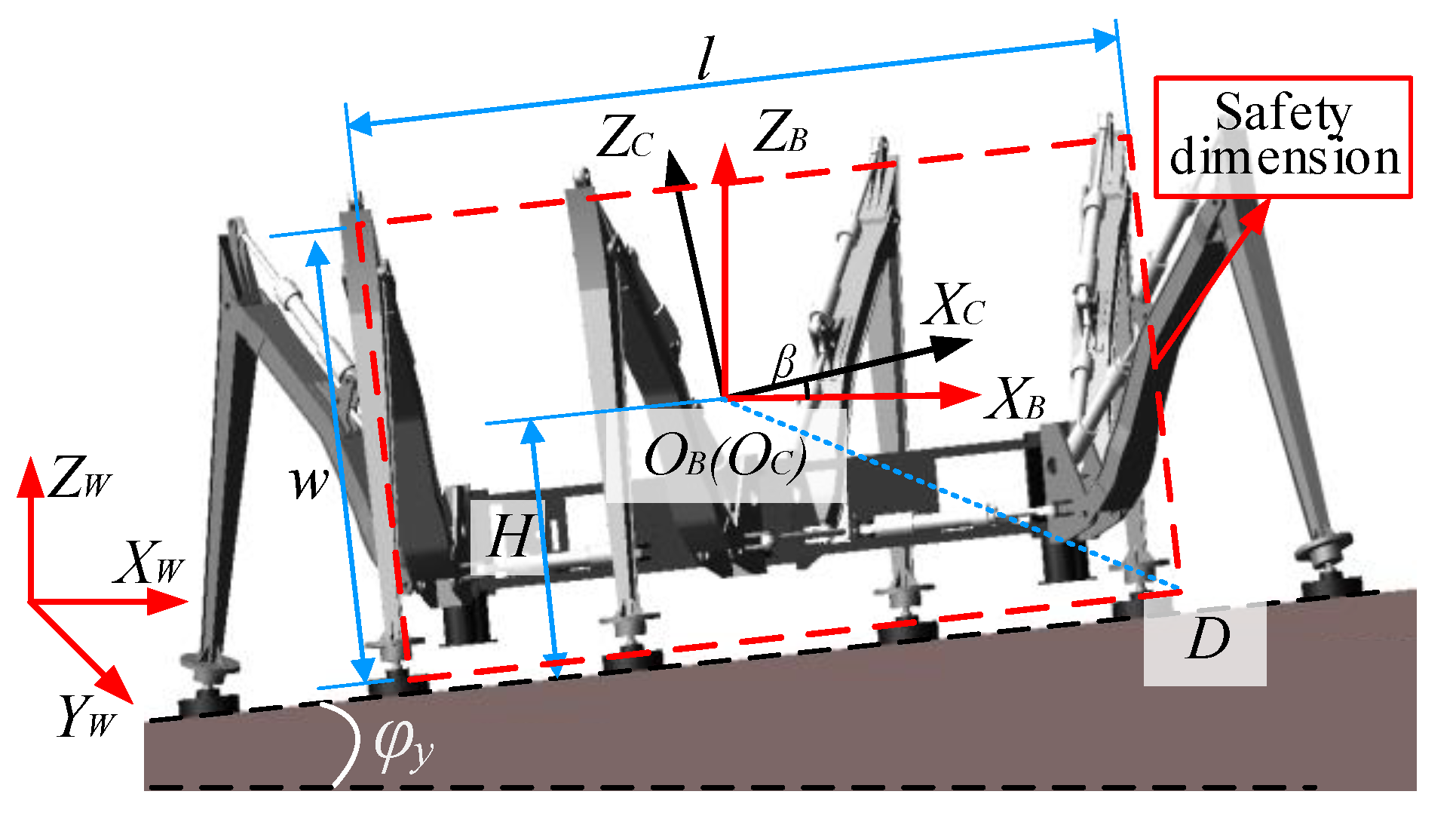
2.2.1. Torso Safety Dimension Constraints

The robot must avoid collisions between its torso and the environment when traversing complex terrain. Thus, when the terrain slope varies significantly, it is necessary to establish a geometric constraint between the robot torso safety zone dimensions and the terrain slope. The solid box in Figure 3 represents the torso profile of the robot, while the dashed line represents the minimum allowable torso safety zone dimensions for a six-legged robot with torso length l height w, and width h. The ground-pitch and ground-side-tilt angles, φ_x and φ_y, were estimated.

To ensure that the torso is not interfered with by the terrain, point D must remain above the slope throughout the motion. The torso attitude angle and geometric constraints facilitated the determination of the coordinates of point D relative to the reference coordinate system O_W-X_WY_WZ_W.

$$\left\{\begin{array}{l}{}^{\mathrm{B}}{x}_D=\frac{l}{2}\cos \alpha -\frac{w}{2}\sin \alpha \\ {}^{\mathrm{B}}{y}_D=\frac{h}{2}\\ {}^{\mathrm{B}}{z}_D=\frac{l}{2}\sin \alpha -\frac{w}{2}\cos \alpha \end{array}\right.$$

(7)

Substituting the coordinates from Equation (7) into Equation (4) yields the constraint equation for a safe torso zone size.

$$a_0+(\frac{l}{2}c\alpha -\frac{w}{2}s\alpha )\tan {\phi }_y+\frac{a_{2}h}{2}-(\frac{l}{2}s\alpha -\frac{w}{2}c\alpha )\tan {\phi }_x<0$$

(8)

$$a_0=\frac{H}{\sqrt{a_1{}^2+a_2{}^2+1}}$$

(9)

Thus, when the torso-pitch, cross-roll, ground-pitch, and ground-side-tilt angles are β, α, φ_x, and φ_y, respectively, the constraint relationship between the torso position and the terrain environment can be obtained by combining Equations (6) and (9) as follows:

$$(\frac{l}{2}c\alpha +\frac{w}{2}s\alpha s\beta +\frac{h}{2}s\alpha c\beta )\tan {\phi }_y-\frac{l}{2}s\alpha -\frac{h}{2}c\alpha s\beta +\frac{H}{\sqrt{{(\tan {\phi }_y)}^2+{(\tan {\phi }_x)}^2+1}}+(\frac{w}{2}c\beta -\frac{h}{2}c\beta )\tan {\phi }_x<0$$

(10)

The robot needs to adjust its torso posture to change its direction of motion when there are obstacles in the motion’s path. An RGB-D camera is installed directly in front of the robot’s centroid in the x direction. The distance between the obstacle and the robot is calculated based on depth information when the target obstacle is detected. Then, by adjusting the posture of the torso, obstacle avoidance actions are performed in advance, as shown in Figure 4a. R is the safe distance to adjust the yaw angle of the torso. The calculation formula for torso deflection angle $\delta$ is as follows:

$$\delta =\arccos \frac{b_r/2+w_2/2}{\sqrt{x_{dr}{}^2+y_{dr}{}^2}}-\arctan \frac{y_{dr}}{x_{dr}+l}$$

(11)

where x_dr and y_dr are the positions of obstacles relative to camera coordinates, and their border dimensions are b_r and h_r; w₂ is the safe size of the robot’s zone, and l₂ is the distance from the camera to the centroid.

2.2.2. Stability Constraints on Inclined Terrain

This study proposes a normalized energy stability margin (NESM) as a criterion for assessing the stability of a robot on an inclined terrain. The NESM method considers the center of mass of the robot, the locations of the support feet’s ends, and the slope of the terrain.

As shown in Figure 4b, the center-of-mass location in the reference coordinate system is denoted by ^BO_G (^Bx_G, ^By_G, ^Bz_G). The adjacent foot-end points of the robot for leg-end positions leg1 and leg3 are denoted as A₁ (^Bx₁₃, ^By₁₃, ^Bz₁₃) and A₃ (^Bx₃₃, ^By₃₃, ^Bz₃₃), respectively. The point ^SO_G is the projection of the center-of-mass on the slope surface S, and ^BO_G forms a vertical line with Line A₁A₃. The intersection point of ^BO_G and the vertical line is N (^Bx_N, ^By_N, ^Bz_N). Point ^BO_Gh is the highest point that ^BO_G can reach by rotating around the support edge A₁A₃. The angle between ^BO_Gh and the horizontal plane is denoted as θ. The angle between the support boundary c and the horizontal plane is denoted as α, and M is the intersection point of the perpendicular line from the center-of-mass ^BO_G to the straight line ^BO_GhN.

The expression for the line A₁A₃ can be found from the following linear formula:

$$\frac{x-{}^{\mathrm{B}}x{}_{13}}{{}^{\mathrm{B}}{x}_{33}-{}^{\mathrm{B}}x{}_{13}}=\frac{y-{}^{\mathrm{B}}y{}_{13}}{{}^{\mathrm{B}}{y}_{33}-{}^{\mathrm{B}}y{}_{13}}=\frac{z-{}^{\mathrm{B}}z{}_{13}}{{}^{\mathrm{B}}{z}_{33}-{}^{\mathrm{B}}z{}_{13}}$$

(12)

The distance from point ^BO_G to line A₁A₃ was calculated using the following formula:

$$D_i=\frac{\sqrt{P+K+W}}{\sqrt{Q}}$$

(13)

where $W=\left|\begin{array}{cc}{}^{\mathrm{B}}{z}_G-{}^{\mathrm{B}}z{}_{13}& {}^{\mathrm{B}}{x}_G-{}^{\mathrm{B}}x{}_{13}\\ {}^{\mathrm{B}}{z}_{33}-{}^{\mathrm{B}}z{}_{13}& {}^{\mathrm{B}}{x}_{33}-{}^{\mathrm{B}}z{}_{13}\end{array}\right|$; $K=\left|\begin{array}{cc}{}^{\mathrm{B}}y{}_G-{}^{\mathrm{B}}y{}_{13}& {}^{\mathrm{B}}z{}_G-{}^{\mathrm{B}}z{}_{13}\\ {}^{\mathrm{B}}y{}_{33}-{}^{\mathrm{B}}y{}_{13}& {}^{\mathrm{B}}z{}_{33}-{}^{\mathrm{B}}z{}_{13}\end{array}\right|$; and $P=\left|\begin{array}{cc}{}^{\mathrm{B}}x{}_G-{}^{\mathrm{B}}x{}_{13}& {}^{\mathrm{B}}y{}_G-{}^{\mathrm{B}}y{}_{13}\\ {}^{\mathrm{B}}x{}_{33}-{}^{\mathrm{B}}x{}_{13}& {}^{\mathrm{B}}y{}_{33}-{}^{\mathrm{B}}y{}_{13}\end{array}\right|$.

The normal vector of the vertical plane A₁A₃ ^BO_Gh passing through the straight-line c is as follows:

$$n_{{\mathrm{A}}_1{\mathrm{A}}_3{}^{\mathrm{B}}{O}_{\mathrm{Gh}}}=\left[\begin{array}{ccc}i& j& k\\ {}^{\mathrm{B}}x{}_{\mathrm{G}}-{}^{\mathrm{B}}x{}_{13}& {}^{\mathrm{B}}y{}_{\mathrm{G}}-{}^{\mathrm{B}}y{}_{13}& {}^{\mathrm{B}}z{}_G-{}^{\mathrm{B}}z{}_{13}\\ 0& 0& 1\end{array}\right]$$

(14)

The vector of line ${}^{\mathrm{B}}O{}_{\mathrm{G}}N$ can be found when the coordinates of N and ^BO_G are known.

$$l_{{}^{\mathrm{B}}O{}_G\mathrm{N}}=({}^{\mathrm{B}}x{}_{\mathrm{N}}-{}^{\mathrm{B}}x{}_{{}^{\mathrm{B}}O{}_{\mathrm{G}}},{}^{\mathrm{B}}y{}_{\mathrm{N}}-{}^{\mathrm{B}}y{}_{{}^{\mathrm{B}}O{}_{\mathrm{G}}},{}^{\mathrm{B}}z{}_{\mathrm{N}}-{}^{\mathrm{B}}z{}_{{}^{\mathrm{B}}O{}_{\mathrm{G}}})$$

(15)

$${\zeta }_i=\arcsin (\frac{l_{{}^{\mathrm{B}}O{}_G\mathrm{N}}\cdot n_{{\mathrm{A}}_1{\mathrm{A}}_3{}^{\mathrm{B}}O{}_{\mathrm{Gh}}}}{\left|l_{{}^{\mathrm{B}}O{}_{\mathrm{G}}N}\right|\cdot \left|n_{{\mathrm{A}}_1{\mathrm{A}}_3{}^{\mathrm{B}}O{}_{\mathrm{Gh}}}\right|})$$

(16)

The angle between A₁A₃ and the horizontal plane ξ_i can be determined similarly. The degree of stability with A₁A₃ as the boundary condition can be calculated from the definition of NESM, as follows:

$$E_i=D_i(1-\cos {\zeta }_i)\cos {\xi }_i$$

(17)

Based on the definition of NESM, the minimum value of the degree of stability for each adjacent support boundary was considered. Thus, the stability margin is defined as:

$$E=\underset{i}{\overset{n}{\min }}{E}_i=D_i(1-\cos {\zeta }_i)\cos {\xi }_i$$

(18)

The robot was considered stable when E > 0, with a larger E indicating greater stability. Therefore, when optimizing the poses of the robot, a stability margin threshold E_min should be set, and the stability margin at any moment of the motion should be greater than E_min.

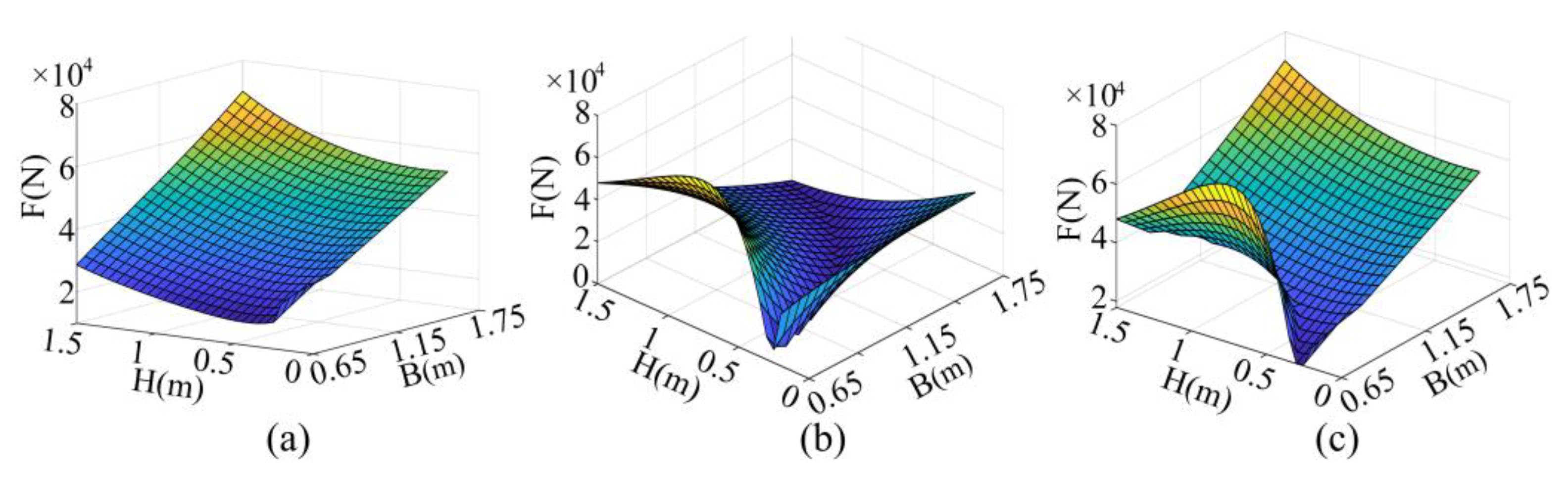
2.2.3. Adaptive Attitude in Terms of Energy Consumption

The hydraulic driving force of the legs of the hexapod robot was calculated, with Legs 1, 3, and 5 serving as support legs. Based on the leg structure and the planned foot force trajectory, the position of the foot-end relative to the base joint and the magnitudes of the large and small leg drive forces were analyzed for a constant foot-end force; the results for Leg 5 are shown in Figure 5a,b. Because the hexapod robot leg is hydraulically driven, the driving force of the hydraulic system is determined by the maximum load, which is given by the force on the side with the higher force. The relationships between the hydraulic-system drive force F and the geometric parameters H₀ and B₀ are shown in Figure 5c. It was observed that when B₀ is greater than 0.65 m and less than 1.75 m, the hydraulic system driving force F changes uniformly; with an increase in H₀, it initially decreases and subsequently increases, and it gradually increases with an increase in B₀.

In this study, we analyzed the impact of the center-to-ground height H of the hexapod robot torso form, torso-pitch angle α, and roll angle β on the energy consumption during a four-legged support movement (Leg 1, Leg 2, Leg 4, and Leg 5) across different terrains. Three terrain scenarios (φ_x = 5°, φ_y =30°; φ_x = 10°, φ_y =20°; and φ_x = 10°, φ_y =10°) were investigated.

The results shown in Figure 6 indicate that when the pitch angle φ_y of the terrain is small, and the α and β values are close to the terrain slope, the robot consumes less energy during one gait cycle. As the terrain slope decreases, the torso of the robot becomes parallel to the incline, resulting in an increased side-swing cylinder force and a reduced force on the thigh and lower leg cylinders. However, the cylinder pressure remained high at the base junction because the thigh and leg cylinders primarily supported the weight of the robot. The output pressure of the hydraulic system depends on the maximum load, resulting in minimal energy consumption at this stage. As per the analysis in Figure 5, the force required to maintain system balance varies under different postures. When the torso stance was not parallel to the support surface, a difference was observed in C_zj3 between the endpoints of the feet of the support legs in the torso coordinate system, which exacerbated the uneven output force of the hydraulic cylinders of each support leg and increased the energy consumption of the hydraulic system. In contrast, when the terrain slope angle was large, the maximum output pressure of the hydraulic system depended on the output pressure of the lateral swing cylinders, resulting in an increase in the output pressure of the hydraulic system.

As the center-to-ground height of the torso form increased, the energy consumption initially decreased and then increased. This is because the maximum force of the hydraulic system decreased and then increased with the variations in height H. Moreover, as height H increased, the range of available torso-pitch and roll angles also increased, which were constrained by the torso safety zone size and drive hydraulic-cylinder position limits. When the terrain slope increased, the stability constraint became dominant, restricting the torso’s attitude and reducing the range of selectable attitudes.

Different levels of energy consumption were observed for different terrains and body postures. On a rough terrain, the individual support legs required unique footing points, and legs with higher posture forces experienced smaller foot-end force distributions to minimize the energy usage of the overall system. Therefore, we optimized the postures, with the objectives of reduced energy consumption and increased use of the torso’s kinematics, and selected the appropriate torso postures so that the hydraulic drive force would be as small as possible and the torso’s workspace would be as large as possible. The optimization method was to collect multiple sets of simulation data as samples and use them to train a BP neural network model. The input was the terrain angle formed by the supporting feet and the initial height of the body, and the output was the body posture angle with the lowest energy consumption.

3. Force–Position Adaptive Impedance Control of Legs

3.1. Attitude Adaptive Adjustment

Figure 7 presents the overall control diagram of this study, which primarily includes terrain perception, trajectory planning, and controller components. The environment perception component comprises the terrain perception discussed in Section 2.1, as well as the obstacle detection based on the vision module. Following this, corresponding trajectory planning is conducted according to the perceived environment, mainly including safety constraints, stability control, and energy-optimal posture adjustment, as discussed in Section 2.2. Lastly, tracking control is performed on the foot-end force and cylinder position based on the trajectory planning.

A force–position composite control was employed to maintain body-posture stability during motion. The control method for the leg is the integration of an outer-loop adaptive fuzzy impedance algorithm with an inner-loop position control. The impedance controller generates the position correction ΔX based on the difference ΔF between the contact force F and the desired force Fr, and the motion position X_r is subsequently adjusted with the position correction ΔX. This enables the six-legged robot to maintain its body posture on a complex terrain by tracking the force.

In this study, the inner-loop position control utilized a neural network controller. A neural network controller, which continuously learns through feedback errors, was selected as the position controller; it gradually assumes the dominance of the control behavior. The outputs of the neural network control are as follows:

$$u(t)=u_n\left(t\right)+u_f\left(t\right)$$

(19)

where u_f(t) is the output of the PD control and u_n(t) is the output of the neural network model.

In the early stages of control, the feedback controller plays a predominant role, with the untrained neural network controller continuously learning through feedback errors. This is a process of simultaneous control and learning, possessing the ability to adapt to changes in the object and the environment. In this study, a three-layer feed-forward network has been utilized as the controller. The input–output relationship of the controller can be described as:

$$u_n\left(t\right)=W_{OH}^T\left(t\right)f\left[W_{HI}^T{X}_I\left(t\right)+{\theta }_H\left(t\right)\right]$$

(20)

where $X_I=\left\{r,e\left(t\right),\dots ,e\left(t-m+1\right)\right\}$ is the input vector of the network where r is the reference input; et is the tracking error; $W_{OH}^T\left(t\right)$$W_{HI}^T(t)$ are the weight matrices from the output layer to the hidden layer and the hidden layer to the input layer of the neural network controller; and ${\theta }_H\left(t\right)$ is the input bias of the hidden layer unit. The learning rules of the network weights can be derived according to the feedback error learning method, as:

$$\frac{d{[w\left(t\right),\theta \left(t\right)]}^T}{d\left(t\right)}=\eta \left(t\right)|\frac{\partial u_n\left(t\right)}{\partial \pi \left(t\right)}{|}^{T}E\left[u_f\left(t\right)\right]$$

(21)

where $\eta \left(t\right)$ is the learning rate; to avoid oscillations in the system, the following adaptive adjustment of the learning rate is used:

$$\eta \left(t\right)=2^{\lambda }\eta (t-1)$$

(22)

$$\lambda =sign[\begin{array}{cc}\frac{\partial u_n}{\partial {[w\left(\mathrm{t}\right),\theta \left(\mathrm{t}\right)]}^T}& \frac{\partial u_n}{\partial \pi (t-1)}\end{array}]$$

(23)

When the output of the PD feedback controller is smaller than the set threshold, the learning of the neural network ends temporarily, and the neural network controller completely replaces the feedback controller, controlling the system.

3.2. Adaptive Impedance Control

The position-based impedance control model can be conceptualized as a virtual spring model. Mathematically, the impedance control model can be expressed as a function of the robot forces, as follows:

$$\Delta F=M_d\Delta \ddot{X}+B_d\Delta \dot{X}+K_d\Delta X$$

(24)

where M_d, B_d, and K_d are the target inertia, target damping, and target stiffness matrices of the impedance control model for the robot, respectively; ΔF = F_r − F, ΔX = X − X_r. F and F_r represent the actual and desired contact forces, respectively, and X and X_r represent the actual and desired positions, respectively. When the foot-end of the robot is in contact with the environment, the impedance outer-loop control generates a position compensation value. This value represents an integrated control object consisting of the terrain environment and the foot-end of the robot. The contact model between the foot-end and the terrain environment can be simplified as follows:

$$F=M_e(\ddot{X}-{\ddot{X}}_e)+B_e(\dot{X}-{\dot{X}}_e)+K_{en}(X-X_e)$$

(25)

where the stiffness matrix (M_e), damping matrix (B_e), and stiffness matrix of the environment (K_en) are fundamental parameters used to describe the interaction of a legged robot with its surrounding terrain. X and X_e indicate the terrain positions.

When the foot-end maintains stable contact with the terrain, the small acceleration and velocity terms in the equation do not significantly affect the foot-end force (F) and can therefore be disregarded.

To simplify the contact model between the foot-end and the terrain environment, this study proposes using a spring model that considers the environmental stiffness (K_e), which is equivalent to the leg stiffness (K_l) and terrain environment stiffness (K_en) in series.

$$F=K_e(X-X_e)$$

(26)

In this study, we focused on the force in the z-direction, and the following equations were obtained from Equation (25):

$$\left\{\begin{array}{c}\dot{x}=\frac{\dot{f}}{k_e}+\dot{x}\\ \ddot{x}=\frac{\ddot{f}}{k_e}+{\ddot{x}}_e\end{array}\right.$$

(27)

After substituting Equation (27) into Equation (24), the following equation is obtained:

$$m_d^z{\ddot{e}}_f+b_d^z{\dot{e}}_f+(k_d^z+k_e^z)e_f=m_d^z\ddot{q}+b_d^z\dot{q}+k_d^{z}q$$

(28)

where $q=f_r^z+k_e^z{x}_e-k_e^z{x}_r$ and owing to the uncertainty of the terrain location, an estimation of environmental position $\widehat{x}$_e is utilized. By setting the desired trajectory x_r = _e, $q=f_r^z+k_e^z\eta x_e$.

The error function of the force is obtained according to Equation (28):

$$E(s)=\frac{(m_d^z{s}^2+b_d^{z}s+k_d^z)q(s)}{m_d^z{s}^2+b_d^{z}s+k_d^z+k_e^z}$$

(29)

Subsequently, the error equation for the steady-state force is:

$$e_{ss}=\underset{s\to 0}{\lim }sE(s)=\underset{s\to 0}{\lim }\frac{s(m_d^z{s}^2+b_d^{z}s+k_d^z)q(s)}{m_d^z{s}^2+b_d^{z}s+k_d^z+k_e^z}$$

(30)

When f_r is a constant force, the steady-state force error is:

$$e_{ss}=\frac{k_d^z(f_r^z+k_e^z\eta x_e)}{k_d^z+k_e^z}$$

(31)

Equation (31) shows that to achieve zero steady-state force error in impedance control, either condition $k_d^z$ = 0 or $f_r^z$ = $k_e^z$ηx_e must be satisfied. However, for a hexapod robot navigating a complex environment, it is challenging to measure the exact equivalent environmental stiffness (k_e) and position (x_e), which makes it difficult to satisfy the condition $f_r^z$ = $k_e^z$ ηx_e in practice. The center-of-gravity of the hexapod robot changed as it walked, resulting in a time-varying force at the foot-end. When f_r is a time-varying force, the steady-state force error still exists, even if $k_d^z$ = 0 is set. To mitigate this error, this study proposes an adaptive compensation algorithm to enhance the foot-end tracking performance against time-varying expected forces in the face of environmental uncertainty. Specifically, an adaptive compensation term is introduced into the control scheme.

$$\mathsf{\Gamma }(t)=\mathsf{\Gamma }(t-k)+\varsigma (f_r^z(t-k)-f^z(t-k))=\mathsf{\Gamma }(t-k)+\varsigma e_f^z(t-k)$$

(32)

where $\varsigma$ is the adaptive learning rate and k is the sampling period of the controller.

Assuming $k_d^z$ = 0 and incorporating the adaptive compensation term, the impedance model can be reformulated as follows:

$$m_d^z(\ddot{x}(t)-{\ddot{x}}_r(t))+b_d^z(\dot{x}(t)-{\dot{x}}_r(t))=e_f^z(t)+\mathsf{\Gamma }(t)$$

(33)

The steady-state force error equation can be re-derived as follows:

$$m_d^z{\ddot{e}}_f^z(t)+b_d^z{\dot{e}}_f^z(t)+k_e^z{e}_f^z(t)+k_e^z\mathsf{\Gamma }(t)=m_d^z\ddot{q}(t)+b_d^z\dot{q}(t)$$

(34)

Expanding the $\mathsf{\Gamma }(t)$, the first term of the expansion is set to zero, after which the expansion is applied to Equations (33) and (34).

$$m_d^z{\ddot{e}}_f^z(t)+b_d^z{\dot{e}}_f^z(t)+k_e^z{e}_f^z(t)+\varsigma k_e^z(e_f^z(t-(n+1)k)+\cdots +e_f^z(t-k))=m_d^z\ddot{q}(t)+b_d^z\dot{q}(t)$$

(35)

This equation can be transformed using Laplace to obtain the transfer function for the steady-state force error.

$$e_f(s)=\frac{m_d^z{s}^2+b_d^{z}s}{m_d^z{s}^2+b_d^{z}s+k_e^z+\varsigma k_e^z(e^{-(n+1)ks}+\cdots +e^{ks})}q(s)$$

(36)

The stability condition of the system can be determined using the Rouse stability criterion.

$$0<\varsigma <\frac{k{b}_d^z}{m_d^z+k{b}_d^z}$$

(37)

By substituting the constant force expectation and variable expectation force into the steady-state force error function as input signals, the corresponding table for the steady-state force error can be obtained, as shown in

Table 2. Steady-state error table for force tracking.

	fr = A	fr = Bt2	fr = ct2
IC	$k_{d}A/(k_e+k_d)$	∞	∞
KdZ = 0	0	$b_{d}B/k_e$	∞
AD	0	0	$m_{d}c/\sigma k_e$

. The proposed adaptive strategy enables force tracking to achieve convergence and eliminate steady-state errors.

Figure 8 depicts the joint simulation system constructed using MATLAB/Simulink and Adams to analyze the influence of m_d, b_d, and k_e on the control performance of the system. Figure 8c shows that as the target impedance inertia parameter m_d decreases, the response speed increases, while the regulation time and overshoot decrease. However, when the overshoot approaches a zero value, m_d decreases again, leading to a decrease in the response speed and an increase in the time required to reach a steady state. Figure 8b indicates that increasing b_d results in a decrease in the response speed and regulation time, whereas the absence of an overshoot leads to a decline in the response speed. However, when an overshoot is absent, increasing b_d leads to a decrease in the response speed. Figure 8a reveals that changes in the environmental stiffness parameters result in significant variations in the force-tracking performance. Therefore, we proposed a real-time self-adaptive fuzzy algorithm to adjust the impedance model parameters based on the error information determined between the expected and actual contact forces. This approach enhances the force-tracking performance of the impedance controller under different environmental parameters, thereby improving the adaptability of a six-legged robot to its surroundings.

The primary challenge in creating an impedance control system involves the selection of appropriate impedance control parameters to improve adaptability to varying environments. Therefore, we proposed a real-time self-adaptive fuzzy algorithm [29] to adjust the impedance model parameters based on the error information determined between the expected and actual contact forces.

The fuzzy control rules for the proposed method are as follows. When the error and error-change rate between the desired force at the foot-end and the contact force are significant, the target damping parameter should be small to enhance the system response. Conversely, when the error and error change rate between the desired force at the foot-end and contact force are negligible, the target damping parameter should be large to minimize the overshoot of the system and suppress its oscillation. Because the target inertia parameter md is sensitive to the dynamic response, and the effects of md and b_d on the control system are relatively similar, we adjusted the target damping parameter b_d to reduce the complexity of the control system. The input of the fuzzy controller is the error E_f between the expected force f_r at the foot-end and the contact force F, and the rate of change Ec_f of the force error is calculated using Equation (38). The output of the fuzzy controller is an increment in the target damping parameter of the impedance controller.

$$\left\{\begin{array}{l}{E}_f=(F_r-F)\\ E{c}_f=\frac{E_f}{\kappa }\end{array}\right.$$

(38)

where $\kappa$ represents the sampling period.

The theoretical domain of the input and output quantities of the fuzzy controller is considered as [−1, 1], and the corresponding normalization coefficients transform the ranges of the input and output quantities into the theoretical domain interval. The output of the fuzzy controller is an increment in the target damping parameter of the impedance controller.

$$\left\{\begin{array}{l}{\tilde{E}}_f=\frac{2}{E_{f\max }-E_{f\min }}\cdot (E_f-\frac{E_{f\max }+E_{f\min }}{2})\\ \tilde{E}{c}_f=\frac{2}{E{c}_{f\max }-E{c}_{f\min }}\cdot (E{c}_f-\frac{E{c}_{f\max }+E{c}_{f\min }}{2})\\ \Delta b=\frac{\Delta \tilde{b}(\Delta b_{\max }-\Delta b_{\min })}{2}+\frac{\Delta b_{\max }+\Delta b_{\min }}{2})\end{array}\right.$$

(39)

where E_fmax, E_fmin, Ec_fmax, Ec_fmin, Δb_max, and Δb_min are the maximum and minimum values of E_f, Ec_f and Δb, respectively.

The fuzzy inference process, as shown in Figure 9, involves dividing the various input and output quantities of the fuzzy controller into seven fuzzy levels [NB, NM, NS, ZE, PS, PM, PB], which increase in order from NB to PB. The Gaussian-type subordination function was selected as the subordination function. The fuzzy control rules and image of the affiliation function for the target damping parameter adjustment were established according to the principle of target damping parameter adjustment. The parallel method was used for fuzzy inference, and the center-of-gravity method was used for defuzzification. The increment of the normalized target damping parameter $\Delta \tilde{b}$ was obtained.

3.3. Force Tracking Experiment

To validate the ability of the force-tracking algorithm to operate on real robots on different terrains, this study conducted experimental investigations on terrain obstacles of varying environmental stiffness. The torso height of the robot was set to 0.4 m above the ground, the gait period was 2 s. The experimental setup involved using the five legs of the hexapod robot as supports while moving the remainder leg within three different terrain environments: hard ground, soft foam ground, and soil. The movements included swing, contact, and foot force tracking. The inertia parameter was set to md = 100 kg, and the input quantity ranges of the fuzzy controllers E_f and Ec_f were [−5000, −5000] and [−1000, 1000], respectively. The initial value of the damping parameter was bd = 2000 N/(m/s), and the output damping parameter adjustment range was [−5000, 5000]. Figure 10 illustrates the experimental results of the robot on different terrains by comparing different force-tracking algorithms.

The force-tracking curves in different terrain environments displayed different responses, as shown by the experimental results. In hard-terrain environments, where the landing impact was greater, both foot force tracking algorithms exhibited faster responses, as shown in Figure 10e,f. The adaptive compensation algorithm (AD) for force tracking showed a response process similar to that of the traditional impedance control (IC), owing to the large equivalent terrain stiffness of the hard terrain, which resulted in a small steady-state error. On the soft-foam terrain (Figure 10c,d), where the impact force when the foot-end falls to the ground is low, the IC algorithm tracking of the desired acceleration force showed a state of nonconvergence of the force steady-state error. However, as the leg was compressed, the equivalent environmental stiffness gradually increased, and the steady-state error decreased. The AD algorithm improved the response speed and exhibited a relatively small steady-state force error. As shown in Figure 10a,b, the impact force on the foot-end hitting the ground is negligible on the soil. Owing to the lower equivalent stiffness of the soil terrain environment, the response of the IC algorithm becomes slower, and the steady-state force error in force tracking increases. The steady-state error decreases as the soil is compressed, and the equivalent environmental stiffness increases.

The AD algorithm tracks the slope expectation force with a faster response rate and convergence in the steady-state error of force for tracking the acceleration expectation force. The performance of the force-tracking effect is better than that of the IC, which not only improves the response speed, but also results in a relatively small force–steady-state error. However, the adaptive fuzzy (AF) algorithm demonstrated improved performance in force tracking, resulting in a better response speed and reduced force overshoot. Overall, the introduction of the response process increased the amount of overshoot in the system response compared with that without the AD. The introduction of the AF algorithm resulted in relatively better tracking of slope forces at the foot-end of the leg.

4. Experimental Studies and Discussion

The experimental platform utilized for the study of the six-legged robot discussed in this study is depicted in Figure 11. The hexapod had a total mass of 3.55 metric tons, with an electrohydraulic servo mechanism based on hydraulic propulsion. Once the desired trajectory was established, the corresponding current value was input to the servo valve to regulate the movement of the hydraulic cylinder associated with the valve, which was equipped with a built-in displacement sensor to provide feedback regarding its position. A hydraulic pump supplied by Danfoss offered a maximum output pressure of 31 MPa.

The robot features a force sensor and an attitude and heading reference system to enable monitoring of the vehicle’s status. The distributed visual perception system was set up using the Nvidia Jetson Nano processor and the PyTorch framework. The YOLOv5 algorithm [30] was used as a neural network algorithm. The categories of obstacles were set as tree trunks, people, cars, and boulder. The samples of relevant detection results are shown in Figure 10, and the information of obstacles was transmitted to the motion controller through serial communication. Following calibration, the error between the obstacle coordinates obtained from the vision module and the actual coordinates was found to be less than 8 mm. This level of precision enables the supply of obstacle information for the obstacle-avoidance strategy outlined in Section 2.2.1. The control approach involves a hardware-in-the-loop system that utilizes an embedded control host powered by the VxWorks operating system with a control cycle of 1 ms and real-time data transmission facilitated through UDP communication to the host computer. The multi-sensor data type and driver configurations were established on the PCI board, and the program’s real-time simulation model and driver were developed using MATLAB/Simulink. The simulation program was coded using Microsoft Visual Studio. The structure of the neural model in this experiment was set as $3\times 8\times 1$, the initial weights of the neural network were randomly selected within [−0.1, 0.1], the learning rate was set as 0.07, and the value range of the neuron selection sigmoid activation function was [−1, 1]. The parameters of the adaptive fuzzy impedance were set to be the same as the experimental parameters in Section 3.3.

First, the effect of the force–position composite control algorithm on the posture of the torso during motion was compared. The experimental scenario is shown in Figure 12. The full cycle consisted of three steps, with two legs for swing in each step and the remaining four legs for support. This gait style is more suitable for complex terrain, because it has higher stability than three-legged support. The base junction foot-end phase began at an initial height of −0.4 m, and the motion step length was 0.8 m. Each step took 3 s, with a 0.3 m lift in the z-direction when swinging. The motion trajectory of the robot used a low-impact foot-end trajectory method that facilitated the initial position and velocity constraints by employing acceleration as a sinusoidal function.

The trajectory of the leg on one side of the hexapod robot during position-based control relative to its initial stance in the forward Y-direction and vertical Z-direction is shown in Figure 13a. Each side of the robot has two support-legs and one swing-leg involved in each gait cycle, and the force on each leg is shown in Figure 13b, where the right front (RF) leg and right middle (RM) leg step on the obstacle at 2.73 s and 5.45 s, respectively. The larger force generated when the obstacle is stepped on also affects the forces on the other legs, which has a greater impact on the torso stance of the body. During the support process, owing to the uncertainty of the terrain, the position of the center-of-mass changes accordingly at different slopes, leading to a large deviation in the force of each leg from the expected force, when the posture of the robot torso is influenced by the environment. The robot’s torso posture is shown in Figure 13c, and due to the irregular terrain of the landing point, the robot’s roll and pitch angles have undergone significant changes. Figure 13d,e show the z-direction coordinates of the legs in the force–position control situation and the forces acting on the legs; it can be seen that when the obstacles are encountered during the swing phase at 2.65 s and 5.68 s, the sensor detects the changes in force and avoids the obstacles by adjusting the displacement in the z-direction, which is adjusted to avoid the movement of the entire vehicle. In the support phase, the change in the displacement in the z-direction is adjusted according to the change in the support force, thus ensuring that the desired force of the leg to the torso support agrees better, and that the foot-end force can fluctuate around the desired force to achieve dynamic equilibrium. The posture of the robot’s trunk is shown in Figure 13f, and it can be seen that the robot can maintain stability of the trunk after a brief adjustment during phase switching. This indicates that the control method proposed in this article can enable the robot to maintain the target attitude while moving in complex terrain.

To validate the posture optimization method adapted for various terrains, experiments were conducted using two types of terrains: the hillside, with a pitch angle of 10°, and asphalt pavements which had a pitch angle of 14°, as shown in Figure 14. Experiments were conducted with the hexapod robot walking on a slope at different trunk center-of-mass heights (H) and trunk pitch angles (φ_y). The robot’s total energy consumption for each stride was determined through the pressure and flow of the hydraulic system. The system’s working pressure was obtained through a pressure sensor, and the working flow was calculated based on the cylinder displacement. As shown in Figure 15, it can be observed that under two slope conditions, the energy consumption of the hexapod robot with the growth of H exhibits a trend of initially decreasing and then increasing. Moreover, as the trunk pitch angle increases, the energy consumption gradually decreases. At a terrain pitch angle of φ_y = 10° and a trunk center-of-mass height of H = 400 mm, the minimum energy consumption occurred when the trunk pitch angle was at 10°. The theoretically calculated result was 34.2 kJ, while the experimental result was 36.1 kJ. When the estimated slope was at a pitch angle of φ_y = 14°, the minimum energy consumption of the hexapod robot occurred at a trunk center-of-mass height of H = 400 mm and a trunk pitch angle of 14°. The theoretical result was 33.1 kJ, and the experimental result was 35.0 kJ. The actual energy consumption of the robot hydraulic system in each step is shown in

Table 3. Table of actual energy consumption.

	Pitch Angle	H = 200 mm	H = 300 mm	H = 400 mm	H = 500 mm
φy = 10°	0°	-	-	49.7	54.2
	2°	-	46.4	45.9	49.8
	4°	43.1	44.0	43.1	46.7
	6°	40.3	40.6	40.6	43.2
	8°	38.7	37.9	37.5	40.8
	10°	36.3	35.9	36.1	40.0
φy = 14°	2°	-	-	-	55.2
	4°	-	-	50.1	50.8
	6°	-	48.6	46.9	46.6
	8°	45.7	45.7	43.4	43.2
	10°	42.7	41.8	39.6	39.9
	12°	39.5	39.2	37.0	38.0
	14°	37.9	36.5	35.0	36.6

. These results indicate a certain discrepancy between the theoretically calculated energy consumption and the actual values. This discrepancy is due to additional energy consumption caused by pressure shocks and position errors during the actual motion process. However, the trend of energy consumption changes with posture being observed in actual walking is consistent with the theoretically calculated energy consumption, thereby validating the effectiveness of the posture optimization strategy proposed in this study.

To validate the performance of the proposed self-adaptive fuzzy impedance control method for actual robot motion, we conducted a comparative analysis of the proposed method with the impedance control method (ICM) used in the previous reference [15]. As shown in Figure 14, the robot fell into the hillside pavement while moving, indicating that the hillside pavement was less stiff than the rigid asphalt pavement Because terrain uncertainty has a significant impact on the comparative study results, a transition phase was added in the phase-switching process by introducing a six-legged co-supported gait before the switching phases, and a constant force was set as the expected force of the support leg during this phase.

The experimental results are shown in Figure 16. The right rear (RR) leg of the robot was the focus of this study, and a three-step motion was used. The movements proceeded as follows: 1–2 s of the swing phase, where the expected force is zero; 2–2.5 s of the transition phase, where the RR leg serves as the support for the next phase of the gait, and the expected force is constant at 6000 N; and 2.5–5 s of the support phase, where the expected force is obtained through trajectory planning and foot force distribution algorithms, resulting in a variable force at variable acceleration. As shown in Figure 16a, both control algorithms exhibit faster responses on hard terrain. The steady-state error in the force did not differ significantly. Figure 16b,c shows the displacement compensation of the two control algorithms and the pitch angle of the robot body in the z-direction at this stage. The tilt angle of the robot body is smaller during the switching phase, and the control effects of the two algorithms are approximately the same.

The performance of legged robots is significantly affected on hillside terrain, where the ground stiffness is low. The experimental results depicted in Figure 16d show that, during the transition phase, the ICM is more sensitive to the environment, causing a slower response while tracking the constant force and resulting in force-tracking errors of constant-force tracking during the gait time. In the support phase, the traditional impedance method establishes the target support force in 0.43 s, while the AF control algorithm proposed in this study establishes the target support force in 0.16 s. Both control algorithms exhibit improved desired force-tracking effects, because the robot compressed the soil during the motion, owing to self-weight. This improved the terrain stiffness, particularly by adding a transition phase, thereby reducing the steady-state error. As shown in Figure 16f, in the low-stiffness environments and during phase switching, the maximum tilt angle of the body is 0.37°, whereas the maximum tilt angle of the impedance control is 0.88°. Because of the small compensation amount of the ICM during phase switching, the body experienced a brief tilt instability caused by the low stiffness of the ground, thereby failing to establish support in time.

The rugged terrain and asphalt pavement are considered as soft and hard terrain, respectively, and the experimental results are shown in

Table 4. Table of force-tracking performance.

		Maximum Error of Pitch Angle	Steady-State Time
Hard terrain	ICM	0.25°	0.11 s
	AF	0.24°	0.15 s
Soft terrain	ICM	0.88°	0.43 s
	AF	0.37°	0.16 s

. The results demonstrated that the AF algorithm exhibits improved performance in force tracking when the terrain environment is relatively “soft”, whereas the performance improvement of the AF algorithm is less significant when the terrain environment is “hard”. Moreover, it was observed that the convergence process of the ICM for force tracking becomes slower as the terrain environment becomes relatively “soft”, whereas the AF algorithm demonstrates better performance in improving force tracking in such environments and exhibits certain adaptability to the terrain. However, compared with the single-leg study, the overall tracking performance of the robot experiment decreased and fluctuated owing to the influences of the position-control accuracy and rigid-flexible coupling characteristics of the heavy-duty robot itself, as well as force-tracking errors caused by uncertainties.

5. Conclusions

In this paper, we propose a motion strategy for agricultural transportation robots operating on complex terrains. The premise of the motion strategy looks to torso safety and stability constraints based on the terrain estimation of the support surface, and a visual recognition system to ensure the safe passage of the robot on different terrains. Moreover, force analysis of the hydraulic leg drive was conducted to establish the correspondence between the driving force and the motion posture. It can be concluded that adjusting the robot’s posture can reduce the energy consumption of robot movements. A control method combining force and position was subsequently proposed, maintaining the target posture of the robot’s torso through force tracking. To address the problem of tracking time-varying forces in uncertain environments, an adaptive-fuzzy impedance algorithm was developed to eliminate steady-state errors. The proposed control strategy was validated by building a real-time simulation system for a heavy-duty six-legged robot and comparing it with an existing model. Experimental and simulation results showed that the robot maintained the stability of its locomotor posture by tracking the forces on each leg, and the proposed control strategy achieved convergence and shorter response times on various terrains. The proposed control method is able to reduce the adjustment time of the system by 58% and the deflection error of the structure by 62.8% when the stiffness of the external environment is low.

Several issues remain to be resolved before the advent of the widespread use of multi-legged hydraulic robots. These include the fact that hydraulic drive units in swing and support states require different driving forces, but the solution provided by a single-pump hydraulic systems fails to satisfy the differing requirements of multiple legs, leading to energy loss. Another issue is that the flexible deformation of the legs in large-sized, heavy-load robots makes force tracking difficult for the system. Therefore, in the near future, we plan to modify the structure of our hydraulic system and optimize our control algorithms to overcome these challenges.

References

1. Yuan, J.; Ji, W.; Feng, Q. Robots and Autonomous Machines for Sustainable Agriculture Production. Agriculture 2023, 13, 1340. [Google Scholar] [CrossRef]
2. Tiozzo Fasiolo, D.; Scalera, L.; Maset, E.; Gasparetto, A. Towards Autonomous Mapping in Agriculture: A Review of Supportive Technologies for Ground Robotics. Robot. Auton. Syst. 2023, 169, 104514. [Google Scholar] [CrossRef]
3. Gai, J.; Xiang, L.; Tang, L. Using a Depth Camera for Crop Row Detection and Mapping for Under-Canopy Navigation of Agricultural Robotic Vehicle. Comput. Electron. Agric. 2021, 188, 106301. [Google Scholar] [CrossRef]
4. Vrochidou, E.; Tsakalidou, V.N.; Kalathas, I.; Gkrimpizis, T.; Pachidis, T.; Kaburlasos, V.G. An Overview of End Effectors in Agricultural Robotic Harvesting Systems. Agriculture 2022, 12, 1240. [Google Scholar] [CrossRef]
5. Ferreira, J.; Moreira, A.P.; Silva, M.; Santos, F. A Survey on Localization, Mapping, and Trajectory Planning for Quadruped Robots in Vineyards. In Proceedings of the 2022 IEEE International Conference on Autonomous Robot Systems and Competitions (ICARSC), Santa Maria da Feira, Portugal, 29–30 April 2022. [Google Scholar]
6. Song, X.; Zhang, X.; Meng, X.; Chen, C.; Huang, D. Gait Optimization of Step Climbing for a Hexapod Robot. J. Field Robot. 2021, 39, 55–68. [Google Scholar] [CrossRef]
7. Lee, W.-J.; Orin, D.E. The Kinematics of Motion Planning for Multilegged Vehicles over Uneven Terrain. IEEE J. Robot. Autom. 1988, 4, 204–212. [Google Scholar] [CrossRef]
8. Xu, K.; Lu, Y.; Shi, L.; Li, J.; Wang, S.; Lei, T. Whole-Body Stability Control with High Contact Redundancy for Wheel-Legged Hexapod Robot Driving over Rough Terrain. Mech. Mach. Theory 2023, 181, 105199. [Google Scholar] [CrossRef]
9. Choi, S.; Ji, G.; Park, J.; Kim, H.; Mun, J.; Lee, J.H.; Hwangbo, J. Learning Quadrupedal Locomotion on Deformable Terrain. Sci. Robot. 2023, 8, eade2256. [Google Scholar] [CrossRef] [PubMed]
10. Kalakrishnan, M.; Buchli, J.; Pastor, P.; Mistry, M.; Schaal, S. Learning, Planning, and Control for Quadruped Locomotion over Challenging Terrain. Int. J. Robot. Res. 2010, 30, 236–258. [Google Scholar] [CrossRef]
11. Grzelczyk, D.; Stanczyk, B.; Awrejcewicz, J. Kinematics, Dynamics and Power Consumption Analysis of the Hexapod Robot During Walking with Tripod Gait. Int. J. Struct. Stab. Dyn. 2017, 17, 1740010. [Google Scholar] [CrossRef]
12. Ott, C.; Mukherjee, R.; Nakamura, Y. Unified Impedance and Admittance Control. In Proceedings of the 2010 IEEE International Conference on Robotics and Automation, Anchorage, AK, USA, 3–7 May 2010. [Google Scholar]
13. Zhu, Q.; Huang, D.; Yu, B.; Ba, K.; Kong, X.; Wang, S. An Improved Method Combined SMC and MLESO for Impedance Control of Legged Robots’ Electro-Hydraulic Servo System. ISA Trans. 2022, 130, 598–609. [Google Scholar] [CrossRef]
14. Zhu, Q.; Zhang, J.; Li, X.; Zong, H.; Yu, B.; Ba, K.; Kong, X. An Adaptive Composite Control for a Hydraulic Actuator Impedance System of Legged Robots. Mechatronics 2023, 91, 102951. [Google Scholar] [CrossRef]
15. Wang, S.; Chen, Z.; Li, J.; Wang, J.; Li, J.; Zhao, J. Flexible Motion Framework of the Six Wheel-Legged Robot: Experimental Results. IEEE/ASME Trans. Mechatron. 2022, 27, 2246–2257. [Google Scholar] [CrossRef]
16. Kronander, K.; Billard, A. Stability Considerations for Variable Impedance Control. IEEE Trans. Robot. 2016, 32, 1298–1305. [Google Scholar] [CrossRef]
17. Roveda, L.; Iannacci, N.; Vicentini, F.; Pedrocchi, N.; Braghin, F.; Tosatti, L.M. Optimal Impedance Force-Tracking Control Design With Impact Formulation for Interaction Tasks. IEEE Robot. Autom. Lett. 2016, 1, 130–136. [Google Scholar] [CrossRef]
18. Deng, Z.; Jin, H.; Hu, Y.; He, Y.; Zhang, P.; Tian, W.; Zhang, J. Fuzzy Force Control and State Detection in Vertebral Lamina Milling. Mechatronics 2016, 35, 1–10. [Google Scholar] [CrossRef]
19. Yang, J.; Sun, T.; Yang, H. Spatial Hybrid Adaptive Impedance Learning Control for Robots in Repetitive Interactive Tasks. ISA Trans. 2023, 138, 151–159. [Google Scholar] [CrossRef]
20. Wang, W.; Li, Q.; Lu, C.; Gu, J.; Li, A.; Li, Y.; Huo, Q.; Chu, H.; Zhu, M. Impedance Estimation for Robot Contact with Uncalibrated Environments. Mech. Syst. Signal Process. 2021, 159, 107819. [Google Scholar] [CrossRef]
21. Huang, B.; Ye, Z.; Li, Z.; Yuan, W.; Yang, C. Admittance Control of a Robotic Exoskeleton for Physical Human Robot Interaction. In Proceedings of the 2017 2nd International Conference on Advanced Robotics and Mechatronics (ICARMT), Ai’an, China, 27–31 August 2017. [Google Scholar]
22. Yang, C.; Zeng, C.; Fang, C.; He, W.; Li, Z. A DMPs-Based Framework for Robot Learning and Generalization of Humanlike Variable Impedance Skills. IEEE/ASME Trans. Mechatron. 2018, 23, 1193–1203. [Google Scholar] [CrossRef]
23. Zeng, C.; Yang, C.; Cheng, H.; Li, Y.; Dai, S.-L. Simultaneously Encoding Movement and sEMG-Based Stiffness for Robotic Skill Learning. IEEE Trans. Ind. Inform. 2021, 17, 1244–1252. [Google Scholar] [CrossRef]
24. Zhang, T.; Liang, X.; Zou, Y. Robot Peg-in-Hole Assembly Based on Contact Force Estimation Compensated by Convolutional Neural Network. Control. Eng. Pract. 2022, 120, 105012. [Google Scholar] [CrossRef]
25. Modares, H.; Ranatunga, I.; Lewis, F.L.; Popa, D.O. Optimized Assistive Human–Robot Interaction Using Reinforcement Learning. IEEE Trans. Cybern. 2016, 46, 655–667. [Google Scholar] [CrossRef]
26. Yang, Y.; Wu, X.; Song, B.; Li, Z. Whole-Body Fuzzy Based Impedance Control of a Humanoid Wheeled Robot. IEEE Robot. Autom. Lett. 2022, 7, 4909–4916. [Google Scholar] [CrossRef]
27. Homchanthanakul, J.; Manoonpong, P. Continuous Online Adaptation of Bioinspired Adaptive Neuroendocrine Control for Autonomous Walking Robots. IEEE Trans. Neural Netw. Learn. Syst. 2022, 33, 1833–1845. [Google Scholar] [CrossRef]
28. Li, Z.; Ge, Q.; Ye, W.; Yuan, P. Dynamic Balance Optimization and Control of Quadruped Robot Systems With Flexible Joints. IEEE Trans. Syst. Man Cybern. Syst. 2016, 46, 1338–1351. [Google Scholar] [CrossRef]
29. Ferraz, R.S.C.; Mello, T.P.; Borges Filho, M.N.; Borges, R.F.O.; Magalhães Filho, S.C.; Scheid, C.M.; Meleiro, L.A.C.; Calçada, L.A. An Experimental and Theoretical Approach on Real-Time Control and Monitoring of the Apparent Viscosity by Fuzzy-Based Control. J. Pet. Sci. Eng. 2022, 217, 110896. [Google Scholar] [CrossRef]
30. Lu, A.; Ma, L.; Cui, H.; Liu, J.; Ma, Q. Instance Segmentation of Lotus Pods and Stalks in Unstructured Planting Environment Based on Improved YOLOv5. Agriculture 2023, 13, 1568. [Google Scholar] [CrossRef]
Figure 1. Structure of hexapod robot.
Agriculture 13 02131 g001
Figure 2. Flowchart of terrain awareness strategy.
Agriculture 13 02131 g002
Figure 3. Diagram of reference coordinate system.
Agriculture 13 02131 g003
Figure 4. (a) Yaw angle adjustment of the torso; (b) sketch of the NESM solution.
Agriculture 13 02131 g004
Figure 5. Analysis of hydraulic drive forces for the legs. (a) Thigh cylinder. (b) Shin cylinder. (c) Hydraulic driven force.
Agriculture 13 02131 g005
Figure 6. Relationship between posture and energy consumption on different terrains.
Agriculture 13 02131 g006
Figure 7. Diagram of motion strategy for heavy-duty hexapod robot.
Agriculture 13 02131 g007
Figure 8. Analysis of the influence of impedance parameters.
Agriculture 13 02131 g008
Figure 9. Flowchart of the fuzzy-logic control.
Agriculture 13 02131 g009
Figure 10. Performance of force tracking for different environmental stiffnesses. (a) Slope force tracking in soft soil terrain. (b) Slope force tracking in soft foam terrain. (c) Slope force tracking in hard terrain. (d) Acceleration force tracking in soft soil terrain. (e) Acceleration force tracking in soft foam terrain. (f) Acceleration force tracking in hard terrain.
Agriculture 13 02131 g010
Figure 11. Experimental platform for heavy-duty transport robot.
Agriculture 13 02131 g011
Figure 12. The motion process of the hexapod robot in complex terrain.
Agriculture 13 02131 g012
Figure 13. Comparison of motion states for mixed force–position control. (a) End-of-foot tracking by position control. (b) Force at the end of the foot controlled by position (c) Angle of the trunk controlled by position. (d) End-of-foot tracking via position-force control. (e) End-of-foot force tracking via position-force control. (f) Angle of the torso via position-force control.
Agriculture 13 02131 g013
Figure 14. Experimental scenarios in different stiffness environments.
Agriculture 13 02131 g014
Figure 15. Performance comparison of different force-tracking algorithms.
Agriculture 13 02131 g015
Figure 16. Performance comparison of different force tracking algorithms. (a) force tracking in hard terrain, (b) position compensation in hard terrain, (c) torso angle in hard terrain, (d) force tracking in soft terrain, (e) position compensation in soft terrain, (f) torso angle in soft terrain.
Agriculture 13 02131 g016