Article

Predicting Sugarcane Yield via the Use of an Improved Least Squares Support Vector Machine and Water Cycle Optimization Model

State Key Laboratory for the Protection and Utilization of Subtropical Agricultural Biological Resources, College of Mechanical Engineering, Guangxi University, Nanning 530004, China
*
Author to whom correspondence should be addressed.
Agriculture 2023, 13(11), 2115; https://doi.org/10.3390/agriculture13112115
Submission received: 6 October 2023 / Revised: 2 November 2023 / Accepted: 6 November 2023 / Published: 8 November 2023
(This article belongs to the Special Issue Application of Machine Learning and Data Analysis in Agriculture)

Abstract

:
As a raw material for sugar, ethanol, and energy, sugarcane plays an important role in China’s strategic material reserves, economic development, and energy production. To guarantee the sustainable growth of the sugarcane industry and boost sustainable energy reserves, it is imperative to forecast the yield in the primary sugarcane production regions. However, due to environmental differences caused by regional differences and changeable climate, the accuracy of traditional models is generally low. In this study, we counted the environmental information and yield of the main sugarcane-producing areas in the past 15 years, adopted the LSSVM algorithm to construct the environmental information and sugarcane yield model, and combined it with WCA to optimize the parameters of LSSVM. To verify the validity of the proposed model, WCA-LSSVM is applied to two instances based on temporal differences and geographical differences and compared with other models. The results show that the accuracy of the WCA-LSSVM model is much better than that of other yield prediction models. The RMSE of the two instances are 5.385 ton/ha and 5.032 ton/ha, respectively, accounting for 7.65% and 6.92% of the average yield. And the other evaluation indicators MAE, R2, MAPE, and SMAPE are also ahead of the other models to varying degrees. We also conducted a sensitivity analysis of environmental variables at different growth stages of sugarcane and found that in addition to the main influencing factors (temperature and precipitation), soil humidity at different depths had a significant impact on crop yield. In conclusion, this study presents a highly precise model for predicting sugarcane yield, a useful tool for planning sugarcane production, enhancing yield, and advancing the field of agricultural production prediction.

1. Introduction

Sugarcane is a perennial crop of the grass family, mainly found in the tropics, and is the main raw material for sugar production [1], contributing to more than 90% of sugar production in China [2]. Simultaneously, sugarcane bagasse has emerged as a promising and versatile composite material component, attracting widespread attention for its potential as a viable alternative energy source due to its natural, biodegradable properties and chemical composition [3]. This bio-residue is currently considered by many researchers as a low-carbon alternative to fossil fuels [4] and is considered to be the most promising material for low-cost sustainable biofuels (e.g., ethanol) and power generation [5]. The importance of the sugarcane industry is not limited to food, ethanol, or electricity production. Sugarcane and its residues can also produce many value-added products, including various biofuels, biomaterials, biochemicals, and bioenergy, obtained through biological refining. This has promoted the development of sustainable economy. China ranks third in global sugarcane production behind Brazil and India [6]. Among them, the southern provinces of Guangxi, Hainan, Guangdong, and Yunnan are the main producing regions, which have similar climatic characteristics: strong solar radiation, abundant rainfall, and high average temperatures. The main production area can reach 1.5 million hectares, and sugarcane yields account for more than 95% of the country. In Guangxi, for example, between 2012 and 2013, the sugar industry’s gross domestic product (GDP) was 43.58 billion yuan, accounting for 3.33 percent of Guangxi’s total GDP, and farmers’ income from sugarcane reached 32.26 billion yuan. In addition, the sugar industry also provides many opportunities for other industries such as transportation, marketing, and employment, leading to overall socio-economic development. To guarantee high yields of sugarcane and foster the advancement of sustainable economics, it is imperative to forecast the sugarcane yield.
Yield forecasting is a key component used in the crop production planning process for setting goals, evaluating alternatives, and assigning management plans. Yield prediction relies on modern techniques, which can improve the sustainability of the industry and explore the influence of various variables on yield for agricultural production. Given the long growth cycle of sugarcane, if the available information that can be used to generate better yield predictions increases, there are more opportunities to modify the predictions and optimize growth planning for sugarcane yield. However, yield has a high variance and is difficult to predict in agricultural research [7]. This is because sugarcane production is affected by several factors, including precipitation, temperature, water, nutrients, natural disasters, and field management [8]. Therefore, many researchers are committed to developing a crop growth model that can be coupled with multiple factors to predict sugarcane yield. For example, the DSSAT-CANEGRO model based on carbon balance and water balance was proposed and improved [9], and then a software system, APSIM, was developed for agricultural systems research, which can be used for crop yield prediction. With the emergence of Artificial Intelligence, machine learning [10,11] has overcome the limitations of traditional methods and is capable of recognizing nonlinear patterns in large datasets; hence, it has been widely used for crop yield prediction. Preeti Saini et al. [12] validated models such as LSTM, GPR, and Holt-winter time series for the traditional prediction of sugarcane. The results showed that the LSTM model had the highest prediction accuracy with RMSE and MSE of 8.8 and 77.79. dos Santos Luciano A C et al. [13] calibrated three RF models using different predictors to predict sugarcane yield at harvest. The results showed that the optimal RF model had a root mean square error (RMSE) of 9.9 tons ha in yield prediction. Das A et al. [14] developed an opti-SAR sugarcane yield prediction model with an integrated machine learning algorithm. The results showed that the accuracy of the integrated model was better than that of the single-base model. And the accuracy of the prediction model was high 1–2 months before the sugarcane harvest. Ilyas Q M et al. [15] combined machine learning algorithms with remote sensing to predict yields of linseed, lentil, rice, sugarcane, and wheat, and found that the model outperformed individual classification methods in classifying crop types and had relatively low mean square error values for the returns.
However, in the traditional machine learning model, the sugarcane yield prediction considers too many single influencing factors, and the prediction accuracy is hardly satisfactory. On the one hand, regional differences lead to different environmental variables of sugarcane growth, which have a greater impact on the prediction accuracy of sugarcane yield models [16,17]. On the other hand, the decrease in the prediction accuracy of the crop growth model is a result of the overall change in climate due to temporal differences [18]. Summing up the above two factors, it is difficult to predict future yields based on environmental factors in different regions and historical environmental factors. Therefore, many scholars have combined climate prediction models for certain regions using crop growth models. Climate prediction models are used to simulate future climate changes in the region and attempt to approximate the real sugarcane yield under climate changes. At present, many researchers have applied machine learning algorithms to continuously improve and update climate prediction models [19,20,21], but improving yield prediction models is not ideal. This is attributed to the fact that fewer studies have been conducted on combining machine learning algorithms with climate prediction models to predict regional yields of sugarcane [22]. In addition, the accuracy of sugarcane-related models is generally low (RMSE from 19.7 to 20.0 ton/ha), which needs to be improved.
In order to improve the prediction accuracy of machine learning algorithms when combined with climate prediction models, it is necessary to find suitable methods to optimize them. The water cycle algorithm is an algorithm for scheduling and allocating tasks in the model. Its core idea is to reasonably arrange the execution order of tasks and resource allocation according to the priority of tasks and resource demand, in order to improve the performance of the model and resource utilization. The water cycle algorithm is able to realize the fusion exploration of meteorological data, soil data, terrain data, and other multivariate data, and at the same time, it can be highly compatible with machine learning algorithms and climate prediction models [23,24]. In summary, the water cycle algorithm has high potential in optimizing sugarcane yield prediction models.
Uncertainty is inevitable when using any individual machine learning model in isolation due to lack of comparison. Optimization can solve the problem of predictive accuracy of machine learning models, but not the uncertainty of individual model estimates. The objective of this study is to select three machine learning algorithms, such as BPNN, RF, and LSSVM. Based on the main sugarcane production areas in southern China, an environmental variable sugarcane yield prediction model is developed with environmental information during the sugarcane growth cycle. And the model is applied to two instances of time difference and regional difference to verify the validity and accuracy. In addition, to further improve the prediction accuracy, the algorithm parameters are optimized to achieve reliable yield prediction. And the effects of environmental variables on sugarcane yield during each growth cycle are analyzed. The research objectives include the following: (1) validating the feasibility of the WCA_LSSVM prediction model proposed in this paper in regional production potential simulation; (2) comparing the performance of sugarcane yield models in regional production potential simulation based on different machine learning algorithms; (3) selecting and evaluating the most critical regional environmental variables in machine learning-based sugarcane yield prediction models.
This study is organized as follows. In Section 2, the process of building the BPNN, RF, and LSSVM prediction models and the principle of the water cycle optimization method are introduced. Section 3 presents a comparison of the prediction results of the three machine learning models, as well as a comparison of the optimization results of the particle swarm optimization method and the water cycle optimization method. Section 4 summarizes the conclusions obtained from the comparative analysis of the prediction models and provides an outlook for future work.

2. Methodology

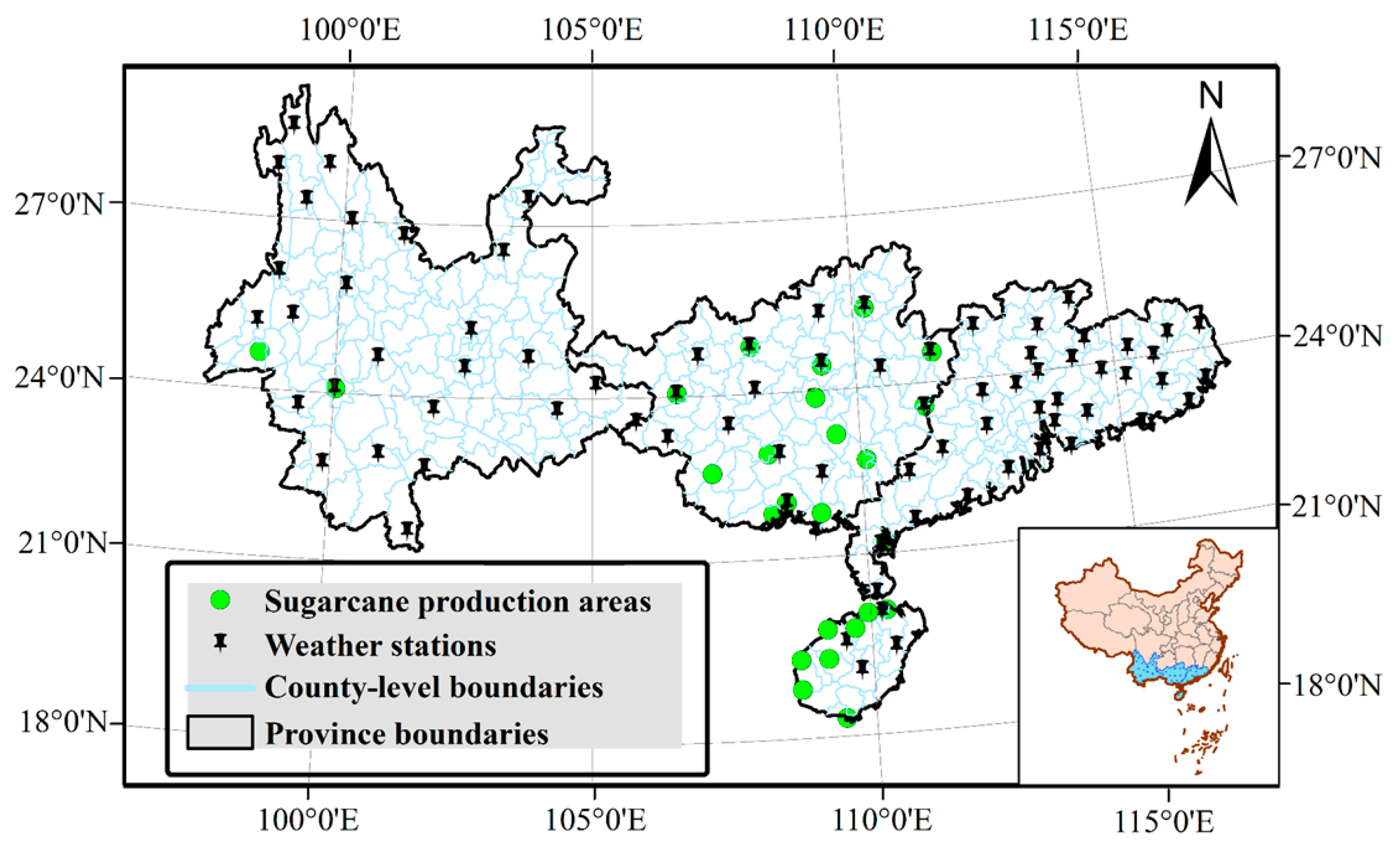
2.1. Sugarcane Study Area

In this study, 19 cities are selected as target production areas in four major sugarcane-producing provinces in southern China (18–30° N), including Guangxi, Guangdong, Yunnan, and Hainan provinces, as shown in Figure 1. During the sugarcane growing season, the average maximum temperature in the region is from 24.97 °C to 32.26 °C, the average minimum temperature is from 14.97 °C to 25.75 °C, and total precipitation is from 487.17 mm to 2914.4 mm. According to the statistical yearbook of provincial governments, the data on sugarcane yield and planting area in 15 years from 2005 to 2019 are collected to form a dataset. Sugarcane is divided into sugar cane and fruit cane according to the type of sugar cane because the area planted with fruit cane is small and no valid data can be formed. In addition, fruit cane shape and unit weight differ from sugar cane, which can interfere with the unit yield in the data set. Therefore, the planting area and planting yield of fruit sugarcane are screened, and only sugarcane data are counted. In the paper, Matlab (MathWorks, Natick, MA, USA) is applied for simulation application calculations.

2.2. Meteorological and Soil Data Collection

In this study, the entire growth process of sugarcane was divided into four cycles: seeding stage, germination tillering stage, elongation stage, and maturation stage. Meteorological and soil information was mainly counted in each cycle. Table 1 lists the meteorological and soil input variables required to build the model. Among them, the temperature and precipitation in the meteorological data are mainly from the statistics of some meteorological stations and the website of NOAA-NCEI. Wind speed and sunshine intensity data are from the dataset of ECMWF Re-Analysis 5 (ERA5) monthly averaged data on single levels from 1979 to the present [25]. ERA5 is the fifth generation of the ECMWF reanalysis of global climate and weather values over the past 40 to 70 years. This dataset counts each month’s information at a spatial resolution of 0.25° × 0.25°, and then forms the input data of this research model after cumulative processing. Soil data are derived from a GLDAS, which was developed jointly by GSFC and NECP in the United States [26,27]; the system has a spatial resolution of 0.25° × 0.25° and a temporal resolution of month by month. The selected data are processed by accumulating and averaging to generate the input for the model. The original dataset sources are all real data between 2005 and 2019. Based on the original data set, 270 groups of sample values are obtained by filtering null values and outliers. We consider selecting 230 sets of samples as the training set and the remaining 40 sets as the test set. The variation range of input variables is shown in Table 2. In addition, the effective accumulated temperature refers to the sum of the effective temperature of crops in the whole growth period, that is, the sum of the difference between the daily average temperature T and biological zero θ of crops in a certain period of time (n days). In this study, the biological temperature of sugarcane is set at 10 °C, and the effective accumulated temperature Y is calculated from temperature-related data using the following equation:
Y n = i = 1 n T i θ

2.3. Model Descriptions

In this study, in order to obtain the algorithm with the highest prediction accuracy and the best generalization capability, we choose BP neural network, random forest machine learning, and least square support vector machine to compare three algorithms and optimize the parameters of the algorithm with the best performance to find the optimal value of the model. In addition, RMSE, MAE, MAPE, R2, and SMAPE are used to evaluate the generalization ability and prediction accuracy of each model.
R M S E = 1 n i = 1 n y i y ^ i 2
M A E = 1 n i = 1 n y i y ^ i
R 2 = 1 1 n y i y ^ i 2 1 n y i y ¯ i 2
M A P E = 100 % n i = 1 n y i y ^ i y i
S M A P E = 100 % n i = 1 n y i y i ^ y i ^ + y i 2

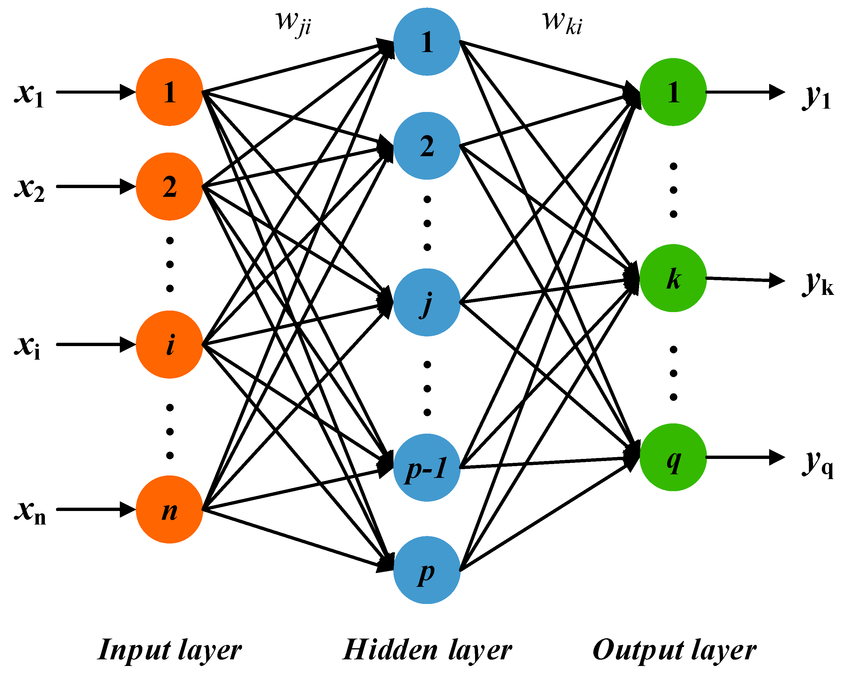
2.3.1. Back Propagation Neural Network (BPNN)

BPNN is a basic neural network, first proposed by Rumelhart and McClelland in 1986 [28]. It is characterized by the forward propagation of signals and backward transmission of errors. The information is forward propagated through layer-to-layer connections, and the error is back-propagated and weights are updated through a back-propagation algorithm to minimize the error between the predicted output and the actual output. BPNN has the advantages of feature extraction by learning, memory association, parallel architecture, autonomous learning, and self-adaptive ability [29], and BPNN models have been widely used in precipitation forecasting, meteorological parameter rainfall forecasting studies [30], regional surface soil moisture estimation [31], etc.
The topological structure of BPNN is shown in Figure 2, which consists of the input layer, hidden layer, and output layer. The connections between neurons of each layer are formed by weights and thresholds. The weight and threshold are constantly adjusted by the gradient descent method to minimize the error between the network output value and the expected value [32]. The BPNN works in two steps: the first step is the forward propagation of the signal, and the value of the output layer is calculated from the input layer using the kernel function of the hidden layer; the second step is the back propagation of errors. The output errors are transmitted back from the hidden layer to the input layer and distributed to each neuron. According to the prediction error, the weight and threshold between the hidden layer node and the output node is adjusted, and the expected value is finally reached. The process expressions of H calculation of hidden layer output (Formula (7)), O calculation of output layer output (Formula (8)), weight ω i j and ω j k update (Formulas (10) and (11)), hidden layer threshold a, and output layer threshold b update (Formulas (12) and (13)) are as follows:
H j = f i = 1 n ω i j x i a j   j = 1,2 , , l
O k = j = 1 l H j ω j k b k   k = 1,2 , , m
e k = Y k O k
ω i j = ω i j + η H j 1 H j x i k = 1 m ω j k e k   i = 1,2 , , n ; j = 1,2 , , l
ω j k = ω j k + η H j e k   j = 1,2 , , l ; k = 1,2 , , m
a j = a j + η H j 1 H j k = 1 m ω j k e k   j = 1,2 , , l
b k = b k + e k   k = 1,2 , , m
where f is the implied layer excitation function, n is the number of input nodes, m is the number of output nodes, l is the number of implied layer nodes, e is the network prediction error, and η is the learning rate.

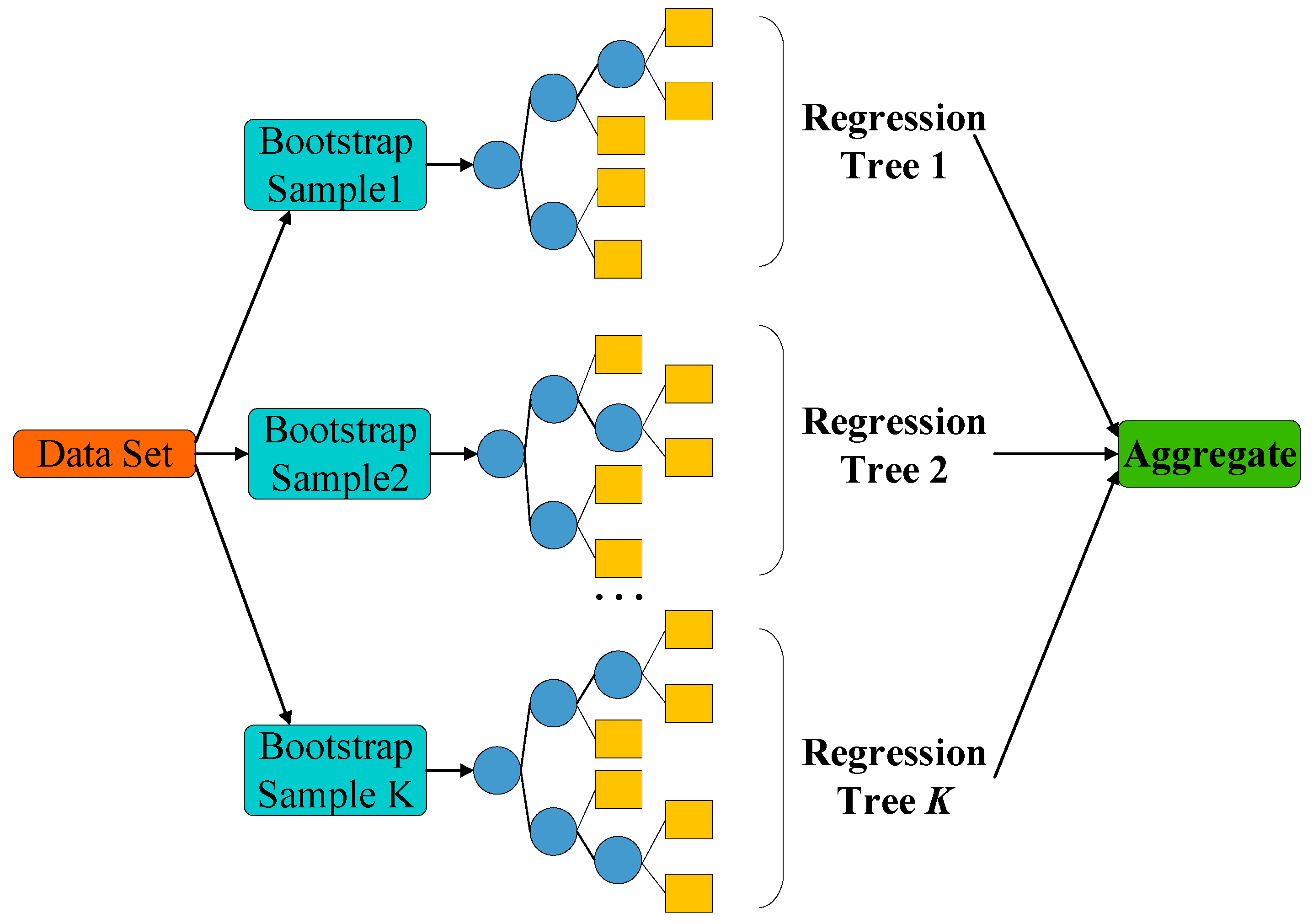
2.3.2. Random Forest (RF)

Random forest is an algorithm that integrates multiple decision trees for regression or classification through integrated learning techniques [33]. The advantage of the Random forest algorithm is that it can determine the importance of features without feature selection and analyze the interaction between different features. In addition, for unbalanced datasets, the Random forest algorithm can balance the error and maintain the model accuracy. In the Random Forest regression, each decision tree is considered as a basic unit that selects a portion of a branch of the dataset by setting a threshold. Essentially, Random forest is a classifier integration algorithm based on decision trees, each of which relies on independently distributed random vectors. Random forest generates multiple classification trees by randomly observing column vectors and row vectors and finally summarizes the results of each classification tree. In order to obtain optimal segmentation in generating random forests, the number of decision trees and the number of variables need to be selected and tested. Different from the single decision tree model, RF is based on the Bootstrap method of repeated sampling in the original dataset S n to generate multiple new datasets ( S n l ) of equal capacity to the original dataset. Then, the decision tree is constructed by randomly selecting the split attribute set, and the predictions of multiple decision trees are integrated, and the final prediction result is obtained through voting. The prediction result depends on the average result of the decision tree (Figure 3). The model is represented as follows:
Y ^ = 1 q l = 1 q h ^ X , S n l
where q denotes the number of decision trees.

2.3.3. Least Squares Support Vector Machine (LSSVM)

SVM is a machine learning (ML) method that can be used for classification and regression, which was proposed by Vapnik and Cortes [34]. Support vector machine achieves pattern recognition between two-point classes by looking for decision surfaces determined by certain points of the training set, called support vectors. It has good fitting accuracy and speed when processing nonlinear data, and is suitable for small sample research. The goal of SVM is to create a classification hyperplane, separate the two types, and maximize the isolation edge. Then, Sukens et al. proposed LSSVM [35,36,37], which uses the least square linear system as the loss function, and the inequality constraints of the optimization problem are converted into equality constraints, so as to obtain better performance than SVM.
LSSVM maps nonlinear problems to linear problems in a high-dimensional space. For a given nonlinear training sample data, N is the number of samples, and the linear regression function is constructed as follows:
f x = ω T φ x + b
where ω T is the column vector of power coefficients in the high-dimensional feature space; b is the deviation; and φ x is the nonlinear mapping. The solution of the linear regression function is transformed into the following optimization problem:
m i n ω , ξ 1 2 ω 2 + γ 2 τ = 1 N ξ 2   y i ω T φ x i + b = 1 ξ i ,   i = 1,2 , N
where γ > 0 is the penalty coefficient and ξ i is the error variable. The above formula is substituted into the Lagrange function:
L ω , b , ξ , b = 1 2 ω 2 + γ 2 τ = 1 N ξ i 2 k = 1 N a i y i ω T φ x i + b 1 + ξ i
where a i   > 0 is the Lagrange multiplier. Finally, the kernel function is set as K ( x i , x j ) , and the optimal regression function is obtained by solving the KKT optimization condition:
f x = i = 1 l a i y i K x i , x j + b

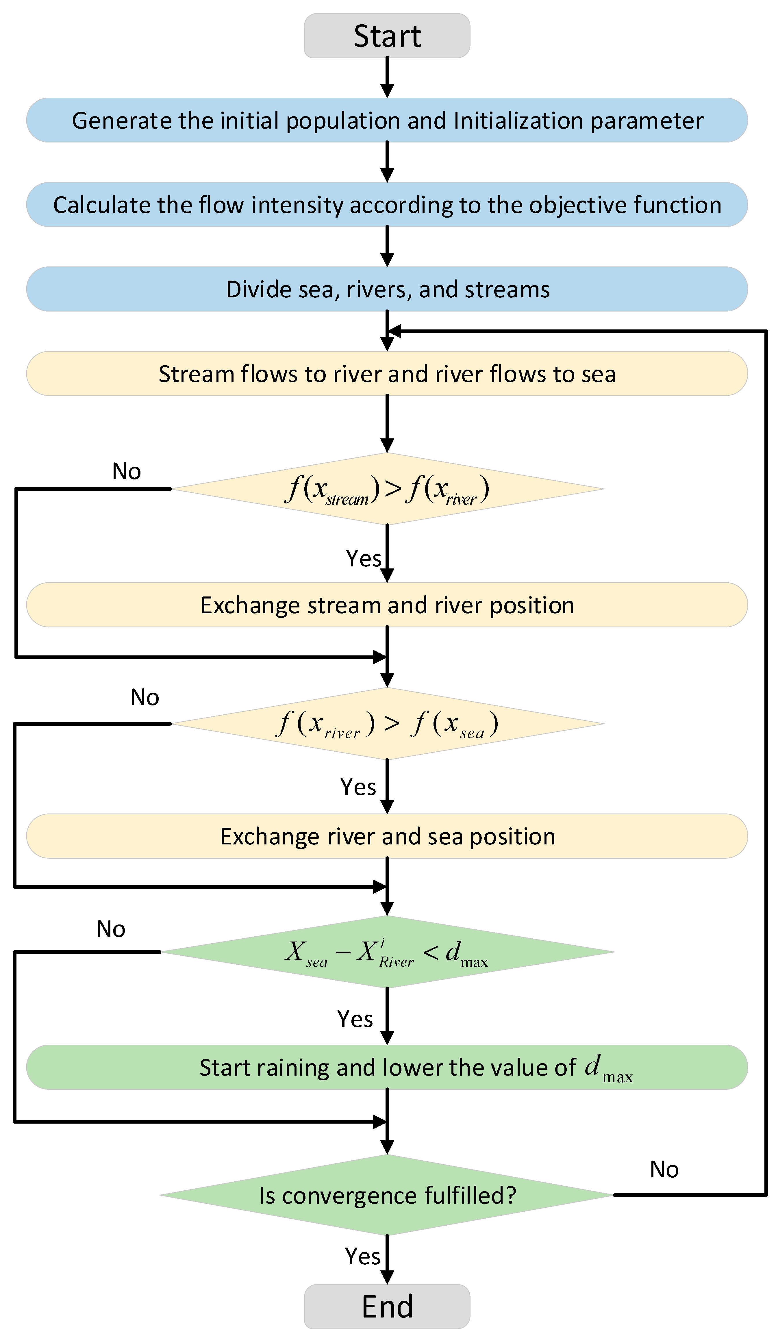
2.3.4. Water Cycle Algorithm (WCA)

In order to further improve the accuracy of the prediction model, optimization of the model parameters using an optimization-seeking algorithm is necessary. WCA is a new robust search method, which is a meta-heuristic algorithm proposed by Hadi Eskandar et al. in 2012 inspired by the natural water cycle process [38]. In the process of the water cycle, assuming that precipitation occurs constantly, the individuals generated by rain constitute the population of the algorithm, which is divided into three levels according to flow intensity. The best level is the ocean, the second level is the river, and the rest are streams. The individual composition of the algorithm is as follows:
The population initialization simulates the natural rainfall process. To meet the randomness of the rainfall process, WCA uses a random function to arrive at the initial population ( X ), and it can be expressed as follows:
X = L B + r a n d × ( U B L B )
where L B and U B represent the lower and upper bounds of the population, respectively. Moreover, r a n d denotes a vector generated randomly between 0 and 1 . In addition, the matrix expression of the population is as follows:
X = R a i n d r o p 1 R a i n d r o p 2 R a i n d r o p 3 R a i n d r o p N = S e a R i v e r 1 R i v e r 2 R i v e r N s r S t r e a m N s r + 1 S t r e a m N s r + 2 S t r e a m N p o p = x 1 1 x 2 1 x N 1 x 1 2 x 2 2 x N 2 x 1 N p o p x 2 N p o p x N N p o p
where N p o p is the number of populations and N is the dimension of the search space. After forming the initial population, each individual is brought into the objective function to calculate the traffic intensity for ranking.
C o s t = f x 1 1 , x 1 1 , x 1 1 , , x 1 1   i = 1,2 , , N p o p
N s r = N u m b e r   o f   R i v e r s + 1
N s t r e a m = N p o p N s r
In the above equation, N s r is the number of rivers and oceans, N s t r e a m is the number of streams, and the number of streams flowing into oceans/rivers is obtained using the following equation:
N s r n = r o u n d C n n = 1 N s r C n × N s t r e a m , n = 1,2 , , N s r
C n = C o s t n C o s t N s r + 1
After the initial population is formed and graded, the confluence begins; that is, the algorithm enters an iterative process, and the location of rivers and oceans is constantly updated, as described below:
X S t r e a m t + 1 = X S t r e a m t + r a n d × C × X R i v e r t X S t r e a m t
X S t r e a m t + 1 = X S t r e a m t + r a n d × C × X S e a t X S t r e a m t
X R i v e r t + 1 = X R i v e r t + r a n d × C × X S e a t X R i v e r t
where rand is a random number that meets uniform distribution between (0, 1), and C is the updated coefficient between (1, 2), which is generally set to 2.
All optimization algorithms need to consider the problem of falling into local optimization due to fast convergence. WCA can solve the local optimization problem by introducing an evaporation process and rainfall process to enhance the searchability of the algorithm. Therefore, rivers and streams are properly examined using the following equation to determine if they are close enough to the sea to influence the evaporation process:
X S e a X R i v e r < d m a x
d m a x i + 1 = d m a x i d m a x i M a x   I t e r a t i o n
where the initial value of d m a x is a constant close to 0, and the value in this study is 10 16 . When the above formula is true, that is, when evaporation conditions are met, the real-time rainfall process and the formation of new streams can be determined by the following equation:
X S t r e a m N e w = L B + r a n d × U B L B
where UB and LB are the upper and lower boundaries of the search space, respectively.
Algorithm 1 is the pseudo-code for the WCA:
Algorithm 1 Pseudo-code of WCA
Initialize parameters: N p o p , N s r , d m a x , M a x   I t e r a t i o n ;
Randomly initialize the population X by Equation (19);
Calculate the fitness value C o s t of the population by Equation (21);
Sort the population in ascending order by fitness value;
Divide the population into three categories: X S e a , X R i v e r , X S t r e a m ;
Calculate the number of streams flowing into a river or ocean N s r n by Equation (24);
while  I t e r a t i o n < M a x   I t e r a t i o n  do
Allocate streams moving to sea and generate new stream X n e w s t r e a m by Equation (27);
if  C o s t ( X n e w s t r e a m ) < C o s t ( X s e a )  then
Swap X s e a and X n e w s t r e a m ;
end if
Allocate streams moving to river and generate new stream X n e w s t r e a m by Equation (26);
if  C o s t ( X n e w s t r e a m ) < C o s t ( X r i v e r )  then
Swap X r i v e r and X n e w s t r e a m ;
end if
Allocate rivers moving to sea and generate new river X n e w r i v e r by Equation (28);
if  C o s t ( X n e w r i v e r ) < C o s t ( X s e a )  then
Swap X s e a and X n e w r i v e r ;
end if
Check the evaporation to generate new streams X n e w s t r e a m by Equation (31);
Decrease d m a x by Equation (30);
I n t e r a t i o n = I t e r a t i o n + 1
end while
return  X s e a
The WCA optimization process is shown in the flow chart (Figure 4):

2.3.5. Variance-Based Sensitivity Analysis

In sensitivity analysis, any model may be viewed as a function Y = f ( X ) , where X is a vector of d uncertain model inputs X 1 , X 2 ,     X d , and Y is a chosen univariate model output (note that this approach examines scalar model outputs, but multiple outputs can be analyzed via multiple independent sensitivity analyses). Furthermore, it is assumed that the inputs are independently and uniformly distributed within the unit hypercube, i.e., X i 0 ,   1 for i = 1 ,   2 , d . This incurs no loss of generality because any input space can be transformed onto this unit hypercube. f(X) may be decomposed in the following way:
Y = f 0 + i = 1 d f i ( X i ) + i < j d f i j ( X i , X j ) + + f 1,2 , d ( X 1 , X 2 , , X d )
where f 0 is a constant and f i is a function of X i , X j a function of X i and X j , etc. A condition of this decomposition is as follows:
0 1 f i 1 i 2 i s ( X i 1 , X i 2 , , X i s ) d X k = 0 ,   f o r   k = i 1 ,     , i s
i.e., all the terms in the functional decomposition are orthogonal. This leads to definitions of the terms of the functional decomposition in terms of conditional expected values:
f 0 = E ( Y )
f i ( X i ) = E ( Y | X i ) f 0
f i j ( X i , X j ) = E ( Y | X i , X j ) f 0 f i f j
From this, it can be seen that f i is the effect of varying X i alone (known as the main effect of X i ), and f i j is the effect of varying X i and X j simultaneously, in addition to the effect of their individual variations. This is known as a second-order interaction. Higher-order terms have analogous definitions.
Now, further assuming that the f ( X ) is square-integrable, the functional decomposition may be squared and integrated to provide the following:
f 2 ( X ) d X f 0 2 = s = 1 d i 1 <   < i s d f i 1     i s 2 d X i 1     d X i s
Notice that the left-hand side is equal to the variance of Y , and the terms of the right-hand side are variance terms, now decomposed with respect to sets of the X i . This finally leads to the decomposition of variance expression:
V a r ( Y ) = i = 1 d V i + i < j d V i j + + V 12     d
V i = V a r X i ( E X ~ i ( Y | X i ) )
V i j = V a r X i j ( E X ~ i j ( Y | X i , X j ) ) V i V j
The X ~ i notation indicates the set of all variables except X i . The above variance decomposition shows how the variance of the model output can be decomposed into terms attributable to each input, as well as the interaction effects between them. Together, all terms sum to the total variance of the model output.
A direct variance-based measure of sensitivity S i , called the “first-order sensitivity index”, or “main effect index”, is stated as follows:
S i = V i V a r ( Y )
This is a contribution to the output variance of the main effect of X i ; therefore, it measures the effect of varying X i alone, but averaged over variations in other input parameters. It is standardized by the total variance to provide a fractional contribution. Higher-order interaction indices, S i j , S i j k , and so on, can be formed by dividing other terms in the variance decomposition by V a r ( Y ) . Note that this has the following implication:
i = 1 d S i + i < j d S i j + + S 12     d = 1
Using the S i , S i j and higher-order indices given above, one can build a picture of the importance of each variable in determining the output variance. However, when the number of variables is large, this requires the evaluation of 2d−1 indices, which can be too computationally demanding. For this reason, a measure known as the “Total-effect index” or “Total-order index”, S T i , is used. This measures the contribution to the output variance of X i , including all variance caused by its interactions, of any order, with any other input variables. It is given as follows:
i = 1 d S T i 1
Due to the fact that the interaction effect between, e.g., X i and X j is counted in both S T i and S T j . In fact, the sum of the S T i will only be equal to 1 when the model is purely additive.

3. Result and Discussion

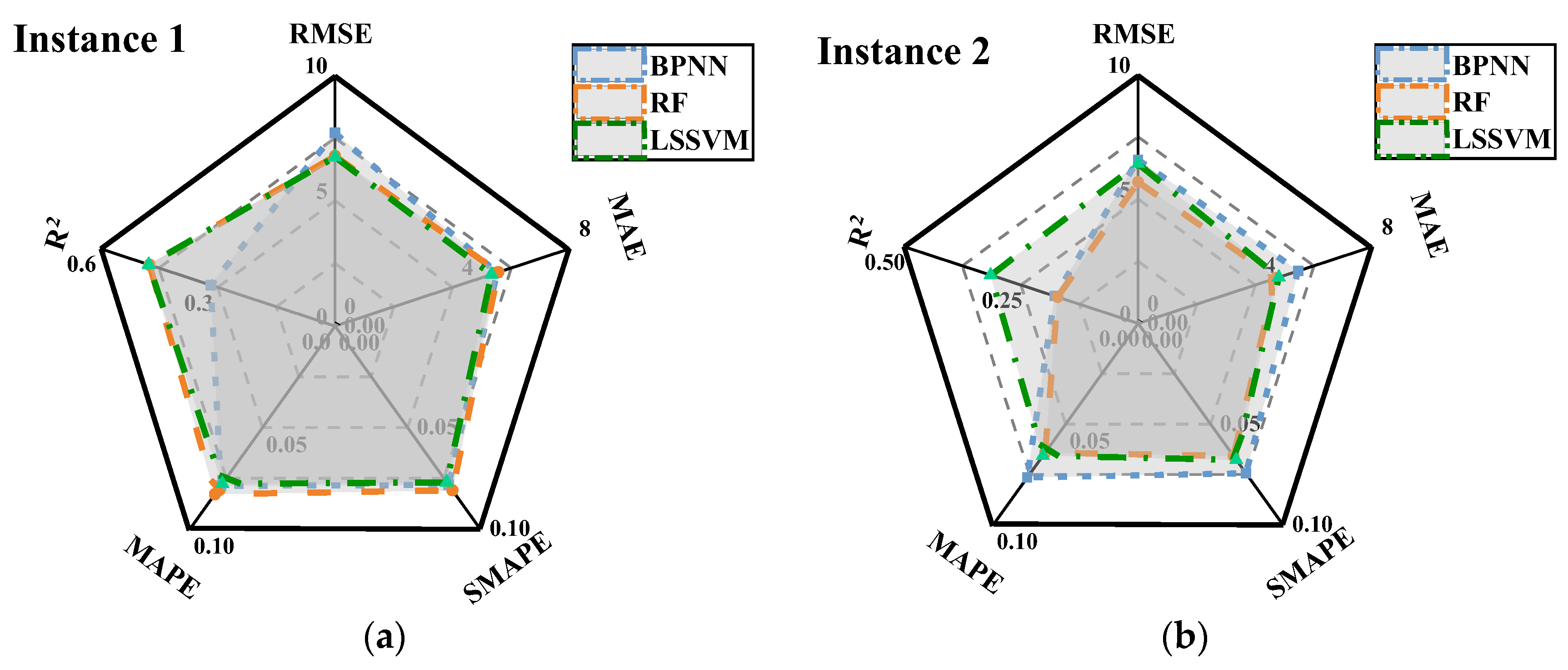
3.1. Models Performance

In this study, environmental variables (climate and soil factors) are used as inputs, and the unit yield of sugarcane is used as outputs to construct a prediction model. Based on the original data set, 270 groups of sample values are obtained by filtering null values and outliers. We consider selecting 230 sets of samples as the training set and the remaining 40 sets as the test set. The training and testing sets represent 85% and 15% of the entire dataset, respectively. And the model is applied to two instances, the main difference between these two instances is in dividing the samples, and the test set samples are selected differently. The test set of the first instance is selected from the dataset with equal variances, and the samples are selected mainly to verify the accuracy of the model with time differences, that is, to predict the data of the remaining 2 years based on the data of 13 years in each place. The test set of the second instance is selected from the last 40 samples of the dataset to verify the accuracy of the model with regional differences, that is, to predict the data of the remaining 2 regions with the data of 17 regions. The validity of the model in a certain range of time and space is verified by different divisions.
In the process of modeling, we randomly sample the dataset and carry out ten-fold cross-validation to reasonably balance the running time and accuracy of the prediction model, reduce the contingency caused by the single division of the training set and validation set, and avoid selecting models without generalization ability due to special division.
According to the above model construction method, BPNN, RF, and LSSVM of machine learning algorithm are used to construct prediction models, respectively, and five evaluation indexes, RMSE, MAE, R2, SMAPE, and MAPE, are used to compare the advantages and disadvantages of various algorithms. The calculation results are shown in Figure 5. In instance 1 (Figure 5a), the RMSE of three algorithms are approximated with the estimated error values ranging from 6 to 7.5 ton/ha, while R2 of LSSVM is 40.79% and 3.97% higher than BPNN and RF, respectively, indicating a higher degree of fitting of LSSVM algorithm. In instance 2 (Figure 5b), though the RMSE value of LSSVM is slightly larger than that of RF, its R2 is 76.96% and 83.13% higher than that of the other two models. Combined with the two graphs, the model constructed by the LSSVM algorithm has higher prediction accuracy and generalization ability and is more suitable for sugarcane yield prediction.
Another thing that needs to be explained is that by comparing the two Figure 5a,b, it is found that the prediction model fit (R2) for studying geographical differences is generally poor, which may be due to the fact that the geographical span leads to large differences in raw data such as climatic factors and soil factors, making the raw data highly random and volatile, and the singular values are not easily detected, which brings challenges to the stability and accuracy of the prediction model.

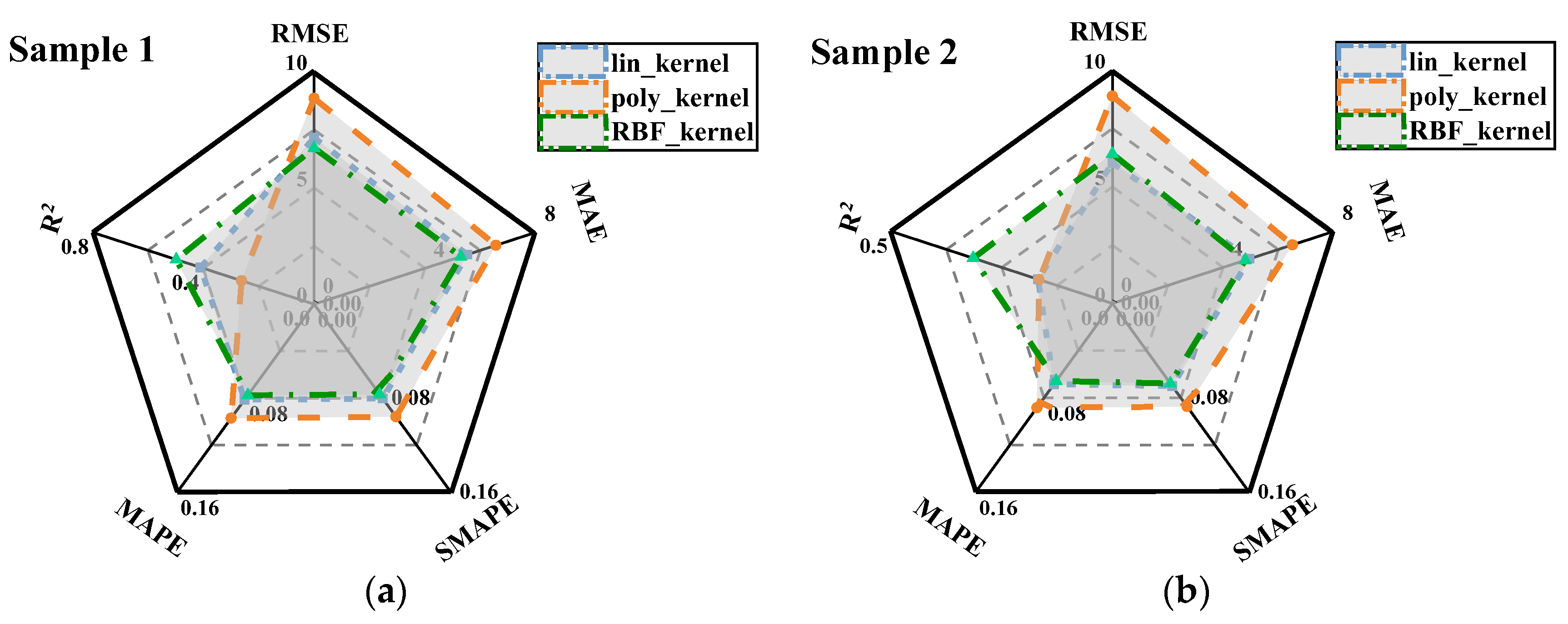
3.2. Comparison of LSSVM Models with Different Kernel Functions

Compared with other algorithms, LSSVM has higher accuracy and generalization ability, so this study uses the prediction model constructed by LSSVM. LSSVM algorithm transforms data into high-dimensional space by introducing kernel function, which makes data linearly separable, reduces misclassified data points, and increases the generalization ability of the model. In this study, linear kernel function, polynomial kernel function, and Gaussian radial basis kernel function are applied to support vector machines to evaluate the prediction ability of the model. The expressions of each kernel function are as follows:
Linear kernel function (lin_kernel):
K x , μ = x T · μ
Polynomial kernel function (poly_kernel):
K x , μ = a x T μ + c q ,   q > 0
Gaussian radial basis kernel function (RBF_kernel):
  K x , μ = exp x μ 2 σ 2
The final results of each model are shown in Figure 6, where it can be seen that the R2 corresponding to the lin_kernel, poly_kernel, and RBF_kernel in instance 1 are 0.4098, 0.2622, and 0.6629, respectively, and the RMSE are 7.158, 8.852, and 5.534, respectively. The R2 comparison of three kernel functions in instance 2 is 0.1679, 0.1657, and 0.3147, respectively, and RMSE is 4.962, 6.509, and 4.803, respectively. In conclusion, RBF_kernel has higher prediction performance, and RBF kernel function is superior to other functions in terms of fit degree, fitting error, and generalization ability of the model.

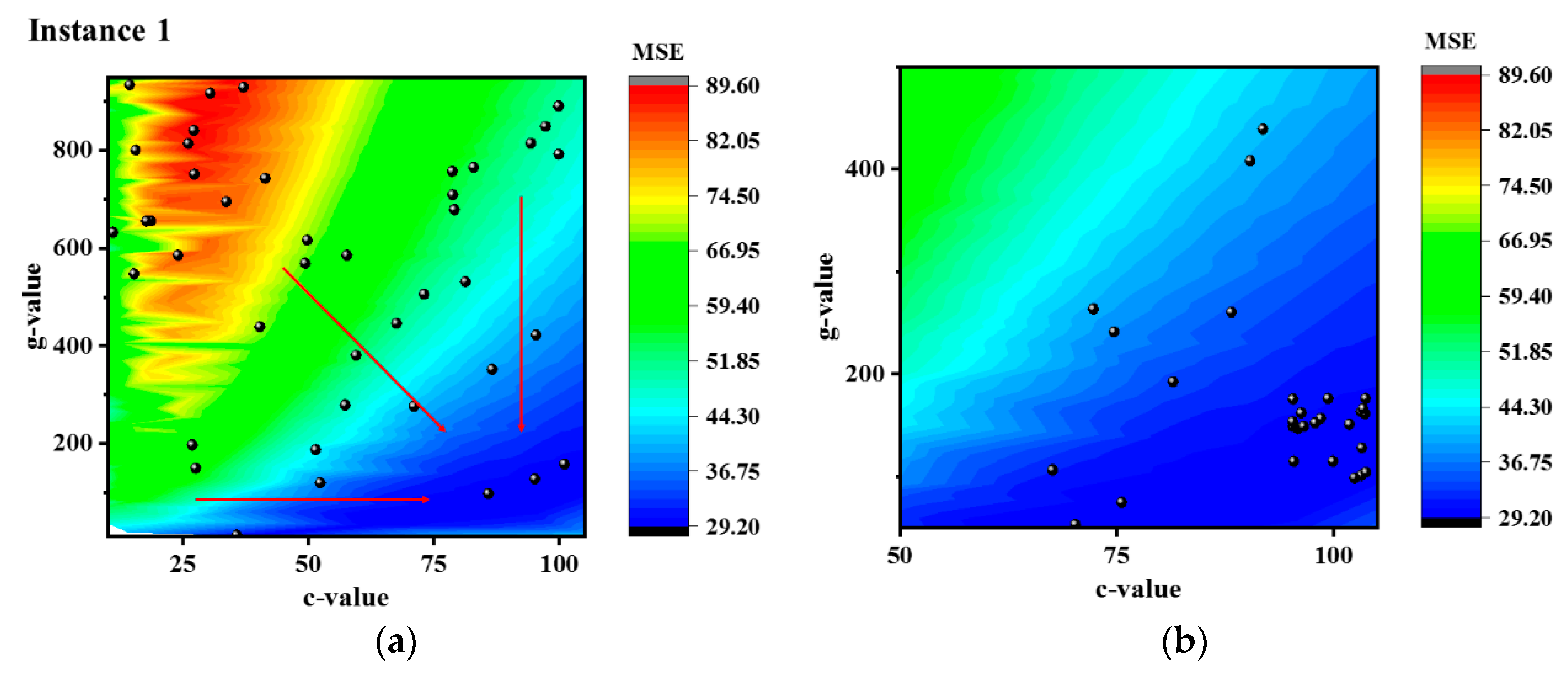
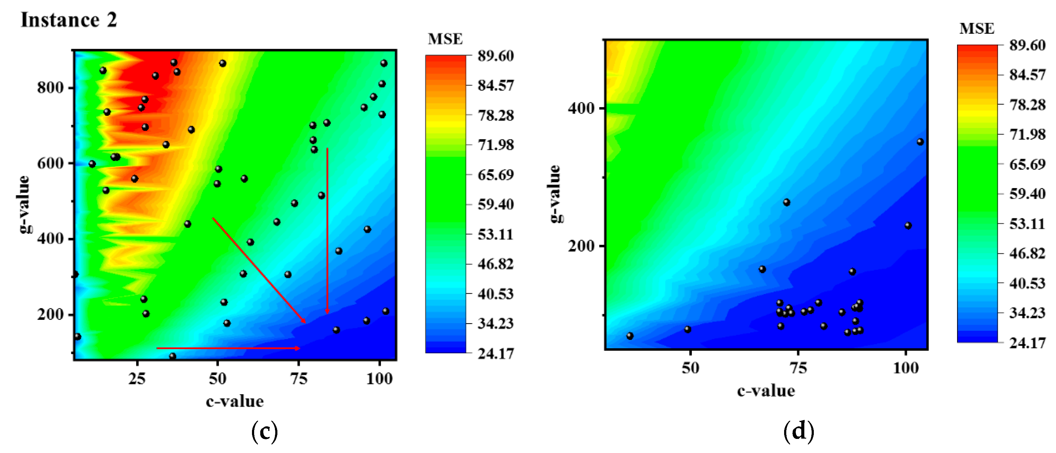
3.3. WCA Optimization Results

After determining the use of the LSSVM prediction algorithm and radial basis kernel function, the prediction accuracy of the LSSVM algorithm is closely related to the penalty value c and gamma value g in the kernel function. Among them, penalty value c is used to control the balance between margin maximization and error minimization, and gamma value g affects the mapping from sample space to feature space. Therefore, how to select c and g to optimize the prediction ability of the model needs special study.
In the past, the values of C and g were usually derived directly from experience [39]. In this paper, WCA is adopted to optimize the selection of two parameters by taking the error value of the sugarcane prediction model MSE as the fitness function.
Figure 7 shows the process and results of applying the water cycle algorithm to find the best for each of the two instances. At first, WCA forms populations via the rainfall process, uniformly and randomly distributed in the two-dimensional plane formed by the c and g values, and then forms location updates via the confluence processes such as streams flowing into rivers and rivers flowing into the ocean, causing the population value (c, g) to move toward the minimum value of MSE in the set range and eventually gather around the minimum value. The c value range is set to (1,110) and the g value range is set to (1,1000). Figure 7a,c show the distribution of the population in the c-g two-dimensional plane after generating the initial population. Figure 7b,d show that the original population gathers near the optimal value of the model via the continuous iterative updating of the position after water cycle optimization. The final results show that the optimal value of instance 1 is clustered around (105,115.798), and that of Instance 2 is clustered around (78.428,80).

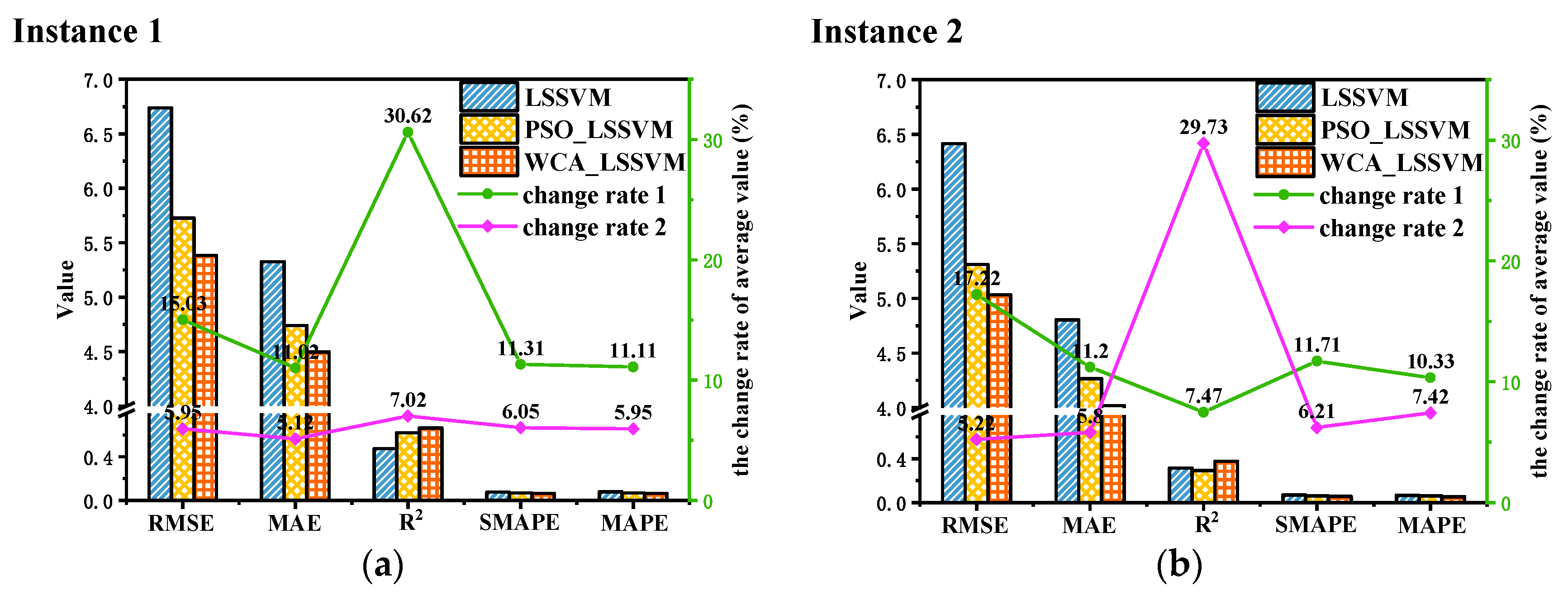
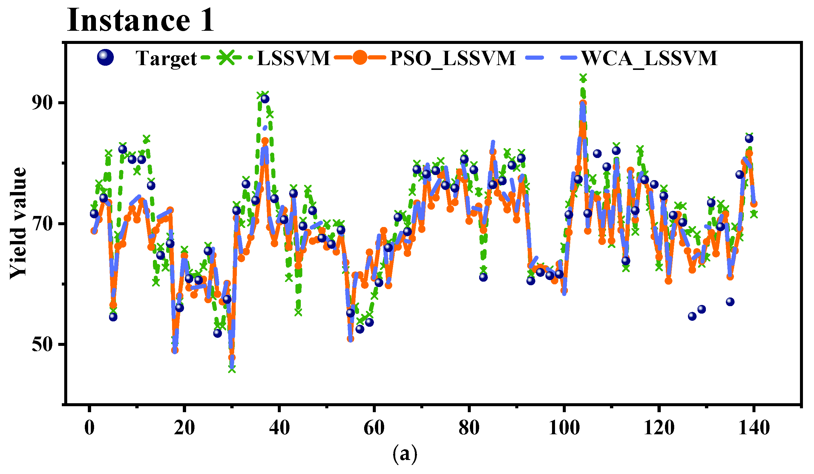
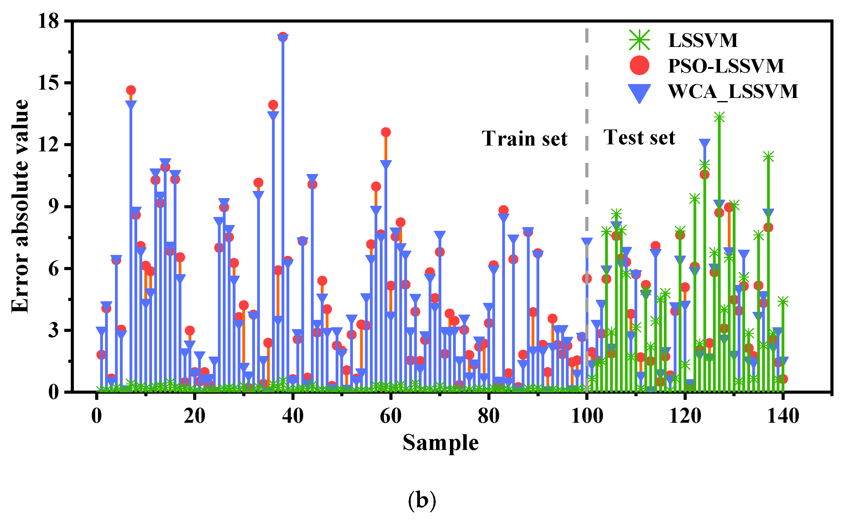
3.4. WCA-LSSVM Model Performance

In this study, the LSSVM algorithm optimized by WCA (WCA-LSSVM) is used to predict sugarcane yield. To verify the effectiveness of the proposed model, we build the LSSVM model without optimization and the LSSVM model with particle swarm optimization (PSO-LSSVM), and then apply the three models to two instances to compare the prediction accuracy and fitting ability of the different models.
The comparison results of the three models are shown in Figure 8. Among them, change rate 1 is the rate of change in WCA-LSSVM with respect to each indicator of LSSVM, and change rate 2 is the rate of change in WCA-LSSVM with respect to each indicator of PSO-LSSVM. In Figure 8a, WCA-LSSVM shows a significant improvement in all indicators compared with LSSVM, especially in terms of model accuracy and fit degree. RMSE decreased from 6.716 to 5.385, R2 increased from 0.497 to 0.665, and the change rates reached 15.03% and 30.62%, respectively. Compared with PSO-LSSVM, WCA-LSSVM also has a slight improvement in each index, with an increase of 5–7%. In Figure 8b, compared with LSSVM, WCA mainly improved the accuracy of the model, with RMSE, MAE, and SMAPE dropping from 6.414, 4.803, and 0.0678 to 5.032, 4.017, and 0.0561, respectively. And RMSE had the largest change rate, reaching 17.22%. Compared with PSO-LSSVM, WCA-LSSVM greatly improved the fitting accuracy of the model. R2 was improved from 0.291 to 0.378, with an increase of 29.73%. Other indicators were also improved at different ranges, with an increase of 5–8%. Therefore, combined with Figure 8 and Table 3, it can be seen that WCA-LSSVM has a good improvement in both the error accuracy and the fitting degree of the model.
Table 3 is a comparison of the five evaluation indicators of different models. R2 (Determination Coefficient) and RMSE (Root Mean Square of Error) are the most commonly used metrics for evaluating the performance of a predictive model. The closer R2 is to 1, the better the fit of the predictive model; the smaller RMSE is, the higher the predictive accuracy of the model. Moreover, MAE (Mean Absolute Error), MAPE (Mean Absolute Percent Error), and SMAPE (Symmetric Mean Absolute Percentage Error) are also effective indicators for evaluating the prediction accuracy of models. It can be seen that the prediction performance of the WCA_LSSVM prediction model is superior to other comparative models. Simultaneously, among other prediction models applied to sugarcane production areas in Guangxi [40], the lowest RMSE value is 10.34 and the lowest MAPE value is 0.0685. In comparison, it is evident that the WCA_LSSVM prediction model proposed in this article surpasses others applied to the Guangxi sugarcane production area in terms of prediction accuracy. In Figure 9 and Figure 10, Figure 9a and Figure 10a show the intuitive comparison between the output value predicted by each algorithm and the real value, Figure 9b and Figure 10b show the absolute value of the error of the model. In addition, we introduce relative error (RE), that is, the percentage of absolute error in the true value, to intuitively show the prediction level of each model. The calculation formula is as follows:
R E % = y i ^ y i y i × 100
where y i ^ is the predicted value of the model output and y i is the true value. The calculation results are shown in Table 4.
In Figure 9 and Table 4, it can be seen that LSSVM has better error accuracy and fitting accuracy when training data, RMSE can reach 0.1507, but when testing the set prediction, LSSVM has the largest prediction error and the worst fitting degree, with the maximum relative error reaching 27%. This may be because it produces the overfitting in the previous training, leading to the prediction effect not being ideal. In Figure 9b, it can be seen intuitively that both PSO-LSSVM and WCA-LSSVM performed better than LSSVM in the test, but the absolute error value of WCA-LSSVM accounted for 95% in the range [0, 10], with a maximum value of 12.75, while the absolute error value of PSO-LSSVM reached a maximum value of 15.86. And RE of WCA-LSSVM is basically controlled within 15%, which has higher prediction accuracy.
In Figure 10 and Table 4, the prediction curve of instance 2 is described. It can be seen that for the training data PSO-LSSVM, it is difficult to effectively follow the target value, the fitting degree is poor. Its absolute error value is much higher than LSSVM and WCA-LSSVM. The maximum absolute error value is 17.648, and the training effect is lower than the other two algorithms. However, in the test set verification results of the model, the prediction curve of LSSVM fluctuates greatly, and the prediction effect is not as good as PSO-LSSVM and WCA-LSSVM. In addition, the absolute error of WCA-LSSVM is basically controlled within 10, while the maximum absolute error of LSSVM and PSO-LSSVM is 13.87 and 11.99. Combining the tables, the error values of the three models of LSSVM, PSO-LSSVM, and WCA-LSSVM in the interval of RE < 5% account for 42.5%, 50%, and 55%. Moreover, the maximum relative error of LSSVM is 28.789%, that of PSO_LSSVM is 16.701%, and that of WCA_LSSVM is all within 15%.
In summary, the comparison of various models shows that parameter optimization using WCA significantly improves the prediction accuracy and generalization ability of LSSVM, and makes the algorithm converge to the optimal value more easily. Compared with other models, WCA-LSSVM is more competitive and applicable for different times and locations within a certain range.

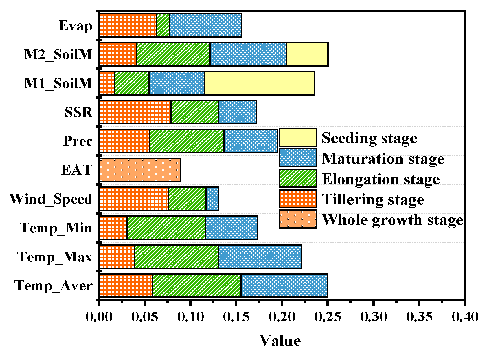
3.5. Sensitivity Analysis

Sensitivity analysis is to use a randomly generated sequence as the prediction input to fit the prediction model and calculate the influence degree of each parameter on the model output by the ratio of variance, which ultimately improves the accuracy and reliability of the sugarcane yield prediction model. The results are shown in Figure 11. The variables in the figure are divided according to the different growing stages of sugarcane and it can be seen that, firstly, temperature (average temperature, maximum temperature, and minimum temperature) has a decisive influence on sugarcane yield. Low temperatures and reduced rainfall can stress the growth rate of sugarcane at the length and maturity stages and reduce sugarcane yield. However, the minimum temperature had less effect on the growth of sugarcane in this study. This is attributed to the fact that the minimum temperature is higher than the biological zero of sugarcane almost all year round under the climatic conditions of Guangxi, so the effect is not as strong as other temperature factors in the sensitivity analysis. Variations in rainfall had a greater impact on the elongation stage of sugarcane growth, followed by the tillering stage, and had the least impact at the maturation stage. This is consistent with the study of sugarcane growth characteristics in Guangxi by Qin N et al. [41]. In terms of soil moisture, M1_SoilM and M2_SoilM correspond to soil moisture at 0–10 cm depth and soil moisture at 10–40 cm depth, respectively. It can be seen that M1_SoilM has a great influence in the seeding stage, and M2_SoilM has a higher influence in other stages after the seeding stage. This is because the growth of sugarcane is closely linked to the absorption of nutrients and water in the soil. Despite the fact that soil moisture fluctuates more significantly at the surface, the root distribution density of sugarcane is higher within the 10–40 cm depth range of soil [42], rendering it more vulnerable to variations in soil moisture, which can ultimately lead to alterations in yield. The variation in soil moisture was related to both total evapotranspiration and rainfall during the growth cycle. Total evapotranspiration during the growth cycle is shown in Figure 11, which has a large effect on the stage of tillering and maturation, but the change in total precipitation has a large effect on the elongation stage. This is attributed to the high water demand during the elongation stage of sugarcane growth, where the amount of water stored in the soil after precipitation is much higher than the evapotranspiration loss from the stems and leaves. In contrast, the total diffuse evapotranspiration of sugarcane at the leaf tillering and maturation stages is susceptible to variations in a number of factors and thus affects the growth process due to the high leaf area. The high effect of solar radiation intensity on the tillering stage is accounted for by the highly effective utilization of diffuse radiation by the high leaf area, which in turn results in the variation in sugarcane yield. Some of these conclusions have been summarized by other researchers [43,44,45], which also verified the validity of the prediction model in this paper.

4. Conclusions

This study collected environmental information from four provinces in Southern China and sugarcane yield data, preprocessed the original data via filtering outliers and normalized analysis, and different machine algorithms were selected to build prediction models for comparison. The best-performing LSSVM was selected, and the prediction model was applied to two instances after optimizing the LSSVM parameters using WCA. The results show that the model proposed in this paper can reach RMSE of 5.385 and 5.032 and MAPE of 0.0649 and 0.0545 when applied in two instances, whereas the lowest RMSE is 10.34 and the lowest MAPE is 0.0685 in the other models for the prediction of sugarcane yield in Guangxi. A comparison of this paper’s model is more accurate in predicting the sugarcane yield in Guangxi. Comparing the Particle Warm Optimization and Water Cycle Optimization methods, the RMSE values of the two instances after Particle Warm Optimization are 5.726 and 5.310, and the MAPE are 0.0691 and 0.0589, respectively. Despite the improvement in the accuracy, the effect is still not as effective as that of the Water Cycle Optimization algorithm. It can be seen that the model is more susceptible to converging to the optimal value when optimizing the model using the WCA optimization method, achieving a further improvement in accuracy.
In addition, the environmental variables of sugarcane growth are divided according to the growth stage, and the sensitivity of each variable is calculated by fitting the WCA-LSSVM prediction model. It was found that although the main influencing factors of sugarcane production were temperature and precipitation, which was the same as the results of other papers, soil moisture at different depths also had a great impact on crop yield. The investigation results of this paper are of great research significance for the prediction of sugarcane yield in the Guangxi region. Meanwhile, it can provide an important reference for the government to formulate relevant policies and a decision-making basis for farmers to guide sugarcane planting, so as to improve the yield and quality of sugarcane and promote the development of the sugarcane industry.
Nonetheless, the results of this study are highly dependent on climatic data and do not take into account the effects of disturbances such as soil nutrients, varietal improvement, technological advances, changes in cultivation management, and social factors on sugarcane production. All these factors can lead to bias in the prediction results of sugarcane yield. Therefore, more variables such as remotely sensed vegetation indices (e.g., NDVI, SAVI, GNDVI, etc.) need to be included in the consideration of input variables, and the correlations of all input variables need to be screened in order to optimize the predictive effectiveness of the model. Meanwhile, in order to further improve the accuracy of studying the effects of climate change on sugarcane yield in the Guangxi region, future research should incorporate a comprehensive simulation with factors such as environment, genetics (varieties), and management measures, such as adjusting the sowing time as well as management-to-management relationships. This will also provide a more comprehensive and scientific theoretical basis for improving the quantity and quality of sugarcane in sugarcane production areas.

Author Contributions

Conceptualization, Y.Z. and T.S.; methodology, W.G.; software, Y.Z. and T.S.; validation, W.G. and C.F.; formal analysis, M.P.; resources, M.P.; data curation, T.S.; writing—original draft preparation, Y.Z.; visualization, C.F.; supervision, M.P.; funding acquisition, M.P. All authors have read and agreed to the published version of the manuscript.

Funding

This research was funded by the Guangxi University Sugarcane Research Fund, grant number 2022GZB008; and the National Natural Science Foundation of China, grant number U23A202599.

Institutional Review Board Statement

Not applicable.

Informed Consent Statement

Not applicable.

Data Availability Statement

The datasets generated during and/or analyzed during the current study are available from the corresponding author upon reasonable request.

Conflicts of Interest

The authors declare no conflict of interest.

Nomenclature

R2Determination Coefficient
RMSERoot Mean Square Error
MAEMean Absolute Error
MAPEMean Absolute Percentage Error
SMAPESymmetric Mean Absolute Percentage Error
NOAANational Oceanic and Atmospheric Administration
NCEINational Centers for Environmental Information
ECMWFEuropean Centre for Medium-Range Weather Forecasts
ERA5ECMWF Re-Analysis 5
GLDASGlobal high-resolution Land Surface Simulation System
GSFCGoddard Space Flight Center
NCEPNational Centers for Environmental Prediction
BPNNBack Propagation Neural Network
RFRandom Forest
SVMSupport Vector Machine
MLMachine Learning
WCAWater cycle algorithm
LSSVMLeast squares support vector machine
PSO-LSSVMParticle Warm Optimization of LSSVM
WCA_LSSVMWCA of LSSVM

References

  1. Sindhu, R.; Gnansounou, E.; Binod, P.; Pandey, A. Bioconversion of sugarcane crop residue for value added products—An overview. Renew. Energy 2016, 98, 203–215. [Google Scholar] [CrossRef]
  2. Jiang, H.; Li, D.; Jing, W.; Xu, J.; Huang, J.; Yang, J.; Chen, S. Early season mapping of sugarcane by applying machine learning algorithms to Sentinel-1A/2 time series data: A case study in Zhanjiang City, China. Remote Sens. 2019, 11, 861. [Google Scholar] [CrossRef]
  3. Zhao, Y.; Chen, M.; Zhao, Z.; Yu, S. The antibiotic activity and mechanisms of sugarcane (Saccharum officinarum L.) bagasse extract against food-borne pathogens. Food Chem. 2015, 185, 112–118. [Google Scholar] [CrossRef] [PubMed]
  4. Raheem, A.; Zhao, M.; Dastyar, W.; Channa, A.Q.; Ji, G.; Zhang, Y. Parametric gasification process of sugarcane bagasse for syngas production. Int. J. Hydrog. Energy 2019, 44, 16234–16247. [Google Scholar] [CrossRef]
  5. Algayyim, S.J.M.; Yusaf, T.; Hamza, N.H.; Wandel, A.P.; Fattah, I.R.; Laimon, M.; Rahman, S.A. Sugarcane Biomass as a Source of Biofuel for Internal Combustion Engines (Ethanol and Acetone-Butanol-Ethanol): A Review of Economic Challenges. Energies 2022, 15, 8644. [Google Scholar] [CrossRef]
  6. Viana, J.L.; de Souza, J.L.M.; Hoshide, A.K.; de Oliveira, R.A.; de Abreu, D.C.; da Silva, W.M. Estimating Sugarcane Yield in a Subtropical Climate Using Climatic Variables and Soil Water Storage. Sustainability 2023, 15, 4360. [Google Scholar] [CrossRef]
  7. Jiang, R.; Wang, T.T.; Jin, S.H.A.O.; Sheng, G.U.O.; Wei, Z.H.U.; Yu, Y.J.; Chen, S.L.; Hatano, R. Modeling the biomass of energy crops: Descriptions, strengths and prospective. J. Integr. Agric. 2017, 16, 1197–1210. [Google Scholar] [CrossRef]
  8. Hu, S.; Shi, L.; Huang, K.; Zha, Y.; Hu, X.; Ye, H.; Yang, Q. Improvement of sugarcane crop simulation by SWAP-WOFOST model via data assimilation. Field Crops Res. 2019, 232, 49–61. [Google Scholar] [CrossRef]
  9. Inman-Bamber, N.G. A growth model for sugar-cane based on a simple carbon balance and the CERES-Maize water balance. South Afr. J. Plant Soil 1991, 8, 93–99. [Google Scholar] [CrossRef]
  10. Jagtap, S.T.; Phasinam, K.; Kassanuk, T.; Jha, S.S.; Ghosh, T.; Thakar, C.M. Towards application of various machine learning techniques in agriculture. Mater. Today Proc. 2022, 51, 793–797. [Google Scholar] [CrossRef]
  11. Zhu, L.; Liu, X.; Wang, Z.; Tian, L. High-precision sugarcane yield prediction by integrating 10-m Sentinel-1 VOD and Sentinel-2 GRVI indexes. Eur. J. Agron. 2023, 149, 126889. [Google Scholar] [CrossRef]
  12. Saini, P.; Nagpal, B.; Garg, P.; Kumar, S. CNN-BI-LSTM-CYP: A deep learning approach for sugarcane yield prediction. Sustain. Energy Technol. Assess. 2023, 57, 103263. [Google Scholar] [CrossRef]
  13. Dos Santos Luciano, A.C.; Picoli, M.C.A.; Duft, D.G.; Rocha, J.V.; Leal, M.R.L.V.; Le Maire, G. Empirical model for forecasting sugarcane yield on a local scale in Brazil using Landsat imagery and random forest algorithm. Comput. Electron. Agric. 2021, 184, 106063. [Google Scholar] [CrossRef]
  14. Das, A.; Kumar, M.; Kushwaha, A.; Dave, R.; Dakhore, K.K.; Chaudhari, K.; Bhattacharya, B.K. Machine learning model ensemble for predicting sugarcane yield through synergy of optical and SAR remote sensing. Remote Sens. Appl. Soc. Environ. 2023, 30, 100962. [Google Scholar] [CrossRef]
  15. Ilyas, Q.M.; Ahmad, M.; Mehmood, A. Automated Estimation of Crop Yield Using Artificial Intelligence and Remote Sensing Technologies. Bioengineering 2023, 10, 125. [Google Scholar] [CrossRef]
  16. Priya, S.K.; Balambiga, R.K.; Mishra, P.; Das, S.S. Sugarcane yield forecast using weather based discriminant analysis. Smart Agric. Technol. 2023, 3, 100076. [Google Scholar] [CrossRef]
  17. Saini, P.; Nagpal, B.; Garg, P.; Kumar, S. Evaluation of Remote Sensing and Meteorological parameters for Yield Prediction of Sugarcane (Saccharum officinarum L.) Crop. Braz. Arch. Biol. Technol. 2023, 66, e23220781. [Google Scholar] [CrossRef]
  18. Chen, S.; Ye, H.; Nie, C.; Wang, H.; Wang, J. Research on the Assessment Method of Sugarcane Cultivation Suitability in Guangxi Province, China, Based on Multi-Source Data. Agriculture 2023, 13, 988. [Google Scholar] [CrossRef]
  19. Furrer, E.M.; Katz, R.W. Generalized linear modeling approach to stochastic weather generators. Clim. Res. 2007, 34, 129–144. [Google Scholar] [CrossRef]
  20. Apipattanavis, S.; Bert, F.; Podestá, G.; Rajagopalan, B. Linking weather generators and crop models for assessment of climate forecast outcomes. Agric. For. Meteorol. 2010, 150, 166–174. [Google Scholar] [CrossRef]
  21. Ines, A.V.M.; Hansen, J.W.; Robertson, A.W. Enhancing the utility of daily GCM rainfall for crop yield prediction. Int. J. Climatol. 2011, 31, 2168–2182. [Google Scholar] [CrossRef]
  22. Bhattacharyya, D.; Joshua ES, N.; Rao, N.T.; Kim, T.H. Hybrid CNN-SVM Classifier Approaches to Process Semi-Structured Data in Sugarcane Yield Forecasting Production. Agronomy 2023, 13, 1169. [Google Scholar] [CrossRef]
  23. Ye, J.; Xie, L.; Wang, H. A water cycle algorithm based on quadratic interpolation for high-dimensional global optimization problems. Appl. Intell. 2023, 53, 2825–2849. [Google Scholar] [CrossRef]
  24. Corbari, C.; Mancini, M. Irrigation efficiency optimization at multiple stakeholders’ levels based on remote sensing data and energy water balance modelling. Irrig. Sci. 2023, 41, 121–139. [Google Scholar] [CrossRef]
  25. Hersbach, H.; Bell, B.; Berrisford, P.; Biavati, G.; Horányi, A.; Muñoz Sabater, J.; Nicolas, J.; Peubey, C.; Radu, R.; Rozum, I.; et al. ERA5 monthly averaged data on single levels from 1979 to present. Copernic. Clim. Chang. Serv. Clim. Data Store 2019, 10, 252–266. [Google Scholar]
  26. Beaudoing, H.; Rodell, M. GLDAS Noah Land Surface Model L4 Monthly 0.25 × 0.25 Degree V2. 1; Goddard Earth Sciences Data and Information Services Center (GES DISC): Greenbelt, MD, USA, 2020. [Google Scholar]
  27. Yao, P.; Qian, L.; Wang, Z.; Meng, H.; Ju, X. Assessing Drought, Flood, and High Temperature Disasters during Sugarcane Growth Stages in Southern China. Agriculture 2022, 12, 2117. [Google Scholar] [CrossRef]
  28. Rumelhart, D.E.; Hinton, G.E.; Williams, R.J. Learning representations by back-propagating errors. Nature 1986, 323, 533–536. [Google Scholar] [CrossRef]
  29. Liu, Y.; Zhao, Q.; Yao, W.; Ma, X.; Yao, Y.; Liu, L. Short-term rainfall forecast model based on the improved BP–NN algorithm. Sci. Rep. 2019, 9, 19751. [Google Scholar] [CrossRef] [PubMed]
  30. Danladi, A.; Stephen, M.; Aliyu, B.M.; Gaya, G.K.; Silikwa, N.W.; Machael, Y. Assessing the influence of weather parameters on rainfall to forecast river discharge based on short-term. Alex. Eng. J. 2018, 57, 1157–1162. [Google Scholar] [CrossRef]
  31. Yuan, Q.; Xu, H.; Li, T.; Shen, H.; Zhang, L. Estimating surface soil moisture from satellite observations using a generalized regression neural network trained on sparse ground-based measurements in the continental US. J. Hydrol. 2020, 580, 124351. [Google Scholar] [CrossRef]
  32. Nassih, B.; Amine, A.; Ngadi, M.; Hmina, N. DCT and HOG feature sets combined with BPNN for Efficient Face Classification. Procedia Comput. Sci. 2019, 148, 116–125. [Google Scholar] [CrossRef]
  33. Breiman, L. Random forests. Mach. Learn. 2001, 45, 5–32. [Google Scholar] [CrossRef]
  34. Chen, B.; Liu, Q.; Chen, H.; Wang, L.; Deng, T.; Zhang, L.; Wu, X. Multiobjective optimization of building energy consumption based on BIM-DB and LSSVM-NSGA-II. J. Clean. Prod. 2021, 294, 126153. [Google Scholar] [CrossRef]
  35. Verma, A.K.; Garg, P.K.; Prasad, K.H.; Dadhwal, V.K. Variety-specific sugarcane yield simulations and climate change impacts on sugarcane yield using DSSAT-CSM-CANEGRO model. Agric. Water Manag. 2023, 275, 108034. [Google Scholar] [CrossRef]
  36. Suykens, J.A.K.; Vandewalle, J. Least squares support vector machine classifiers. Neural Process. Lett. 1999, 9, 293–300. [Google Scholar] [CrossRef]
  37. Pelckmans, K.; Suykens, J.A.; Van Gestel, T.; De Brabanter, J.; Lukas, L.; Hamers, B.; De Moor, B.; Vandewalle, J. LS-SVMlab: A Matlab/C Toolbox for Least Squares Support Vector Machines. 2002, 142(1-2). Available online: https://www.academia.edu/download/33701891/lssvmlab_paper0.pdf (accessed on 5 October 2023).
  38. Eskandar, H.; Sadollah, A.; Bahreininejad, A.; Hamdi, M. Water cycle algorithm–A novel metaheuristic optimization method for solving constrained engineering optimization problems. Comput. Struct. 2012, 110, 151–166. [Google Scholar] [CrossRef]
  39. Sadollah, A.; Eskandar, H.; Kim, J.H. Water cycle algorithm for solving constrained multi-objective optimization problems. Appl. Soft Comput. 2015, 27, 279–298. [Google Scholar] [CrossRef]
  40. Shi, J.; Huang, W.; Fan, X.; Li, X.; Lu, Y.; Jiang, Z.; Wang, Z.; Luo, W.; Zhang, M. Yield Prediction Models in Guangxi Sugarcane Planting Regions Based on Machine Learning Methods. Smart Agric. 2023, 5, 82–92. [Google Scholar]
  41. Qin, N.; Lu, Q.; Fu, G.; Wang, J.; Fei, K.; Gao, L. Assessing the drought impact on sugarcane yield based on crop water requirements and standardized precipitation evapotranspiration index. Agric. Water Manag. 2023, 275, 108037. [Google Scholar] [CrossRef]
  42. Costa Neto, C.A.; Mesquita, M.; de Moraes, D.H.M.; de Oliveira, H.E.F.; Evangelista, A.W.P.; Flores, R.A.; Casaroli, D. Relationship Between Distribution of the Radicular System, Soil Moisture and Yield of Sugarcane Genotypes. Sugar Tech 2021, 23, 1157–1170. [Google Scholar] [CrossRef]
  43. Marin, F.R. Understanding Sugarcane Yield Gap and Bettering Crop Management through Crop Production Efficiency. In Crop Management—Cases and Tools for Higher Yield and Sustainability; Books on Demand: Norderstedt, Germany, 2012; p. 109. [Google Scholar]
  44. Mulianga, B.; Bégué, A.; Simoes, M.; Todoroff, P. Forecasting regional sugarcane yield based on time integral and spatial aggregation of MODIS NDVI. Remote Sens. 2013, 5, 2184–2199. [Google Scholar] [CrossRef]
  45. Da Silva, G.J.; Berg, E.C.; Calijuri, M.L.; dos Santos, V.J.; Lorentz, J.F.; do Carmo Alves, S. Aptitude of areas planned for sugarcane cultivation expansion in the state of São Paulo, Brazil: A study based on climate change effects. Agric. Ecosyst. Environ. 2021, 305, 107164. [Google Scholar] [CrossRef]
Figure 1. Geographic information of the study area.
Agriculture 13 02115 g001
Figure 2. Neural network topology diagram.
Agriculture 13 02115 g002
Figure 3. Random forest algorithm topology diagram.
Agriculture 13 02115 g003
Figure 4. Flowchart of WCA algorithm.
Agriculture 13 02115 g004
Figure 5. Comparison of evaluation indicators of BPNN, RF, and LSSVM models. (a) Effect of application in instance 1. (b) Effect of application in instance 2.
Agriculture 13 02115 g005
Figure 6. Comparison of evaluation indicators of lin_kernel, poly_kernel, and RBF_kernel models. (a) Effect of application in sample 1. (b) Effect of application in sample 2.
Agriculture 13 02115 g006
Figure 7. Optimization process of WCA algorithm applied to two instances. (a) Instance 1 Population distribution before applying water cycle optimization. (b) Instance 1 Population distribution after applying water cycle optimization. (c) Instance 2 Population distribution before applying water cycle optimization. (d) Instance 2 Population distribution after applying water cycle optimization.
Agriculture 13 02115 g007aAgriculture 13 02115 g007b
Figure 8. Performance comparison of LSSVM, PSO-LSSVM, and WCA-LSSVM models. (a) Comparison of the three methods applied in Instance 1. (b) Comparison of the three methods applied in Instance 2.
Agriculture 13 02115 g008
Figure 9. Comparison diagram of evaluation index of three different optimization methods in instance 1. (a) The intuitive comparison between the output value predicted by each algorithm and the real value in instance 1. (b) The absolute value of the error of the model in instance 1.
Agriculture 13 02115 g009aAgriculture 13 02115 g009b
Figure 10. Comparison diagram of evaluation index of three different optimization methods in instance 2. (a) The intuitive comparison between the output value predicted by each algorithm and the real value in instance 2. (b) The absolute value of the error of the model in instance 2.
Agriculture 13 02115 g010
Figure 11. Sensitivity analysis of environmental variables under different growth cycles.
Agriculture 13 02115 g011
Table 1. Model input variable.
NameDescriptionUnits
Temp_AverThe average temperature during a growth cycle.°C
Temp_MaxThe average daily maximum temperature during a growth cycle.°C
Temp_MinThe average daily minimum temperature during a growth cycle.°C
Wind_SpeedThe average daily wind speed during a growth cycle.m/s
EATEffective accumulative temperature.°C
PrecTotal precipitation during a growth cycle.mm
SSRTotal Surface solar radiation during a growth cycle.MJ/m2
M1_SoilMThe average soil moisture at 0–10 cm depth.mm
M2_SoilMThe average soil moisture at 10–40 cm depth.mm
EvapTotal evapotranspiration during a growth cycle.kg/m3
Table 2. Model input variable range.
Input VariablesSeeding and Germination Tillering StageElongation StageMaturation StageUnits
Temp_Aver(18.76–28.28)(21.91–30.31)(18.11–27.26)°C
Temp_Max(22.47–33.84)(25.51–34.62)(22.56–30.95)°C
Temp_Min(12.73–26.24)(18.66–28.27)(11.24–24.28)°C
Wind_Speed(1.27–4.64)(0.99–5.23)(0.99–5.25)m/s
Prec(28.70–768.1)(273.3–1986.53)(49.53–1417.07)mm
SSR(8.49–19.95)(10.04–19.73)(9.11–16.03)MJ/m2
M1_SoilM(18.68–37.35)(27.73–41.21)(22.52–40.09)mm
M2_SoilM(56.74–113.33)(84.25–124.03)(69.23–120.84)mm
Evap(125.73–359.85)(211.85–507.71)(173.71–378.52)kg/m3
Table 3. Evaluation index values of each model in two instances.
TypeInstance 1Instance 2
RMSEMAER2SMAPEMAPERMSEMAER2SMAPEMAPE
BPNN7.4896.0920.3530.08850.08866.5795.4620.1780.07440.0766
RF6.7245.4960.4780.08010.08175.6854.7080.1720.06580.0641
LSSVM6.7165.3010.4970.07660.07746.4144.8030.3150.06780.0657
PSO_LSSVM5.7264.7380.6220.06830.06915.3104.2650.2910.05980.0589
WCA_LSSVM5.3854.4960.6650.06420.06495.0324.0170.3780.05610.0545
Table 4. The relative error distribution of each optimization model in two instances.
InstanceTypeNumber
RE < 5%5% ≤ RE
<10%
10% ≤ RE
<15%
15% ≤ RE
<20%
RE ≥ 20%
Instance 1LSSVM1514521
PSO_LSSVM1714720
WCA_LSSVM1713910
Instance 2LSSVM1714711
PSO_LSSVM2012620
WCA_LSSVM2213500
Disclaimer/Publisher’s Note: The statements, opinions and data contained in all publications are solely those of the individual author(s) and contributor(s) and not of MDPI and/or the editor(s). MDPI and/or the editor(s) disclaim responsibility for any injury to people or property resulting from any ideas, methods, instructions or products referred to in the content.

