Abstract
Precision agriculture hinges on accurate soil condition data obtained through soil testing across the field, which is a foundational step for subsequent processes. Soil testing is expensive, and reducing the number of samples is an important task. One viable approach is to divide the farm fields into homogenous management zones that require only one soil sample. As a result, these sample points must be the best representatives of the management zones and satisfy some other geospatial conditions, such as accessibility and being away from field borders and other test points. In this paper, we introduce an algorithmic method as a framework for automatically determining locations for test points using a constrained multi-objective optimization model. Our implementation of the proposed algorithmic framework is significantly faster than the conventional GIS process. While the conventional process typically takes several days with the involvement of GIS technicians, our framework takes only 14 s for a 200-hectare field to find optimal benchmark sites. To demonstrate our framework, we use time-varying Sentinel-2 satellite imagery to delineate management zones and a digital elevation model (DEM) to avoid steep regions. We define the objectives for a representative area of a management zone. Then, our algorithm optimizes the objectives using a scalarization method while avoiding constraints. We assess our method by testing it on five fields and showing that it generates optimal results. This method is fast, repeatable, and extendable.
1. Introduction
The productivity of agriculture depends on the soil nutrients, which are maintained by fertilizers. To understand the health of the soil and apply the right amount and type of fertilizer, a soil test is needed. This test helps to determine the deficiency of soil nutrients. However, soil testing is expensive [1], and as a result, based on a report from the United States Department of Agriculture (USDA), only around 30% of farms in the U.S. adopted soil testing methods [2]. Therefore, it is essential to minimize the cost of soil testing by minimizing the number of soil tests while trying to capture the overall soil condition across the field [3]. The traditional methods of soil sampling include composite sampling and grid sampling [4,5]. Composite sampling is the practice of collecting soil from various random locations in the field and mixing those samples to make a composite sample. This single composite sample is then sent to a laboratory for soil testing, which gives an average understanding of the soil of the entire field. However, it is common to expect a large variability of nutrients across fields. Therefore, composite sampling may not be precise, particularly for larger fields. On the contrary, grid sampling gives a more accurate understanding of the field (depending on the grid size) by subdividing the entire field into many smaller regions (subfields) and sampling and testing each subfield. Depending on the number of subfields, the main drawback of grid sampling is the higher cost due to excessive testing.
Precision agriculture relies on new technologies and various data to help us better understand the soil structure and facilitate soil testing by carefully selecting a small number of sites to test the soil [6]. This method increases crop yield and profitability while lowering the levels of traditional inputs needed to grow crops, such as fertilizers [7]. One of the most popular approaches in precision agriculture encompasses soil sampling within management zones and site-specific crop management [6]. In employing this method, a field is divided into several management zones (MZs), which are relatively homogeneous sub-units of a farm field that can each be treated uniformly. The MZs are usually delineated by a multilevel thresholding method (henceforth, simply referred to as thresholding) on a performance function across the field (e.g., historical yield). Figure 1 shows an example of a performance function across the field and how thresholding this function makes the MZs. By establishing MZs, each MZ is considered homogeneous in the composite soil sampling method. A composite sample is done per MZ, which lowers the cost of testing compared to grid sampling by reducing the number of tests.
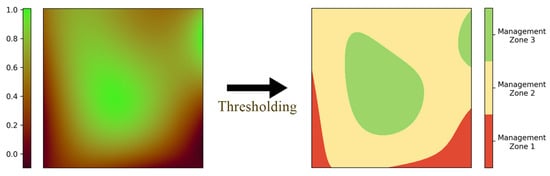
Figure 1.
The process of MZ delineation from a performance function across the field.
Another practice of soil sampling is benchmark sampling. In this practice, the soil is sampled from a benchmark site—which is a very small area within the entire field or within each MZ—rather than making a soil composite [5]. Keyes and Gillund showed that benchmark sampling can replace composite sampling without losing the test precision [8]. The benefit of benchmark sampling is that by sampling from the same benchmark sites over the years, the trend of soil nutrient changes can be tracked [4]. Tracking the changes in soil nutrients has applications in soil monitoring and soil nutrient management. For this method of sampling, it is important to select a small area of the field as a benchmark site that is representative of the soil of the field. Choosing a single benchmark site for the entire field suffers again from the issue of not accounting for soil variability. Instead, using the soil sampling management zone technique, benchmark sampling can be done per MZ, and the result of the test applies to all parts of that MZ. This method of testing not only provides precise information about the soil composition but also reveals the trend of the nutrient changes for each MZ while remaining a cheap method of soil testing.
The main challenge of benchmark sampling is selecting a benchmark site within each MZ that is a proper representative of that MZ. The criteria for the representative area of the MZ depend on the method used for delineating the MZs. In general, several distances, including the distance to boundaries of MZs and the distance to specific values of performance functions, like the median or mean of MZs, are important. Moreover, some non-representative or non-accessible areas usually must be avoided.
The process of selecting benchmark sites based on the criteria is cumbersome, requiring integrating various datasets and manually comparing different values. Therefore, the challenge is how to automatically satisfy all criteria and constraints using the available datasets. The proposed framework offers an automated and algorithmic approach that integrates various data inputs, such as MZs, the digital elevation model, and field boundaries into a multi-objective and multi-constraint optimization model. By solving this optimization model, the framework generates benchmark sites that meet specific needs. In this framework, for each MZ, several distance metrics are calculated and combined into a single-weighted error function. By minimizing this error function, the optimal area for placing benchmark sites is determined. In cases where MZs are not available, any given performance function, typically time-varying remote sensing measurements, can be used instead. MZs can then be determined using a flexible thresholding technique.
The paper proposes an algorithmic framework that effectively automates the process of selecting benchmark sites for a field, based on its georeferenced shape file and remote sensing measurements in time. The framework is highly adaptable and can easily incorporate different measurements and site selection criteria. Compared to the conventional GIS process, which typically takes several days with the involvement of GIS technicians, our automatic process of generating benchmark sites using the proposed algorithmic framework takes only a few seconds. Therefore, the novelty of this work is defining a methodological technique to integrate multiple layers of raster and vector data and making decisions by defining multiple objectives and constraints. The paper also provides a comprehensive evaluation and analysis of the resulting benchmark sites to confirm that our optimization model works as expected. Furthermore, the paper demonstrates how our framework can be leveraged to incorporate different criteria that are not considered in this work, making it a highly adaptable tool for selecting benchmark sites for fields. To summarize, the main objectives of this paper are as follows:
- The primary objective of this work is to provide a framework to automate the process of selecting benchmark sites by avoiding typical manual GIS processes like integrating different layers of information and manually comparing the values of objectives for selected points.
- The framework should be flexible and allow for the integration of new data and defining new objectives and constraints.
2. Background
Recent advances in remote sensing have proven to be useful for agricultural applications at various stages of crop production [6,9]. Various satellite and UAV-attached sensors, such as light detection and ranging (LiDAR), thermal, and multi-spectral sensors have been used to assess the topography, soil moisture, temperature, crop health (vegetation indices), and other useful properties at both farm and larger scales [9]. It may not be feasible to sample every point in a field; we have to determine the soil properties on the non-sampled points based on the available soil samples [10]. Remote sensing helps us to understand the variation in soil and fill in the gaps.
In this section, the previous work and the background knowledge required to understand this paper are discussed. First, we discuss the main methods used for delineating the MZs and the criteria used for selecting benchmark sites in the literature. Then, we introduce the GIS platform used in this work, Discrete Global Grid System, in detail. Finally, the general methods used to solve multi-objective optimization problems are presented.
2.1. Delineation of Management Zones
Management zones play an important role in our method. Therefore, we need to know how they are constructed before discussing how to select the benchmark sites. Different delineation methods for site-specific management zones exist based on different information, usually yield maps, soil properties, topographic properties, electrical conductivity data, or remote sensing and vegetation indices. Hornung et al. [11] have compared the soil-color-based and yield-based methods. Both methods require the availability of agricultural maps, such as soil color and texture maps, yield maps, and topography maps. Fraisse et al. [12] proposed a method that relies on soil electrical conductivity data. However seasonal effects, like weather, have an impact on the electrical conductivity, so the electrical conductivity map of a field cannot be compared to one from another field.
Satellite imagery presents a great added value because of its availability and relatively low cost. Georgi et al. [13] propose an automatic delineation algorithm based on only satellite remote sensing data. In this method, they select satellite images of the field that show the spatial pattern of plant growth. Then, they extract the near-infrared (NIR) band of the selected images and average them over years to form the performance function.
2.2. Benchmark Soil Sampling
Benchmark soil sampling involves taking soil samples from a designated benchmark site, which is a small area within either the entire field or each MZ [4]. Research has shown that benchmark sampling is comparable in accuracy to composite sampling in terms of test precision [8]. The advantage of benchmark sampling is that by consistently sampling from the same benchmark sites over time, changes in soil nutrient trends can be monitored [4]. Due to soil variability, different sampling designs attempt to find representative points of a field with the help of different sensory information (e.g., electrical conductivity of the soil) [14,15]. Another sampling scheme acts in multiple stages, where first, a large number of points are generated and then filtered based on some criteria [16]. One study introduces a method for identifying the representative sampled points from a set of already sampled and tested points using clustering algorithms and calculating fuzzy membership values for each point [17]. Overall, finding representative areas of the field remains a challenge for benchmark sampling. Several studies have suggested that management zone delineation provides a basis for benchmark soil sampling [18,19,20,21,22]. Although MZs are assumed to be homogeneous for management purposes, the soil within each MZ still varies by location. Therefore, it is important to carefully select representative areas rather than making arbitrary choices. Different studies have used approximate measures to manually select representative locations for benchmark sampling [23,24,25]. For example, the benchmark sites in Alberta were selected to be representative of soil landscapes and agricultural land use found in the agricultural area, under the Alberta Environmentally Sustainable Agriculture (AESA) Soil Quality Monitoring Program [23].
Benchmark sampling is a practical and cost-effective method of soil sampling [26,27]. Typically, the benchmark sampling sites are selected by experts after field surveys, or by farmers using some guidelines like in [5]. However, the literature lacks algorithmic methods for selecting benchmark sites from MZs. This paper addresses this gap by introducing an algorithm for the automatic selection of benchmark sites that relies solely on satellite images and does not need any auxiliary data (e.g., electrical conductivity sensors).
2.3. Discrete Global Grid Systems
To support integrating different inputs, calculating various distances (e.g., to the MZ boundaries) efficiently, solving the optimization problem, and automatically repeating this process for various regions, a geographic information system (GIS) is needed. In recent years, discrete global grid systems (DGGSs) have emerged as a promising next-generation of GIS platforms, and are useful for the integration and analysis of remote sensing data [28] as well as congruent geography applications [29].
A DGGS is a multi-resolution discretization of the earth that is used to address different limitations in traditional GISs [29,30,31]. Our automated algorithm leverages some of the benefits of DGGSs. We use a DGGS as a common reference model to integrate the different data needed for selecting the sampling site, including satellite imagery and digital elevation models (DEMs) [32]. A DGGS not only facilitates the analysis by making the data integration transparent but also by providing efficient tools and operations including distance transform [33]. Distance transform is a tool that can be used to efficiently calculate the geodesic distance of all the points of a region to the complex boundary of the MZs. A DGGS naturally discretizes the earth into mostly regular shapes known as cells. Figure 2 depicts this discretization at different resolutions. The specific DGGS implementation that is used in this work is a Disdyakis Triacontahedron DGGS, which is described in [34].
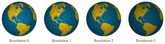
Figure 2.
Disdyakis Triacontahedron DGGS in the first 4 resolutions.
2.4. Solving a Multi-Objective Optimization Problem
A multi-objective optimization problem is not trivial to solve. The preferences of objectives should be given for each specific optimization problem, otherwise, there is no optimal answer to a multi-objective optimization problem. In this case, a set of answers can only be Pareto optimal [35]. A Pareto optimal answer means you cannot make any objective better without making other objectives worse. In general, methods for solving a multi-objective optimization problem can be categorized into three categories: methods with (1) a priori articulation of preferences, (2) posteriori articulation of preferences, and (3) no articulation of preferences [35]. The most common and general method of solving is to combine all objectives into a function to make it a single objective function, which is called scalarization. However, different scalarization methods, such as global criterion, achievement function, compromise function, and objective product, use different combinations [35]. If these methods implement a weighting system for combination, they utilize a method with a priori articulation of preferences.
A weighted scalarization method converts a multi-objective optimization problem into a single-objective optimization problem. The typical method of solving a single-objective optimization problem is solving for critical points directly if the mathematical expression of the objective function is well-known and is differentiable (e.g., linear least squares) [36,37]. When the mathematical expression for the objective function is unknown, gradient-based methods, such as gradient descent, Newton’s method, or the quasi-Newton method, can be used [36,37]. These methods typically start from a random point and rely on the gradient to find the direction of the steepest descent. The gradient is usually approximated by numerical methods for the objective function. This process is iteratively repeated until the algorithm converges. However, these methods may converge to a local minimum depending on the starting point. If the domain of the objective function is discrete and bounded (e.g., raster data such as satellite imagery), a complete search method can be applied by evaluating the objective function for each value in the domain (e.g., each pixel in the raster). This approach guarantees finding the global minimum but can be expensive if the domain is large. A DGGS, as a data integration platform, is a discretization of the earth; hence, it can be naturally used to evaluate and solve an optimization problem efficiently. Moreover, we can control the size of the search space by changing the resolution of the DGGS to tune the trade-off between performance and accuracy.
3. Methodology
The main challenge of benchmark sampling is selecting a benchmark site within each MZ that is a proper representative of that MZ. The aim of this work is to provide a framework for considering multiple requirements and finding the best benchmark sites according to criteria. The criteria for the representative area of the MZ depend on the method used for delineating the MZs. However, we chose a specific MZ delineation method and set of criteria to build, test, and demonstrate our framework. In general, the following criteria are important for a representative benchmark site [38]:
- Being close to the median of the performance function used for MZ delineation within each MZ: The median is statistically considered a good representative of a data set because it is a robust measure describing the central tendency of the data. Therefore, it is desired to select the benchmark site in a place where its performance function value is close to the median of its MZ. Figure 3a shows a visualization for this criterion for only one MZ in which blue regions have a smaller absolute difference to the median.
- Being far from the boundary of the MZ: Areas close to the MZ boundaries are more sensitive to input changes or year-to-year variation. To obtain more robust benchmark sites, it is better to find areas away from the boundaries of each MZ. Figure 3b shows this criterion for one MZ; locations with darker blue are farther from the boundary.
- Being close to the anchor points (e.g., sampled points from previous years): To perform benchmark sampling, if sampled points from previous years (or growing seasons) are available, it may be desirable to select the new benchmark site close to the previously tested points. These optional anchor points can be useful for scenarios in which the trend of soil changes over the years should be analyzed. Also, this criterion can be used if the growers, for any reason, prefer to find a benchmark site near some given anchor points.
- Steepness: The nutrient levels at steep areas may vary a lot from year to year. Moreover, if an area is steep, it may not be accessible for the sampling truck. Therefore, it is desired to select benchmark sites away from steep regions.
- Avoiding headlands: Headlands are areas of the farm field where heavy agricultural machines, such as combine harvesters, take turns. These areas might be affected by denser soil and overlapping application of fertilizer. Hence, these areas are not representative of the entire field and should be avoided.
- Avoiding inaccessible areas: Inaccessible areas should be avoided so that sampling trucks can collect samples.
- Avoiding the proximity of benchmark sites in other MZs: The selected benchmark sites in different MZs should be far away from each other to ensure the benchmark sites do not all come from a small region of the field. Figure 3c shows an example of benchmark sites that are concentrated in a small area versus benchmark sites that are distanced from each other.
In various scenarios, all or a subset of these criteria must be satisfied.
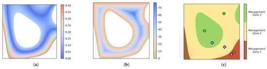
Figure 3.
Criteria for MZ representative area. (a) absolute difference to the median value of the underlying function for MZ 2 (the numbers are in the unit of the performance function); (b) the distance to the boundaries of MZ 2 is shown using a cool–warm color map (in meters); (c) blue diamonds are benchmark sites concentrated in the lower right part of the field, while green circles are benchmark sites that are distanced from each other.
We formulate these criteria as a constrained multi-objective optimization problem. Criteria that specify areas to avoid are our constraints and criteria that we want to optimize for are objectives. One of the most common approaches to a constrained multi-objective optimization problem is the weighted sum method, as follows [35]:
where are objective functions that need to be optimized together and are constraints. F is the global criterion, which is set to be minimized.
The main input data, which are performance function (usually comes from satellite imagery or sensor measurement) and DEM, come in discrete space; hence, objective functions are naturally calculated in discrete space too. Consequently, we need a common discretization of space to store input data, calculate the objective functions, and solve the optimization problem. We exploit the multi-resolution property of a DGGS to choose a resolution as a discrete space.
Our automated process of selecting benchmark sites for a field is presented in Figure 4 in six steps. The process starts by loading the boundary of the field in step 1. In step 2, the performance function and DEM are loaded either by downloading them or loading them from a local cache. Step 3, constructs the MZs from the performance function for step 4. The main contributions of this paper are in steps 4 and 5. In step 4, first, MZs, performance function, and DEM data are resampled into DGGS cells at the target resolution, which means that, for each DGGS cell, we know what the MZ, performance function value, and elevation are. Next, we compute all of the objectives and constraints and store them back in the DGGS cells. All of the objectives are computed on the centroid of DGGS cells. In step 5, the objectives are normalized and combined in a single error function to solve the optimization problem. A complete search in DGGS cells finds the optimum benchmark site. Lastly, in step 6, the selected benchmark sites are saved in a GeoJSON format.
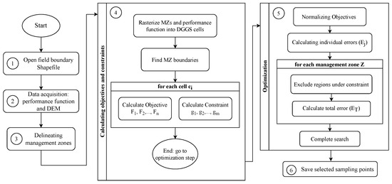
Figure 4.
The flowchart of selecting benchmark sites for a new field.
In Section 3.1, we explain the specific MZ delineation method used in our framework (step 3 of flowchart), and in Section 3.2, we define a set of objectives and constraints and explain how our framework is built to satisfy the objectives and constraints (steps 4 and 5 of flowchart).
3.1. From Data to Management Zones
The performance function is the key to delineating the field to MZs. There are several choices for the performance function. For example, Georgi et al. used the average historical satellite imagery as a performance function [13]. We use a similar method to construct the performance function from the normalized difference vegetation index (NDVI) as an indicator for plant health [38]. Moreover, a recent study shows that both soil electrical conductivity and NDVI are correlated to soil nutrients [39]. This performance function is taken from [38] and is called the fertility index, which is important to this work but is not the novelty of this work. The fertility index serves as a proxy measure to approximate the fertility of the soil by monitoring the historical growth of plants. Higher fertility index values indicate better growing conditions (i.e., soil fertility), as plants have historically grown well in those areas. Similarly, in the final delineated MZs, lower MZs are regions of the field that perform poorly while higher MZs correspond to better-performing regions. We use Sentinel-2 bottom of the atmosphere (BOA) reflectance data obtained from Sentinel-Hub data provider [40] in this delineation process. This delineation process is described in three following steps:
- Selecting images: One image as a good representative for each growing season is selected from the recent years (e.g., 3 to 6 years). The criteria for selecting this image stipulate that it should be both cloud- and haze-free and taken close to the harvest time to optimally showcase the soil’s potential. We use the cloud probability layer (CLP) with a threshold of 5% to ensure cloud-free images. This image represents the variation in soil fertility through the visual growth of plants. Figure 5 presents an example of the selected images for a given field. Note that, although these images are displayed in RGB colors, red, and near-infrared (NIR) bands are used in calculating performance function.
- Calculating the performance function—fertility index (F-index): The normalized difference vegetation index (NDVI) is calculated for each of the selected images using red and NIR bands [41]. While the range of the NDVI is between , for the selected images, the range of values is usually around with the mean around . Then, the NDVI values of each image are normalized and scaled in a way that the mean value M is a fixed number in the range (e.g., ). Finally, the normalized NDVI values are averaged and the resulting averaged normalized values are referred to as F-index (see Figure 6).
- Thresholding: To delineate the F-index into MZs, the next step is to divide the entire range of the F-index into a certain number of bins B (e.g., B = 6). The F-index thresholds are selected in a way that the area of the MZs forms a normal distribution. The resulting map after thresholding is called F-Map (see Figure 6). The number of bins (i.e., MZs) is usually chosen based on the area of the field. However, an arbitrary number of bins can be constructed using this method.
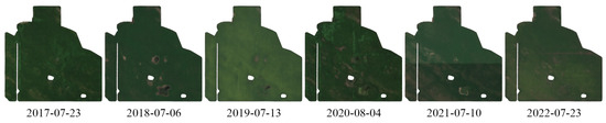
Figure 5.
An example of the selected satellite images for the delineation process.
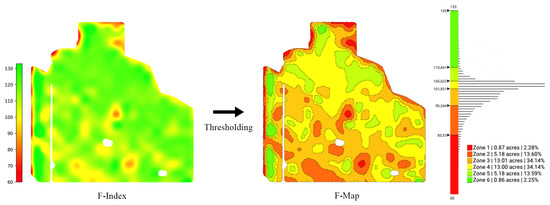
Figure 6.
An example of an F-index, F-Map, the histogram of the F-index, and the associated thresholds.
Figure 6 presents an illustrative example of an F-index and F-Map along with a histogram of the F-index and the thresholds used in the process. The histogram of the F-index (see Figure 6 right) depicts the distribution of the performance function across the field. Upon examining the histogram, we observe that roughly 70% of this field has F-index values between 95 and 105. As a result, dividing the range of F-index values into equal-length bins would yield MZs with a very small area. Likewise, if the field is divided into equal-area MZs, some MZs will have a substantial variation in the F-index, while some other MZs will have a very narrow range of values. To address this issue, the threshold values are selected in a way that the areas of MZs follow a normal distribution.
3.2. Optimization Model
Once we have evaluated MZs (i.e., F-Map), the next question is how to identify the optimal benchmark sites within each MZ. As discussed at the beginning of this section, there are several objectives and some constraints that a site must meet to be considered a good representative point of an MZ. Based on the discussed criteria, we chose the following objectives and constraints in building our framework:
- Objective , close to the value of the median F-index.
- Objective , away from the MZ boundaries.
- Objective , close to the anchor points (optional).
- Objective , belongs to the flatter regions.
- Constraint , avoids certain regions: In practice, it is desired to avoid locating the benchmark sites in certain regions (e.g., inaccessible and unrepresentative areas). Normally, the benchmark site should be at least meters (e.g., 30 m) away from any headlands (headland condition).
- Constraint , avoids the proximity of benchmark sites in other MZs
We formulate these requirements as a constrained multi-objective optimization problem. The objective functions to must be optimized together in consideration of constraints and . The objectives are distance-based and we aim to minimize all of them as best as possible. The two constraints are binary concepts that must be adhered to within the feasible space of site locations. However, some of the objectives can also be considered as constraints. For example, we can maximize the distance to the MZ boundaries as an objective (), or we can set a constraint that the benchmark site must be at least n meters away from any MZ boundary. Although “being away from the boundary with a certain distance” is sufficient, to keep our optimization model flexible and avoid adding another parameter, we consider this property as a distance-based objective. The same thing can be said about the steepness and distance to anchor points. If we set thresholds, we transform our objectives into constraints that exclude any space that does not meet the threshold. However, it is important to note that some of these spaces may still be valuable in terms of other objectives and finding good thresholds to not end up with empty search spaces is difficult.
3.2.1. Computing the Objective Functions
The first step toward solving the optimization problem is calculating the values of objective functions. In this section, we discuss how each of the objective functions to are calculated. The resolution of satellite data (and F-Map) is 10 m (10 m × 10 m square pixels), while the DEM data comes in 12 m resolution. Thus, we use resolution 19 of Disdyakis Triacontahedron DGGS [34], as the target resolution in which DGGS cells (Avg. cell size = 61.8 m2) are a bit smaller than the input data sources. Then, the F-index, F-Map, and DEM data are resampled into DGGS cells at the target resolution. Next, we compute all of the objectives and store them back in the DGGS cells.
- Close to the value of the median F-index (): The first objective is to minimize the distance between the F-index values of the MZ cells and , the median of the management zone Z. Let us denote the DGGS cells of Z by , and their respective F-index values by . This objective is defined as:Figure 7 shows a visualization of this objective function. The blue colors in this visualization show a smaller absolute difference between each cell’s F-index and the median F-index.
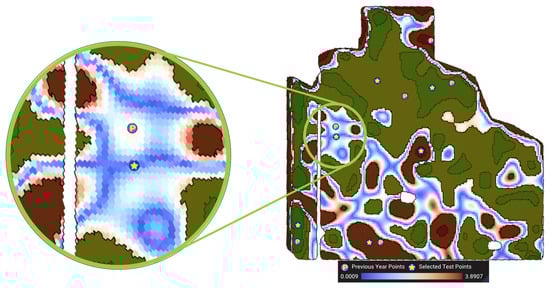
Figure 7.
Visualization of the absolute difference to the median F-index for MZ 3.
- Away from MZ boundaries (): We use the distance transform operator on top of the DGGS [33] to compute the geodesic distance of each cell to S, the spatial boundary of management zone Z. The distance transform efficiently calculates the geodesic distance of all cells in a region to a given vector feature (i.e., the MZ boundaries). The second objective is to maximize this distancewhere denotes the geodesic distance of to S. Figure 8 shows a visualization of this objective function. The cooler the colors (darker blue) the farther the cell is from the boundaries.
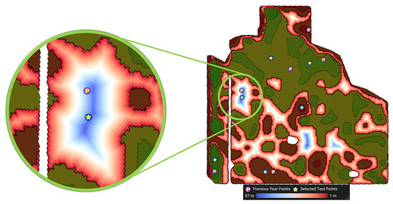
Figure 8.
Visualization of the distance to boundaries of MZ 3. The farthest cell from the boundary is 87 m away from the boundaries.
- Close to anchor points (): Let represent the anchor point for the management zone Z (e.g., the sampled point from previous years). Again, using distance transform [33], we determine the geodesic distance from the anchor point to the centroid of all cells within Z. The third objective, , is to minimize this distancewhere denotes the geodesic distance of to the anchor point . Figure 9 shows a visualization of this objective function. The cooler the colors (darker blue), the closer the cell is to the anchor point.
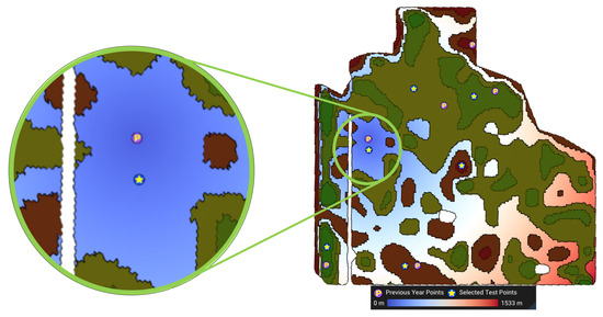
Figure 9.
Visualization of the distance to the anchor point (the previous year’s point) for MZ 3. The farthest cell from this previously sampled point is 1533 m away from it.
- Belongs to flatter regions (): The steepness of the cell (denoted by ) is calculated from the DEM of the field by calculating the gradient vector. The gradient vector shows the direction of change of elevation, which is approximated using the difference in elevation between neighboring cells. Steepness is then determined bywhere is the normal vector of the cell . Figure 10 shows a visualization of this objective function. The cooler (or darker blue) the colors, the flatter the region in which the cell is located.
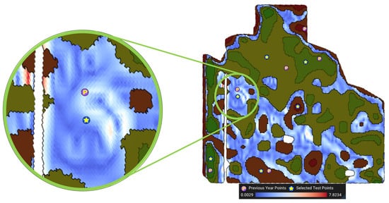
Figure 10.
Visualization of the steepness for MZ 3. The legend shows the steepness in degrees. The steepest point of this MZ is 7.8 degrees steep.
3.2.2. Computing the Constraints
In this section, we discuss how to determine the feasible space of the optimization by calculating constraints for each cell inside the field.
- Avoid Certain Regions () We trivially exclude any cells from the inaccessible and unrepresentative regions by subtracting these regions from the entire field. For the headland condition, we use the distance transform operation of DGGS [33] to calculate a buffer of meters from the boundary of the field to avoid the areas under the headland. Figure 11 shows the areas of the farm avoided due to headland.

Figure 11.
The extracted headland of the farm field ( = 50 m).
- Avoid the Proximity of Benchmark Sites in Other MZs () Our goal is to select benchmark sites that are from a larger region of the field to better represent the entire field. To achieve this, we set a minimum radius between the sites (see Figure 12). This global constraint is unique compared to other criteria that are local to their respective MZs. We begin by selecting a benchmark site in one MZ and then limiting the areas in other MZs that are within the specified radius of this site. We continue this process iteratively until we have chosen benchmark sites for all MZs. To do this, we remove from the search space if for all already selected sites t (see Figure 12).
- By using this method, the benchmark sites selected earlier have an advantage over the ones chosen later, as the latter are subject to more constraints. If the is small, the change of order has a minimal impact. However, for a larger , it makes sense to prioritize MZs according to their level of importance. Therefore, we start with the most important MZ in order to find a more optimal benchmark site for it, and then we continue to select benchmark sites for less important MZs. The most important MZ is the one that best represents the entire field. Hence, the most important MZ is the one with its median F-index closest to that of the entire field. We sort the MZs based on the distance of their median F-index to the median F-index of the entire field. The radius mentioned above can be dynamically changed, but the default is set to be 15% of the field’s diameter. Figure 12 shows how we use this radius to force the selected benchmark sites to be at a reasonable distance from each other.
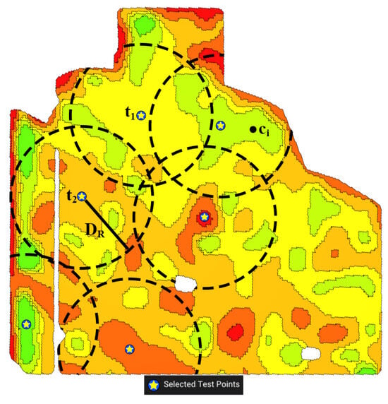
Figure 12.
The enforced distancing between selected benchmark sites. and are the already selected benchmark sites. When deciding on point in the next MZ, we only check the distances to and .
3.2.3. Solving the Optimization Problem
With all objective functions and constraints ready, we need to optimize them together. To satisfy constraint , we solve the optimization for each MZ separately in the order of importance discussed in Section 3.2.2. For each MZ, to accommodate the constraints, we remove DGGS cells under constraint from our feasible search space. This not only ensures that no point under constraint will ever be selected as a benchmark site but also makes the optimization more efficient by reducing the search space. Next, to solve the multi-objective optimization problem we use a scalarization method which is a common method that transforms a multi-objective optimization problem into a single-objective optimization problem [35]. Because we have calculated all of our objectives and constraints in the discrete space of a DGGS (resolution 19 of Disdyakis Triacontahedron DGGS. Avg. cell size = 61.8 m2 [34]), for a 200-hectare field, the total unconstrained search space will have roughly 32,400 cells. This is a very small search space and modern personal computers can evaluate the objective functions for the entire space within a fraction of a second. Hence, to efficiently find the global minimum of the objective function, we perform an efficient complete search on the feasible search space (i.e., comparing objective functions on ). The tractability of the search space is the result of using DGGSs for discretization and data integration. The size of the search space is controllable by utilizing the hierarchy of the DGGS.
To transform our multi-objective optimization problem into a single-objective optimization with a scalarization method, we use a weighted squared sum method. A weighted squared sum enables us to control the effect of each objective function relative to each other and also to penalize large errors. With this, we combine all of the objectives into a global objective function or an error function. Before combining, we first normalize all the individual objective functions. Without normalization, objectives with large values may overpower and dominate the optimization process. To map the objective function into the range , we use a simple linear mapping:
Next, we define an error function for each of the objectives, as follows:
Now, we have a vector of error functions. In order to scalarize these errors into a single error function, we combine them using the weighted sum of squares:
where is the weight of objective , and m is the number of objectives ( in our case). Figure 13 shows the visualization of the error function and the yellow star is the location of the minimum of this function. For illustrative purposes, the constraints are not removed from the search space in this figure.
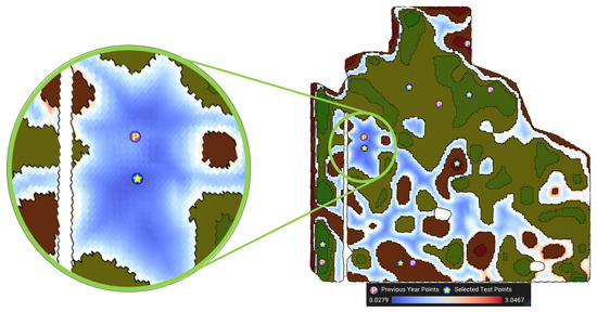
Figure 13.
Visualization of the error function for MZ 3. All weights are set to 1 (, ) in this figure. at the optimal point (denoted by the star) is 0.0279.
Figure 14 shows the final error function only for feasible search space considering constraints for all MZs. The order of the MZ optimization in this figure is MZ 4, MZ 3, MZ 5, MZ 2, MZ 6, and lastly MZ 1. The areas under the headland constraint () and distribution constraint () are marked in pink.
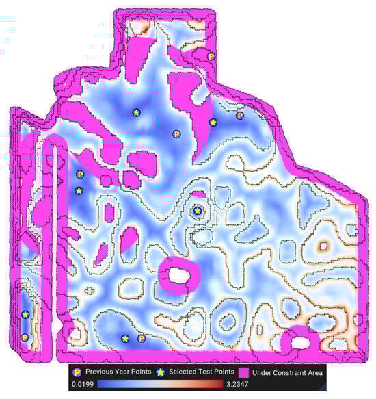
Figure 14.
Visualization of the final error function for the entire field. All weights are set to 1 in this figure.
4. Results and Evaluation
The method is implemented in C++ programming language and uses OpenGL for rendering the graphical interface. The application provides two interfaces: a graphical user interface (GUI) for illustration and debugging purposes and a command line interface (CLI) to fully automate the process. The CLI version only takes a few seconds for a relatively large field (see Table 1) and only needs the boundary of the field as input with a few additional settings. In comparison, using the more traditional method, a GIS technician must go through works such as drawing the field polygon, downloading the satellite imagery, finding MZs, and many interactive measurements using GIS software to determine benchmark sites. The interactive measurements include visually finding some candidate points per MZ and calculating the values for each criterion (e.g., what is the distance of the given point to the MZ boundaries? How close is the point’s performance to the median?) to compare the candidate points. Not only this entire process using the traditional method would take multiple days, but also in the end, this is only a rough approximation of the desired sample points as it only uses some candidate points picked by the GIS technician. Our introduced framework (steps 4 and 5 in Figure 4) is necessary to entirely avoid this manual process. To demonstrate the repeatability of this automatic approach, and to show that our algorithm works for different fields, we chose five different fields of varying sizes across the Canadian provinces of Alberta, Saskatchewan, and Manitoba. The list of the fields and the execution time of our algorithm is given in Table 1.

Table 1.
The list of fields used for evaluation. The total execution time captures the entire process, including loading data from the local cache (tested on a computer with an Intel Core i7-6700 CPU).
Figure 15 shows the selected benchmark sites for each field. To generate these results, six years of satellite imagery (2017–2022) is used for MZ delineation, the headland () is set to 30 m, the for each field is given in Table 1, and the objective weights are all set to 1. The effect of different weights on optimization is discussed later in the next subsection. To demonstrate the correctness of the optimization, we calculated the statistics of the objectives for each MZ for all fields. The statistics for field 1 are reported in Table 2 and the same statistics for other fields are presented in Appendix A. Each row of these tables includes the mean and the range of each objective across the MZ along with the best value for that objective, the objective value at the selected benchmark site, and the percentage improvement relative to the mean ().
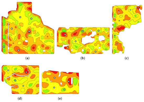
Figure 15.
Selected benchmark sites for the field (a) 1, (b) 2, (c) 3, (d) 4, and (e) 5. Yellow stars represent selected test points.
Table 2.
The range and average of the objectives are compared to the objectives of the selected benchmark sites for field 1.
The alternative to benchmark sampling in the MZs is MZ composite sampling. If composite sampling is done properly, the objectives of the composite sample should be close to the mean of the objectives of the MZ. Hence, by reporting these statistics in Table 2 we show that the objectives of the selected benchmark sites are improved in comparison to the composite sampling. This enables the farm manager to track the nutrient changes. In all the fields we evaluated, the objective for the selected benchmark site is always better than the mean of all the cells of the MZ except for a couple of cases in fields 1 and 3 that are slightly worse. In both these cases, the problematic benchmark sites are in the first and last MZs, which represent the smallest area of the field (see Figure 6). Selecting good benchmark sites for the middle MZs—which represent the majority of the area of the field—at the cost of slightly worse than mean benchmark sites for the first and last zones is reasonable. The presented statistics show that in the middle MZs (i.e., MZs 3 and 4 out of the six total), the objectives at the benchmark sites are significantly better than the mean.
Overall, our algorithm produces better benchmark sites than a composite sample according to our criteria. Objective (being close to the anchor points) is excluded from our objectives because we did not have anchor points for any of the fields. Moreover, we excluded cells under constraint from our mean and range calculations to obtain a fair comparison. Lastly, our optimization constraints and are satisfied; no benchmark sites are selected in headland () or in proximity () to other benchmark sites. Constraint , in combination with objective , will result in a relatively good covering of the field by benchmark sites which can be visually verified by looking at Figure 15.
To comprehensively summarize these tables, for each field, we report the mean percentage improvement over all MZs of the field. The mean percentage improvement is reported in Table 3 for each objective. This aggregated result emphasizes how the representative site objectives are improved when compared to composite sampling.
Table 3.
The mean percentage improvements of the selected benchmark sites.
4.1. Modularity and Extendability
One significant advantage of our framework is its modularity and extendability. Although we chose a specific performance function, a specific MZ delineation method, and a specific set of criteria to demonstrate our optimization model, our algorithmic framework is flexible and defines a mathematical structure to be used in other scenarios as well. The data integration in our framework is handled using a DGGS which allows additional datasets such as different satellite imagery (e.g., thermal imagery or radar data), aerial imagery, and wetland maps, to be integrated with the algorithm in the future as needed.
For example, our framework obtains an MZ map as input which can be constructed from any performance function. Apparent soil electrical conductivity (EC) is a particular performance function that is proven to highly correlate with soil nutrients and is useful for MZ delineation [39,42]. To demonstrate that our framework works for other performance functions as well, we used a real EC dataset for a field in Selbitz (Elbe), Germany [43]. For simplicity, we used the same thresholding method to delineate MZs from EC data. The left column in Figure 16 shows the EC data and the F-index for this field in Germany and the right column is the selected benchmark sites along with the delineated MZs. This figure demonstrates that our framework is general and works for an arbitrary performance function.
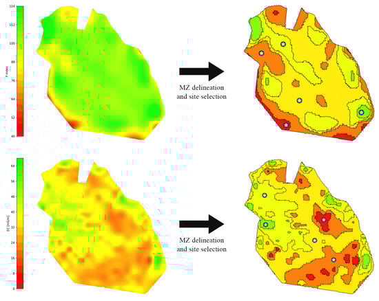
Figure 16.
Using the apparent soil electrical conductivity map as a performance function. Yellow stars represent selected test points.
Similar to the performance function and MZs, the representative site criteria can be extended in both forms of objectives and constraints. For example, new constraints to avoid power lines, pipelines, and other barriers are just other regions to avoid, much in the same way as the headland in . Additionally, more objectives can be added or the existing objectives can be swapped with another one. For example, instead of , one may want to use the first quantile and third quantile along with the median. In this case, one can easily swap the to another objective, which calculates the difference of the F-index to another value (e.g., the first or third quantile or mean). Figure 17 demonstrates the application of the first and third quantiles along with the median (second quantile) as a new objective, which shows that our framework can be used to satisfy new criteria.
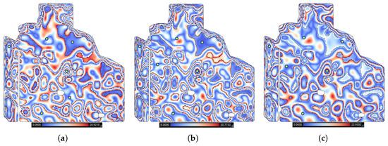
Figure 17.
A visualization of the difference of the F-index of each cell with (a) first quantile, (b) second quantile (median), and (c) third quantile of the F-index of each MZ. Yellow stars represent selected test points.
4.2. Discussion
Our automatic benchmark site selection method is flexible in various aspects. Specifically, the relative importance of the objectives and the number of MZs are tunable. The following subsections discuss and demonstrate each of these flexibilities of our method.
4.2.1. Optimization Weights
One flexibility of our method is defining the importance of objectives relative to each other by means of weights. The weights are available as a simple interface for the end user to adjust if necessary. For example, if a field is very flat, assigning a lower weight for steepness can help the algorithm to optimize better for other criteria. Looking at Table 4, we observe that a lower weight for steepness helped the model lower the difference to the median F-index by 1.124 units. Recalculating the error after changing the weights is instant, which means that the user can quickly and efficiently test different configurations to obtain the desired results.
Table 4.
The effect of weights on objectives. This table is based on MZ 2 on field 1.
4.2.2. Number of MZs
The number of MZs is usually set based on the area of the field. However, our automated method is adjustable and can delineate a field to any number of MZs. For example, if one wants to account for within-zone heterogeneity, one can divide each MZ into multiple MZs, and the algorithm finds a test point for each refined MZ. This is practical when a deep understanding of the variability of the soil of a field is needed. Figure 18 shows an example of a varying number of MZs on a field. Table 5 demonstrates that our method remains fast and performant when the number of MZs increases. We intentionally decreased the for the higher number of MZs because more benchmark sites have to be fit in the same area. Moreover, for the results presented in Table 5, the is set to 0, because in the higher number of MZs, the lower MZ ends up completely in the headland. In practice, the MZs with very tiny areas are not worth sampling.
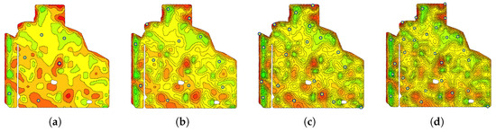
Figure 18.
Delineating a field into (a) 6, (b) 12, (c) 20, and (d) 30 MZs results in the same number of the selected benchmark sites. Yellow stars represent selected test points.
Table 5.
The mean percentage improvement for field 1 when the number of MZs varies between 6 and 30 MZs.
5. Conclusions and Future Work
In this paper, we introduce an automated framework to solve the constrained multi-objective optimization problem of selecting benchmark sites. To demonstrate our framework, the optimization includes four different objectives: close to the value of the median F-index, away from MZ boundaries, close to anchor points, and belonging to flatter regions. Two constraints, avoiding certain regions and avoiding the proximity of benchmark sites in other MZs, are also included in the optimization. We showed that this optimization problem can be efficiently solved on a DGGS and the produced benchmark sites are better than an MZ composite sample. The repeatability of the method is shown by testing the algorithms on five different fields. This algorithm takes between 9 and 23 s for tested fields in comparison to a manual process by a GIS technician, which takes days. We discussed the generality and flexibility of our method.
Our framework allows additional datasets, such as different satellite imagery (e.g., thermal imagery or radar data), aerial imagery, and wetland maps, to be used within our algorithm. We showed that different performance functions, including EC and different delineation methods, can be used within our framework. This enables our framework to be suitable for many applications where the MZs are used for soil monitoring, nutrient leaching, and greenhouse gas emissions. However, the usage of this framework in other applications is not explored in this paper and constitutes an area for future research.
Moreover, for future research, it is advisable to apply this method in an environment where there is access to a comprehensive dataset, including a wide range of soil characteristics resulting from dense grid sampling. This approach will facilitate a thorough evaluation of how well the algorithm identifies the representative areas of management zones when compared to each soil parameter. Ultimately, this will lead to a more precise assessment of how well they truly represent those zones.
Author Contributions
Conceptualization, M.K. and F.F.S.; methodology, M.K. and F.F.S.; software, M.K.; validation, M.K. and F.F.S.; formal analysis, M.K. and F.F.S.; investigation, M.K.; resources, F.F.S.; data curation, M.K.; writing—original draft preparation, M.K.; writing—review and editing, M.K. and F.F.S.; visualization, M.K.; supervision, F.F.S.; project administration, F.F.S.; funding acquisition, F.F.S. All authors have read and agreed to the published version of the manuscript.
Funding
This research was supported by the Mitacs Accelerate program and the Natural Sciences and Engineering Research Council (NSERC) of Canada.
Institutional Review Board Statement
Not applicable.
Informed Consent Statement
Not applicable.
Data Availability Statement
No new data were created or analyzed in this study. Data sharing is not applicable to this article.
Acknowledgments
Thanks go out to all members of the GIV research team at the University of Calgary for the insights and discussions. Special thanks go out to Benjamin Ulmer for proofreading the manuscript and providing grammatical suggestions. Special thanks go out to Vincent Yeow Chieh Pang, Garret Duffy, and Jessika Töyrä for the great discussions and insights during the Mitacs project.
Conflicts of Interest
The authors declare no conflict of interest.
Abbreviations
The following abbreviations are used in this manuscript:
| MZ | management zone |
| NIR | near-infrared |
| NDVI | normalized difference vegetation index |
| DGGS | discrete global grid system |
| GIS | geographic information system |
| AESA | Alberta Environmentally Sustainable Agriculture |
| UAV | unmanned areal vehicle |
| LiDAR | light detection and ranging |
| DEM | digital elevation model |
| GUI | graphical user interface |
| CLI | command-line interface |
| EC | electrical conductivity |
| BOA | bottom of the atmosphere |
Appendix A
Table A1.
The range and average of the objectives are compared to the objectives of selected benchmark sites for field 2.
Table A1.
The range and average of the objectives are compared to the objectives of selected benchmark sites for field 2.
| MZ | Objective | Benchmark Site | Mean of All Cells | Percentage Improvement | Best | Range |
|---|---|---|---|---|---|---|
| 1 | Median F-index | 13.393 | 18.202 | 26.4% | 0.000 | [0.000, 47.910] |
| Distance To Boundary | 27.535 | 16.483 | 67.0% | 48.759 | [1.263, 48.759] | |
| Steepness | 2.207 | 2.843 | 22.4% | 1.395 | [1.395, 4.932] | |
| 2 | Median F-index | 2.920 | 4.453 | 34.4% | 0.017 | [0.017, 18.161] |
| Distance To Boundary | 40.850 | 9.775 | 317.9% | 43.235 | [1.263, 43.235] | |
| Steepness | 1.010 | 3.405 | 70.3% | 0.021 | [0.021, 10.844] | |
| 3 | Median F-index | 0.013 | 1.550 | 99.2% | 0.000 | [0.000, 4.431] |
| Distance To Boundary | 56.517 | 12.870 | 339.1% | 56.517 | [1.259, 56.517] | |
| Steepness | 1.046 | 2.700 | 61.3% | 0.006 | [0.006, 11.680] | |
| 4 | Median F-index | 0.140 | 1.075 | 87.0% | 0.000 | [0.000, 2.610] |
| Distance To Boundary | 55.644 | 12.011 | 363.3% | 59.418 | [1.259, 59.418] | |
| Steepness | 1.173 | 2.040 | 42.5% | 0.003 | [0.003, 9.167] | |
| 5 | Median F-index | 0.720 | 1.000 | 28.0% | 0.002 | [0.002, 2.917] |
| Distance To Boundary | 29.709 | 10.057 | 195.4% | 41.810 | [1.259, 41.810] | |
| Steepness | 1.863 | 2.226 | 16.3% | 0.013 | [0.013, 10.052] | |
| 6 | Median F-index | 3.272 | 3.351 | 2.4% | 0.000 | [0.000, 13.995] |
| Distance To Boundary | 23.627 | 9.387 | 151.7% | 33.618 | [1.259, 33.618] | |
| Steepness | 2.146 | 3.095 | 30.7% | 0.108 | [0.108, 8.438] |
Table A2.
The range and average of the objectives are compared to those of the selected benchmark sites for field 3.
Table A2.
The range and average of the objectives are compared to those of the selected benchmark sites for field 3.
| MZ | Objective | Benchmark Site | Mean of All Cells | Percentage Improvement | Best | Range |
|---|---|---|---|---|---|---|
| 1 | Median F-index | 4.590 | 2.883 | −59.2% | 0.126 | [0.126, 8.487] |
| Distance To Boundary | 23.519 | 11.948 | 96.8% | 27.191 | [1.298, 27.191] | |
| Steepness | 2.163 | 3.028 | 28.6% | 0.260 | [0.260, 6.357] | |
| 2 | Median F-index | 0.681 | 2.145 | 68.3% | 0.000 | [0.000, 6.899] |
| Distance To Boundary | 44.390 | 18.374 | 141.6% | 60.355 | [1.291, 60.355] | |
| Steepness | 0.868 | 2.521 | 65.6% | 0.031 | [0.031, 8.747] | |
| 3 | Median F-index | 0.268 | 1.939 | 86.2% | 0.000 | [0.000, 4.174] |
| Distance To Boundary | 86.394 | 18.537 | 366.1% | 91.327 | [1.291, 91.327] | |
| Steepness | 1.759 | 2.137 | 17.7% | 0.026 | [0.026, 9.368] | |
| 4 | Median F-index | 0.344 | 1.834 | 81.2% | 0.000 | [0.000, 5.624] |
| Distance To Boundary | 48.860 | 13.752 | 255.3% | 53.131 | [1.291, 53.131] | |
| Steepness | 1.863 | 2.167 | 14.0% | 0.002 | [0.002, 9.731] | |
| 5 | Median F-index | 0.144 | 1.805 | 92.0% | 0.022 | [0.022, 3.604] |
| Distance To Boundary | 17.555 | 6.031 | 191.1% | 18.800 | [1.295, 18.800] | |
| Steepness | 1.158 | 2.205 | 47.5% | 0.849 | [0.849, 4.675] |
Table A3.
The range and average of the objectives are compared to the objectives of the selected benchmark sites for field 4.
Table A3.
The range and average of the objectives are compared to the objectives of the selected benchmark sites for field 4.
| MZ | Objective | Benchmark Site | Mean of All Cells | Percentage Improvement | Best | Range |
|---|---|---|---|---|---|---|
| 1 | Median F-index | 1.450 | 1.861 | 22.1% | 0.000 | [0.000, 4.030] |
| Distance To Boundary | 24.923 | 11.987 | 107.9% | 34.016 | [1.305, 34.016] | |
| Steepness | 0.917 | 1.132 | 19.0% | 0.115 | [0.115, 2.264] | |
| 2 | Median F-index | 1.341 | 1.829 | 26.7% | 0.019 | [0.019, 6.067] |
| Distance To Boundary | 34.657 | 11.745 | 195.1% | 53.336 | [1.302, 53.336] | |
| Steepness | 0.163 | 1.116 | 85.4% | 0.023 | [0.023, 3.109] | |
| 3 | Median F-index | 0.149 | 1.326 | 88.8% | 0.000 | [0.000, 3.028] |
| Distance To Boundary | 44.455 | 12.907 | 244.4% | 49.212 | [1.298, 49.212] | |
| Steepness | 0.280 | 1.125 | 75.1% | 0.018 | [0.018, 3.517] | |
| 4 | Median F-index | 0.003 | 1.398 | 99.8% | 0.003 | [0.003, 4.184] |
| Distance To Boundary | 30.103 | 9.557 | 215.0% | 34.657 | [1.302, 34.657] | |
| Steepness | 0.737 | 1.093 | 32.6% | 0.014 | [0.014, 3.374] | |
| 5 | Median F-index | 0.034 | 0.626 | 94.6% | 0.034 | [0.034, 1.158] |
| Distance To Boundary | 15.860 | 5.758 | 175.5% | 18.325 | [1.302, 18.325] | |
| Steepness | 0.318 | 0.899 | 64.7% | 0.043 | [0.043, 2.574] |
Table A4.
The range and average of the objectives are compared to the objectives of the selected benchmark sites for field 5.
Table A4.
The range and average of the objectives are compared to the objectives of the selected benchmark sites for field 5.
| MZ | Objective | Benchmark Site | Mean of All Cells | Percentage Improvement | Best | Range |
|---|---|---|---|---|---|---|
| 1 | Median F-index | 2.340 | 5.078 | 53.9% | 0.294 | [0.294, 14.785] |
| Distance To Boundary | 18.382 | 10.907 | 68.5% | 32.534 | [1.216, 32.534] | |
| Steepness | 0.451 | 0.665 | 32.3% | 0.029 | [0.029, 1.712] | |
| 2 | Median F-index | 2.361 | 2.469 | 4.4% | 0.000 | [0.000, 10.209] |
| Distance To Boundary | 85.619 | 22.106 | 287.3% | 87.502 | [1.216, 87.502] | |
| Steepness | 0.510 | 0.934 | 45.4% | 0.010 | [0.010, 4.003] | |
| 3 | Median F-index | 0.168 | 1.441 | 88.4% | 0.000 | [0.000, 3.680] |
| Distance To Boundary | 105.288 | 26.053 | 304.1% | 109.590 | [1.212, 109.590] | |
| Steepness | 0.347 | 0.857 | 59.5% | 0.004 | [0.004, 3.446] | |
| 4 | Median F-index | 0.101 | 3.439 | 97.1% | 0.000 | [0.000, 16.610] |
| Distance To Boundary | 27.363 | 13.264 | 106.3% | 44.053 | [1.216, 44.053] | |
| Steepness | 0.861 | 1.045 | 17.7% | 0.050 | [0.050, 3.369] |
References
- Lavanya, G.; Rani, C.; Ganeshkumar, P. An automated low cost IoT based Fertilizer Intimation System for smart agriculture. Sustain. Comput. Inform. Syst. 2020, 28, 100300. [Google Scholar] [CrossRef]
- Schimmelpfennig, D. Farm Profits and Adoption of Precision Agriculture; Technical Report 1477-2016-121190; United States Department of Agriculture (USDA): Washington, DC, USA, 2016. [CrossRef]
- Harou, A.P.; Madajewicz, M.; Michelson, H.; Palm, C.A.; Amuri, N.; Magomba, C.; Semoka, J.M.; Tschirhart, K.; Weil, R. The joint effects of information and financing constraints on technology adoption: Evidence from a field experiment in rural Tanzania. J. Dev. Econ. 2022, 155, 102707. [Google Scholar] [CrossRef]
- Carter, M.R.; Gregorich, E.G. (Eds.) Soil Sampling and Methods of Analysis; CRC Press: Boca Raton, FL, USA, 2007. [Google Scholar]
- Alberta Agriculture and Food. Nutrient Management Planning Guide; Alberta Agriculture and Food: Edmonton, AB, Canada, 2015. [Google Scholar]
- Mulla, D.J. Twenty five years of remote sensing in precision agriculture: Key advances and remaining knowledge gaps. Biosyst. Eng. 2013, 114, 358–371. [Google Scholar] [CrossRef]
- Pierce, F.J.; Nowak, P. Aspects of Precision Agriculture. In Advances in Agronomy; Sparks, D.L., Ed.; Academic Press: Cambridge, MA, USA, 1999; Volume 67, pp. 1–85. [Google Scholar] [CrossRef]
- Keyes, D.; Gillund, G. Benchmark sampling of agricultural fields. In Proceedings of the Soils and Crops Workshop, Saskatoon, SK, Canada, 16 March 2021. [Google Scholar]
- Khanal, S.; KC, K.; Fulton, J.P.; Shearer, S.; Ozkan, E. Remote Sensing in Agriculture—Accomplishments, Limitations, and Opportunities. Remote Sens. 2020, 12, 3783. [Google Scholar] [CrossRef]
- Radočaj, D.; Jurišić, M.; Gašparović, M. The Role of Remote Sensing Data and Methods in a Modern Approach to Fertilization in Precision Agriculture. Remote Sens. 2022, 14, 778. [Google Scholar] [CrossRef]
- Hornung, A.; Khosla, R.; Reich, R.; Inman, D.; Westfall, D. Comparison of site-specific management zones: Soil-color-based and yield-based. Agron. J. 2006, 98, 407–415. [Google Scholar] [CrossRef]
- Fraisse, C.; Sudduth, K.; Kitchen, N. Delineation of site-specific management zones by unsupervised classification of topographic attributes and soil electrical conductivity. Trans. ASAE 2001, 44, 155. [Google Scholar] [CrossRef]
- Georgi, C.; Spengler, D.; Itzerott, S.; Kleinschmit, B. Automatic delineation algorithm for site-specific management zones based on satellite remote sensing data. Precis. Agric. 2018, 19, 684–707. [Google Scholar] [CrossRef]
- Tarr, A.B.; Moore, K.J.; Dixon, P.M.; Burras, C.L.; Wiedenhoeft, M.H. Use of Soil Electroconductivity in a Multistage Soil-Sampling Scheme. Crop Manag. 2003, 2, 1–9. [Google Scholar] [CrossRef]
- Yao, R.; Yang, J.; Zhao, X.; Chen, X.; Han, J.; Li, X.; Liu, M.; Shao, H. A new soil sampling design in coastal saline region using EM38 and VQT method. Clean–Soil Air Water 2012, 40, 972–979. [Google Scholar] [CrossRef]
- Stumpf, F.; Schmidt, K.; Behrens, T.; Schönbrodt-Stitt, S.; Buzzo, G.; Dumperth, C.; Wadoux, A.; Xiang, W.; Scholten, T. Incorporating limited field operability and legacy soil samples in a hypercube sampling design for digital soil mapping. J. Plant Nutr. Soil Sci. 2016, 179, 499–509. [Google Scholar] [CrossRef]
- An, Y.; Yang, L.; Zhu, A.X.; Qin, C.; Shi, J. Identification of representative samples from existing samples for digital soil mapping. Geoderma 2018, 311, 109–119. [Google Scholar] [CrossRef]
- Chabala, L.M.; Mulolwa, A.; Lungu, O. Landform classification for digital soil mapping in the Chongwe-Rufunsa area, Zambia. Agric. For. Fish 2013, 2, 156–160. [Google Scholar] [CrossRef]
- Fridgen, J.J.; Kitchen, N.R.; Sudduth, K.A.; Drummond, S.T.; Wiebold, W.J.; Fraisse, C.W. Management zone analyst (MZA) software for subfield management zone delineation. Agron. J. 2004, 96, 100–108. [Google Scholar]
- Kozar, B.J. Predicting Soil Water Distribution Using Topographic Models within Four Montana Farm Fields. Ph.D. Thesis, Montana State University-Bozeman, College of Agriculture, Bozeman, MT, USA, 2002. [Google Scholar]
- MacMillan, R. A protocol for preparing digital elevation (DEM) data for input and analysis using the landform segmentation model (LSM) programs. In Soil Variability Analysis to Enhance Crop Production (SVAECP) Project; LandMapper Environmental Solutions: Edmonton, AB, Canada, 2000. [Google Scholar]
- Milics, G.; Kauser, J.; Kovacs, A. Profit Maximization in Soybean (Glycine max (L.) Merr.) Using Variable Rate Technology (VRT) in the Sárrét Region, Hungary; Agri-Tech Economics Papers 296767; Harper Adams University, Land, Farm & Agribusiness Management Department: Newport, UK, 2019. [Google Scholar] [CrossRef]
- Cathcart, J.; Cannon, K.; Heinz, J. Selection and establishment of Alberta agricultural soil quality benchmark sites. Can. J. Soil Sci. 2008, 88, 399–408. [Google Scholar] [CrossRef]
- Card, S. Evaluation of Two Field Methods to Estimate Soil Organic Matter in Alberta Soils; AESA Soil Quality Monitoring Program: AB, Canada, 2004. [Google Scholar]
- Ines, R.L.; Tuazon, J.P.B.; Daag, M.N. Utilization of Small Farm Reservoir (SFR) for Upland Agriculture of Bataan, Philippines. Int. J. Appl. Agric. Sci. 2018, 4, 1–6. [Google Scholar] [CrossRef]
- Nutrien Ag Solutions. Soil Sampling Tips. 2019. Available online: https://www.nutrienagsolutions.ca/about/news/soil-sampling-tips (accessed on 1 May 2023).
- Canola Council of Canada. How to Take a Good Soil Sample. 2013. Available online: https://www.canolacouncil.org/canola-watch/2013/10/02/how-to-take-a-good-soil-sample/ (accessed on 1 May 2023).
- Bash, E.A.; Wecker, L.; Rahman, M.M.; Dow, C.F.; McDermid, G.; Samavati, F.F.; Whitehead, K.; Moorman, B.J.; Medrzycka, D.; Copland, L. A Multi-Resolution Approach to Point Cloud Registration without Control Points. Remote Sens. 2023, 15, 1161. [Google Scholar] [CrossRef]
- Goodchild, M.F. Reimagining the history of GIS. Ann. GIS 2018, 24, 1–8. [Google Scholar] [CrossRef]
- Mahdavi-Amiri, A.; Alderson, T.; Samavati, F. A survey of digital earth. Comput. Graph. 2015, 53, 95–117. [Google Scholar] [CrossRef]
- Alderson, T.; Purss, M.; Du, X.; Mahdavi-Amiri, A.; Samavati, F. Digital earth platforms. In Manual of Digital Earth; Springer: Singapore, 2020; pp. 25–54. [Google Scholar]
- Mahdavi Amiri, A.; Alderson, T.; Samavati, F. Geospatial Data Organization Methods with Emphasis on Aperture-3 Hexagonal Discrete Global Grid Systems. Cartogr. Int. J. Geogr. Inf. Geovis. 2019, 54, 30–50. [Google Scholar] [CrossRef]
- Kazemi, M.; Wecker, L.; Samavati, F. Efficient Calculation of Distance Transform on Discrete Global Grid Systems. ISPRS Int. J. Geo-Inf. 2022, 11, 322. [Google Scholar] [CrossRef]
- Hall, J.; Wecker, L.; Ulmer, B.; Samavati, F. Disdyakis Triacontahedron DGGS. ISPRS Int. J. Geo-Inf. 2020, 9, 315. [Google Scholar] [CrossRef]
- Marler, R.T.; Arora, J.S. Survey of multi-objective optimization methods for engineering. Struct. Multidiscip. Optim. 2004, 26, 369–395. [Google Scholar] [CrossRef]
- Everitt, B. Introduction to Optimization Methods and Their Application in Statistics; Springer: Dordrecht, The Netherlands, 2012. [Google Scholar]
- Wright, J.N.S.J. Numerical Optimization; Springer Series in Operations Research and Financial Engineering; Springer: New York, NY, USA, 2006. [Google Scholar] [CrossRef]
- Schmaltz, T.; Melnitchouk, A. Variable Zone Crop-Specific Inputs Prescription Method and Systems Therefor. Canada Patent CA 2663917, 30 December 2014. [Google Scholar]
- Mazur, P.; Gozdowski, D.; Wójcik-Gront, E. Soil Electrical Conductivity and Satellite-Derived Vegetation Indices for Evaluation of Phosphorus, Potassium and Magnesium Content, pH, and Delineation of Within-Field Management Zones. Agriculture 2022, 12, 883. [Google Scholar] [CrossRef]
- Sinergise Ltd. Sentinel Hub. 2023. Available online: https://www.sentinel-hub.com (accessed on 3 October 2023).
- Pettorelli, N. The Normalized Difference Vegetation Index; Oxford University Press: Oxford, UK, 2013. [Google Scholar]
- Serrano, J.; Shahidian, S.; Marques da Silva, J.; Paixão, L.; Moral, F.; Carmona-Cabezas, R.; Garcia, S.; Palha, J.; Noéme, J. Mapping Management Zones Based on Soil Apparent Electrical Conductivity and Remote Sensing for Implementation of Variable Rate Irrigation—Case Study of Corn under a Center Pivot. Water 2020, 12, 3427. [Google Scholar] [CrossRef]
- Pohle, M.; Werban, U. Near surface geophysical data (Electromagnetic Induction—EMI, Gamma-ray spectrometry), August 2017), Selbitz (Elbe), Germany, 2019. Supplement to: Rentschler, Tobias; Werban, Ulrike; Ahner, Mario; Behrens, Thorsten; Gries, Phillipp; Scholten, Thomas; Teuber, Sandra; Schmidt, Karsten (2020): 3D mapping of soil organic carbon content and soil moisture with multiple geophysical sensors and machine learning. Vadose Zone J. 2019, 19. [Google Scholar] [CrossRef]


Disclaimer/Publisher’s Note: The statements, opinions and data contained in all publications are solely those of the individual author(s) and contributor(s) and not of MDPI and/or the editor(s). MDPI and/or the editor(s) disclaim responsibility for any injury to people or property resulting from any ideas, methods, instructions or products referred to in the content. |
© 2023 by the authors. Licensee MDPI, Basel, Switzerland. This article is an open access article distributed under the terms and conditions of the Creative Commons Attribution (CC BY) license (https://creativecommons.org/licenses/by/4.0/).