Real-Time Parametric Path Planning Algorithm for Agricultural Machinery Kinematics Model Based on Particle Swarm Optimization

Abstract

In order to meet the obstacle avoidance requirements of unmanned agricultural machinery in operation, it is necessary to plan a path to avoid obstacles in real time after obstacles are detected. However, the traditional path planning algorithm does not consider kinematic constraints, which makes it difficult to realize the plan, thus affecting the performance of the path tracking controller. In this paper, a real-time path planning algorithm based on particle swarm optimization for an agricultural machinery parametric kinematic model is proposed. The algorithm considers the agricultural machinery kinematic model, defines the path satisfying the kinematic model through a parametric equation, and solves the initial path through the analytic method. Then, considering the constraints of obstacles, acceleration, and turning angle, two objective functions are proposed. The particle swarm optimization algorithm is used to search the path near the initial path which satisfies the obstacle avoidance condition and has a better objective function value. In addition, the influence of the algorithm parameters on the running time is analyzed, and the method of compensating the radius of the obstacle is proposed to compensate the influence of the discrete time on the obstacle collision detection. Finally, experimental results show that the algorithm can plan a path in real time that avoids any moving obstacles and has a better objective function value.

1. Introduction

Agriculture is developing towards the goal of improving the utilization rate of resources. Fine agriculture is the core direction of improving the utilization rate of resources, and automatic navigation of agricultural machinery is the prerequisite of fine agriculture. As society develops, people’s living standards steadily improve, and the demand for agricultural products also increases; however, due to the attraction of urbanization to the labor force and population aging factors, the agricultural labor force is increasingly limited. Agricultural machinery automation can reduce the demand for labor, reduce labor intensity, reduce production costs, and improve production efficiency, which is an important technical means to alleviate the agricultural labor shortage. In the operation of unmanned agricultural machinery, obstacle avoidance and path planning are important aspects related to the safety of agricultural machinery itself, reducing economic losses and energy consumption. With the proposal of the concept of unmanned farms, unmanned agricultural machinery is the focus of future development, and reducing manual intervention is the only way for unmanned farms to operate. However, even before the operation of unmanned agricultural machinery, some static obstacles will be dealt with manually, such as telephone poles, electromechanical wells, stacked materials, etc., and there may still be some moving obstacles, such as personnel, other agricultural machinery, transport vehicles, etc. Therefore, it is necessary to propose a path planning method considering the kinematic model of agricultural machinery, so that agricultural machinery can automatically avoid obstacles after detecting obstacles and continue working.

Traditional path planning algorithms generally simplify the subject into a particle without considering the constraint conditions of the subject. Therefore, although the shortest path to avoid obstacles can be generated, the subject is unable to complete the path, which results in tracking control jumping and reduced control performance and stability. The RoadMap algorithm uses a simple connected graph to represent configuration space. It will first build a continuous graph of the space in the construction phase, which usually takes a lot of time, but the final graph can be used for multiple queries and modified a little. In the query phase, the search algorithm will search the path from the starting point to the target point. The algorithm includes Visibility Graph [1] and Voronoi Diagram [2]. The graph search algorithm relies on the known environment map and the obstacle information in the map to construct the path from the starting point to the end point, including depth first and breadth first. Such algorithms are generally heuristic algorithms, including Dijkasta algorithm [3], A* algorithm [4], D* algorithm [5,6], etc. Li et al. [7] proposed a path planning method combining the improved A* algorithm and improved DWA algorithm to avoid temporary obstacles. Zhang et al. [8] introduced the radar threat estimation function and a 3D bidirectional sector multilayer variable step search strategy into the conventional A-star algorithm. RRT series algorithms [9] rapidly expand tree-like paths to search most areas in space and find feasible paths, which is an algorithm for random sampling of state space. By carrying out collision detection on sampling points, it avoids large computation caused by the accurate modeling of space and effectively solves the path planning problems of high-dimensional space and complex constraints. However, due to randomness, the path found by this kind of algorithm is often not the optimal solution. Wang et al. [10] proposed an improved RRT* algorithm, including dynamic step size, steering angle constraints, and optimal tree reconnection. The artificial potential field method [11] is a common algorithm for local path planning. The algorithm assumes that the subject is moving under a virtual force field, the target point exerts gravity on the subject to guide the object to move towards it, and the obstacle exerts repulsive force on the subject to avoid collision with it. However, this algorithm can easily fall into the local optimal solution. The VFH series algorithm [12] is an improvement on the artificial potential field method. By calculating the traveling cost in each direction, the direction is selected. Theoretically, the area with low cost is convenient for traveling, but it may offset the target direction.

With the vigorous development of subjects with more constraints on kinematic models, such as driverless cars, the path planning problem needs to introduce kinematic models to make it possible for subsequent subjects to be controlled according to the planned path. The Hybrid A* algorithm is an improved algorithm of the A* algorithm, considering the actual motion constraints of objects and defining more complex cost functions. However, as it is still a graph search algorithm, Hybrid A* algorithm is only applicable to static environments. The parametric trajectory method [13,14,15] directly uses dynamic or kinematic models to generate trajectories conforming to model constraints. The algorithm proposed by Yuan et al. [13] contains uneven inputs, which could not be directly used for control. Therefore, Yang et al. [15] proposed smoothing the inputs by rotating the coordinate system and adding intermediate points. On this basis, Yuan et al. [16] proposed to use the dynamics model for modeling, use the ten-degree polynomial to fit the path of the car-like robot, replace the objective function of the shortest path with the objective function of the path closest to the straight line, and conclude that the optimal path solution can be obtained by directly using the analytical solution method. On this basis, a calculation method is further given to find the second-best solution that can avoid obstacles when considering obstacles. However, due to the replacement of the objective function and the addition of the hypothesis of the approximate method, the path obtained by the algorithm is often not optimal, resulting in too long a path. Kuo et al. [17] proposed a dual-optimization trajectory planning algorithm, which consists of optimal path planning and optimal motion profile planning for robot manipulators, where path planning is based on parametric curves. Ghosh et al. [18] proposed the kinematic constraint Bi-RRT (KB-RRT) algorithm to limit the number of nodes generated and generate smooth trajectories combined with kinematic constraints. Essaidi et al. [19] proposed a minimum-time trajectory planning algorithm considering constraints, including obstacle avoidance, boundary conditions, maximum articulation angle between the two platforms, dynamic capacities of the actuators, and dynamic stability of the system. Faroni et al. [20] proposed a predictive approach to trajectory scaling subject to joint velocity, acceleration, and torque limitations.

In addition, there are also path planning algorithms using optimization algorithms, including PSO [21]. Such algorithms can only be used as global path planning due to the problem of search efficiency but cannot be used for real-time path planning directly. Kun et al. [22] proposed a path planning algorithm based on an improved obstacle avoidance strategy and double ant colony optimization algorithm. How to model the path planning problem into an optimization problem that can be solved quickly is the key to this kind of method. Xue et al. [23] combined the particle swarm optimization algorithm with the sine cosine algorithm to improve the performance of PSO, which maintains a balance in exploration and exploitation. Xu et al. [24] proposed a new approach for the smooth path planning of a mobile robot based on a new quartic Bezier transition curve and an improved particle swarm optimization algorithm. In fact, optimization algorithms are used in many fields. Chen et al. [25] used an optimization algorithm in multi-agents to achieve better performance. Ker et al. [26] introduced an optimization algorithm to improve the efficiency of the farm supply and demand relationship. Wang et al. [27] used optimization algorithms in machine selection to push the method widely used in real companies.

However, there are not many studies about the obstacle avoidance path planning of agricultural machinery. Liu et al. [28] proposed a path consisting of three circular arcs, which can achieve obstacle avoidance for single small obstacles. This kind of path is fixed and cannot solve problems in different situations. Zhao et al. [29] proposed a collision-free path planning method using the minimum snap algorithm to enable a tractor to safely navigate from one point to another. This method directly uses a polynomial to describe the path, resulting in too many optimization parameters and low optimization efficiency.

On the basis of the above studies, this paper proposes a real-time path planning algorithm based on particle swarm optimization [21] for an agricultural machinery parametric kinematic model. On the basis of Yuan [16], the overly complex dynamic model is replaced by a kinematic model, and the search space is defined adaptively through quantitative experiments. The particle swarm optimization algorithm is used to optimize the path that avoids obstacles and meet the operation requirements of agricultural machinery. In addition, two objective functions are designed according to different tasks. The following sections are organized as follows: Section 2 introduces the algorithm in detail according to the research process. Section 3 outlines the experiment of the static obstacle and dynamic obstacle. Section 4 gives a conclusion of this paper.

2. Materials and Methods

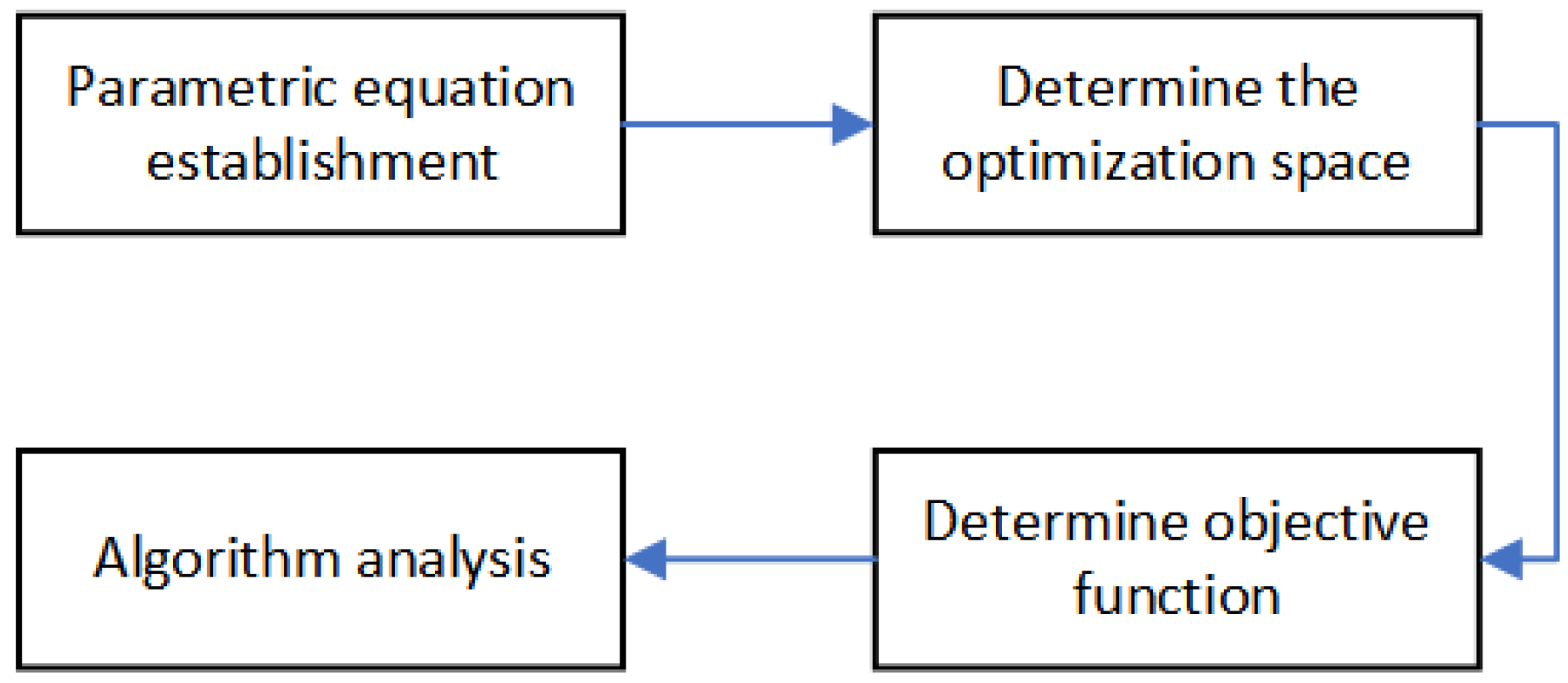
This section introduces the research process method, as shown in Figure 1. Firstly, parametric equations are established through the kinematic model; then, the optimization space of parameters and the objective function are determined, and, finally, the efficiency of the algorithm is analyzed.

2.1. Parameter Equation Path Considering Kinematic Model

The kinematics model of typical wheeled agricultural machinery can be described according to Equation (1):

$$\left\{\begin{array}{l}\dot{x}=v\cos \theta \\ \dot{y}=v\sin \theta \\ \dot{\theta }=\frac{v\tan \varphi }{l}\\ \dot{v}=acc\end{array}\right.$$

(1)

where $(x,y)$ represents the Cartesian coordinate of the middle point of the rear axle of agricultural machinery, $v$ represents the linear velocity of agricultural machinery, $\theta$ represents the heading angle of agricultural machinery, $\varphi$ represents the steering angle of agricultural machinery, $acc$ represents the acceleration of agricultural machinery, and $l$ is the wheel base.

For the given initial time and arrival time, agricultural machinery has initial constraints $q_0$ at $t_0$ and end constraints $q_f$ at $t_f$, where

$$\begin{array}{l}{q}_0=(x_0,y_0,{\theta }_0,{\varphi }_0,v_0,ac{c}_0)\\ q_f=(x_f,y_f,{\theta }_f,{\varphi }_f,v_f,ac{c}_f)\end{array}$$

(2)

In practical applications, the initial time $t_0$ is generally 0 and the other state constraints are the current state of the machinery. And, in the end constraint, since the radius of obstacles on the farm is generally much smaller than the desired path, the ideal path to avoid obstacles should be similar to the length of the desired path, so the end time $t_f$ can be calculated from the given initial and end positions and the average speed with Equation (3), which is defined in Equation (2):

$$t_f=\frac{2\sqrt{{(x_f-x_0)}^2+(y_f-y_0)}}{v_0+v_f}+t_a$$

(3)

where $t_a$ is an adjustable parameter that can be set to be larger for smooth operation and smaller for efficient operation of the machinery. In this way, the machinery is able to avoid obstacles by slightly accelerating. In addition, in order to ensure the stable state of the machine at the end, ${\varphi }_f$ and $ac{c}_f$ are set as 0.

Thus, the parameter equation path $x_d(t)$ should satisfy Equation (4) according to the initial and end limits:

$$\left\{\begin{array}{l}{x}_d(t_0)=x_0=h_1\\ {\dot{x}}_d(t_0)=v_0\cos {\theta }_0=h_2\\ {\ddot{x}}_d(t_0)=ac{c}_0\cos {\theta }_0-\frac{v_0^2\sin {\theta }_0\tan {\varphi }_0}{l}=h_3\\ x_d(t_f)=x_f=h_4\\ {\dot{x}}_d(t_f)=v_f\cos {\theta }_f=h_5\\ {\ddot{x}}_d(t_f)=ac{c}_f\cos {\theta }_f-\frac{v_f^2\sin {\theta }_f\tan {\varphi }_f}{l}=h_6\end{array}\right.$$

(4)

According to Equation (4), $x_d(t)$ needs 6 parameters at least. In the same way, $y_d(t)$ must satisfy a similar constraint. Adding one degree of freedom, the following polynomial trajectory is proposed:

$$\left\{\begin{array}{l}{x}_d(t)=a_0+a_{1}t+a_2{t}^2+a_3{t}^3+a_4{t}^4+a_5{t}^5+a_6{t}^6\\ y_d(t)=b_0+b_{1}t+b_2{t}^2+b_3{t}^3+b_4{t}^4+b_5{t}^5+b_6{t}^6\end{array}\right.$$

(5)

which defines:

$$\begin{array}{l}{x}_d(t_0)=h_1,y_d(t_0)=h_{11}\\ {\dot{x}}_d(t_0)=h_2,{\dot{y}}_d(t_0)=h_{12}\\ {\ddot{x}}_d(t_0)=h_3,{\ddot{y}}_d(t_0)=h_{13}\\ x_d(t_f)=h_4,y_d(t_f)=h_{14}\\ {\dot{x}}_d(t_f)=h_5,{\dot{y}}_d(t_f)=h_{15}\\ {\ddot{x}}_d(t_f)=h_6,{\ddot{y}}_d(t_f)=h_{16}\end{array}$$

(6)

Combining Equations (4) and (5):

$$\left\{\begin{array}{l}{a}_0+a_1{t}_0+a_2{t}_0^2+a_3{t}_0^3+a_4{t}_0^4+a_5{t}_0^5=h_1-a_6{t}_0^6\\ a_1+2a_2{t}_0+3a_3{t}_0^2+4a_4{t}_0^3+5a_5{t}_0^4=h_2-6a_6{t}_0^5\\ 2a_2+6a_3{t}_0+12a_4{t}_0^2+20a_5{t}_0^3=h_3-30a_6{t}_0^4\\ a_0+a_1{t}_f+a_2{t}_f^2+a_3{t}_f^3+a_4{t}_f^4+a_5{t}_f^5=h_1-a_6{t}_f^6\\ a_1+2a_2{t}_f+3a_3{t}_f^2+4a_4{t}_f^3+5a_5{t}_f^4=h_2-6a_6{t}_f^5\\ 2a_2+6a_3{t}_f+12a_4{t}_f^2+20a_5{t}_f^3=h_3-30a_6{t}_f^4\end{array}\right.$$

(7)

which can be described in matrix form:

$$L\overrightarrow{a}=H_1-M{a}_6$$

(8)

where

$$\begin{gathered} L=\left[\begin{array}{cccccc}1& t_0& t_0^2& t_0^3& t_0^4& t_0^5\\ 0& 1& 2t_0& 3t_0^2& 4t_0^3& 5t_0^4\\ 0& 0& 2& 6t_0& 12t_0^2& 20t_0^3\\ 1& t_f& t_f^2& t_f^3& t_f^4& t_f^5\\ 0& 1& 2t_f& 3t_f^2& 4t_f^3& 5t_f^4\\ 0& 0& 2& 6t_f& 12t_f^2& 20t_f^3\end{array}\right] \\ \overrightarrow{a}={[a_0,a_1,a_2,a_3,a_4,a_5]}^T \\ {H}_1={[h_1,h_2,h_3,h_4,h_5,h_6]}^T \\ M={[t_0^6,6t_0^5,30t_0^4,t_f^6,6t_f^5,30t_f^4]}^T \end{gathered}$$

$H_1$ is defined in Equation (6).

Similarly, $y_d(t)$ must satisfy:

$$L\overrightarrow{b}=H_2-M{b}_6,$$

(9)

where

$$\begin{gathered} \overrightarrow{b}={[b_0,b_1,b_2,b_3,b_4,b_5]}^T \\ {H}_2={[h_{11},h_{12},h_{13},h_{14},h_{15},h_{16}]}^T \end{gathered}$$

$H_2$ is defined in Equation (6).

For a practical mission, it is always true that $t_f>t_0$. Hence, the matrix L is nonsingular. Thus, $\overrightarrow{a}$ and $\overrightarrow{b}$ can be calculated via Equation (10):

$$\left\{\begin{array}{l}\overrightarrow{a}=L^{-1}(H_1-M{a}_6)\\ \overrightarrow{b}=L^{-1}(H_2-M{b}_6)\end{array}\right.$$

(10)

The planned trajectory $(x_d,y_d)$ can be rewritten as:

$$\left\{\begin{array}{l}{x}_d(t)=f(t)\overrightarrow{a}+a_6{t}^6=f(t)L^{-1}(H_1-M{a}_6)+a_6{t}^6\\ y_d(t)=f(t)\overrightarrow{b}+b_6{t}^6=f(t)L^{-1}(H_2-M{b}_6)+b_6{t}^6\end{array}\right.$$

(11)

where

$$f(t)=[1,t,t^2,t^3,t^4]$$

In short, given the initial constraints $q_0$ at $t_0$ and end constraints $q_f$ at $t_f$, fixed $a_6$ and $b_6$ give a path, satisfying the constraints mentioned above, which is described in Equation (11). The following algorithm optimizes $a_6$ and $b_6$ to obtain a path.

2.2. Definition of Search Space

Before using an optimization algorithm, defining an appropriate search space can help the algorithm find a relatively optimal solution faster. Therefore, it is necessary to first determine the search space of $a_6$ and $b_6$ to improve the solving efficiency of the optimization algorithm. To determine the search space, the search center and search radius for each variable need to be determined.

Determine the search center first. Generally, the objective function of a path planning algorithm is the path length:

$$J_s(x_d,y_d)={\displaystyle {\int }_{t_0}^{t_f}\sqrt{({\dot{x}}_d^2+{\dot{y}}_d^2)}dt}$$

(12)

However, since the objective function contains the square root, the optimal analytic solution cannot be derived directly. Therefore, the objective function is considered, as Equation (12) shows, which indicates that the path is expected to be a straight line from the starting point to the end point as far as possible.

$$J_l(x_d,y_d)={\displaystyle {\int }_{t_0}^{t_f}[{(x_d-x^{\prime })}^2+{(y_d-y^{\prime })}^2]dt}$$

(13)

where

$$\begin{gathered} \left\{\begin{array}{l}{x}^{\prime }=k_x(t-t_0)+x_0\\ y^{\prime }=k_y(t-t_0)+y_0\end{array}\right. \\ {k}_x=\frac{x_f-x_0}{t_f-t_0},k_y=\frac{y_f-y_0}{t_f-t_0} \end{gathered}$$

Expanding Equation (13):

$$\begin{array}{l}{J}_l={\displaystyle {\int }_{t_0}^{t_f}\{{[f(t)L^{-1}(H_1-M{a}_6)+a_6{t}^6-x^{\prime }]}^2+{[f(t)L^{-1}(H_2-M{b}_6)+b_6{t}^6-y^{\prime }]}^2\}dt}\\ ={\displaystyle {\int }_{t_0}^{t_f}[{(f_1{a}_6+f_2-x^{\prime })}^2+{(f_1{b}_6+f_3-y^{\prime })}^2]dt}\\ =p_1{a}_6^2+2p_2{a}_6+p_1{b}_6^2+2p_3{b}_6+p_4\\ =p_1{(a_6+\frac{p_2}{p_1})}^2+p_1{(b_6+\frac{p_3}{p_1})}^2+p_4-\frac{p_2^2}{p_1}-\frac{p_3^2}{p_1}\end{array}$$

(14)

where

$$\begin{gathered} f_1=t^6-f(t)L^{-1}M \\ {f}_2=f(t)L^{-1}{H}_1 \\ {f}_3=f(t)L^{-1}{H}_2 \\ {p}_1={\displaystyle {\int }_{t_0}^{t_f}{f}_1^{2}dt} \\ {p}_2={\displaystyle {\int }_{t_0}^{t_f}{f}_1(f_2-x^{\prime })dt} \\ {p}_3={\displaystyle {\int }_{t_0}^{t_f}{f}_1(f_3-y^{\prime })dt} \\ {p}_4={\displaystyle {\int }_{t_0}^{t_f}[{(f_2-x^{\prime })}^2+{(f_3-y^{\prime })}^2]dt} \end{gathered}$$

The optimal solution of Equation (13) is obtained:

$$\left\{\begin{array}{l}{a}_6^{*}=-\frac{p_2}{p_1}\\ b_6^{*}=-\frac{p_3}{p_1}\end{array}\right.$$

(15)

The optimal trajectory can be described as follows:

$$\left\{\begin{array}{l}{x}_d^{*}(t)=f(t)L^{-1}(H_1-M{a}_6^{*})+a_6^{*}{t}^6\\ y_d^{*}(t)=f(t)L^{-1}(H_2-M{b}_6^{*})+b_6^{*}{t}^6\end{array}\right.$$

(16)

An optimal analytical solution of the objective function can be obtained directly from Equation (16) efficiently. Therefore, $a_6^{*}$ and $b_6^{*}$ are chosen as the center of the search space of $a_6$ and $b_6$.

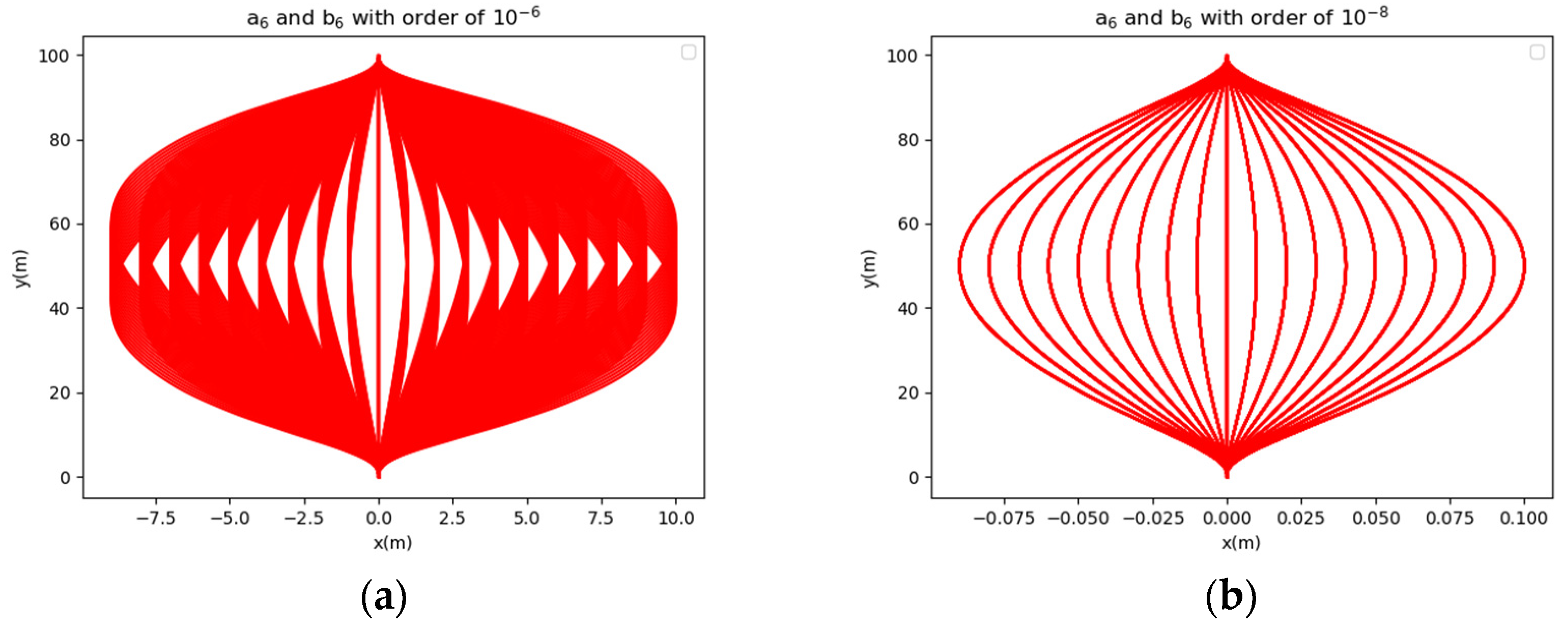
Then, the search radius is determined via quantitative experiments. Figure 2 shows the paths for different orders of $a_6$ and $b_6$. Figure 2a shows 100 paths when the values of $a_6$ and $b_6$ are set as an order of ${10}^{-6}$, which are within a range of 10 m. Figure 2b shows 100 paths when the values of $a_6$ and $b_6$ are set as an order of ${10}^{-8}$, which are within a range of 0.1 m. Quantitative experiments show that the order of $a_6$ and $b_6$ directly affects the scope of search paths, and the scope order of paths is linearly related to the order of $a_6$ and $b_6$. In addition, the value of $a_6$ and $b_6$ is also related to the total time; thus, different total times require a different search radius.

2.3. Particle Swarm Optimization

The particle swarm optimization algorithm [21] is a heuristic optimization algorithm that uses multiple particles to simulate the cooperation process of bird predation to find the solution that maximizes the value of the objective function. The focus of the particle swarm optimization algorithm is to determine the objective function and search space, which is described in Section 2.2. This section defines the objective function.

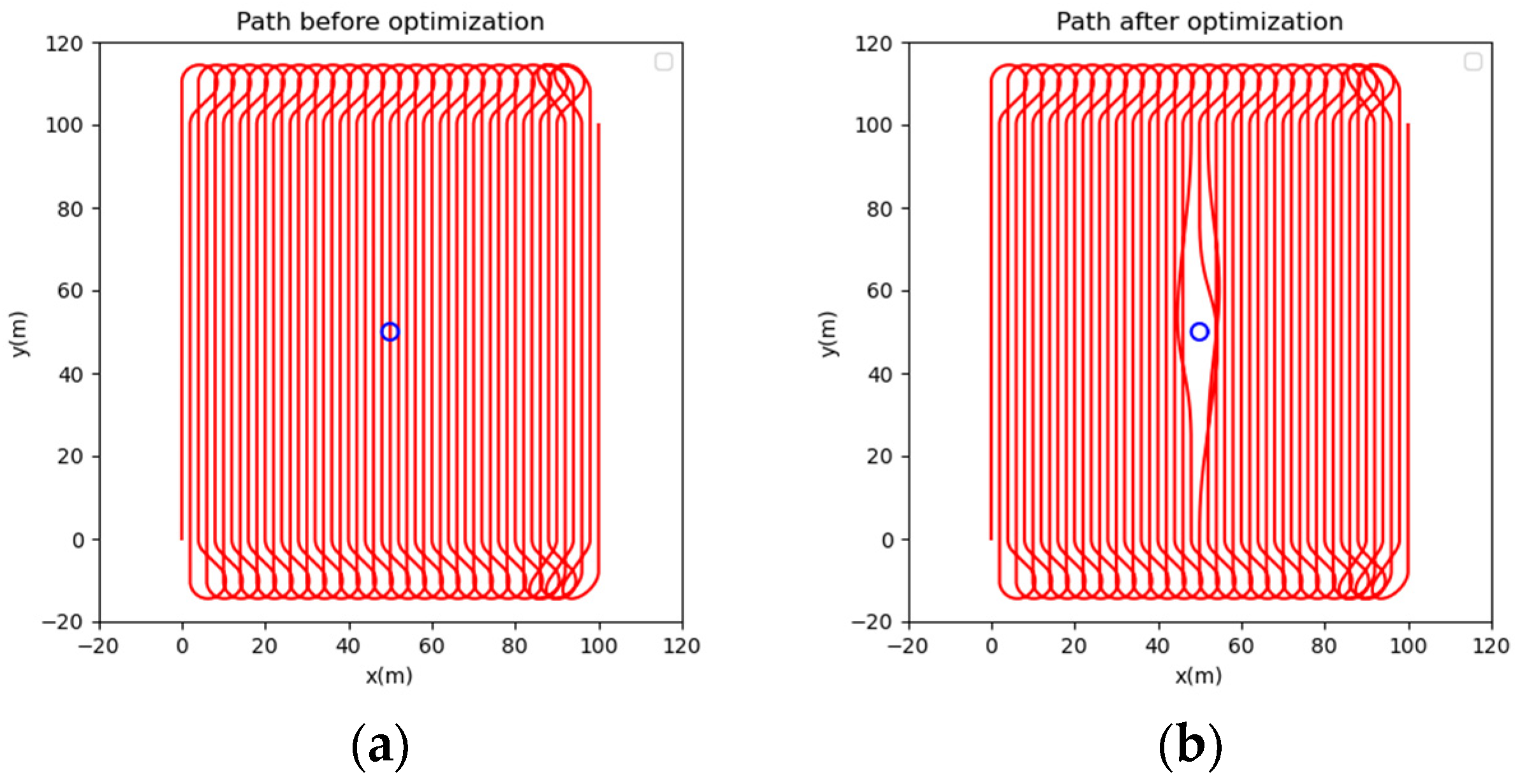
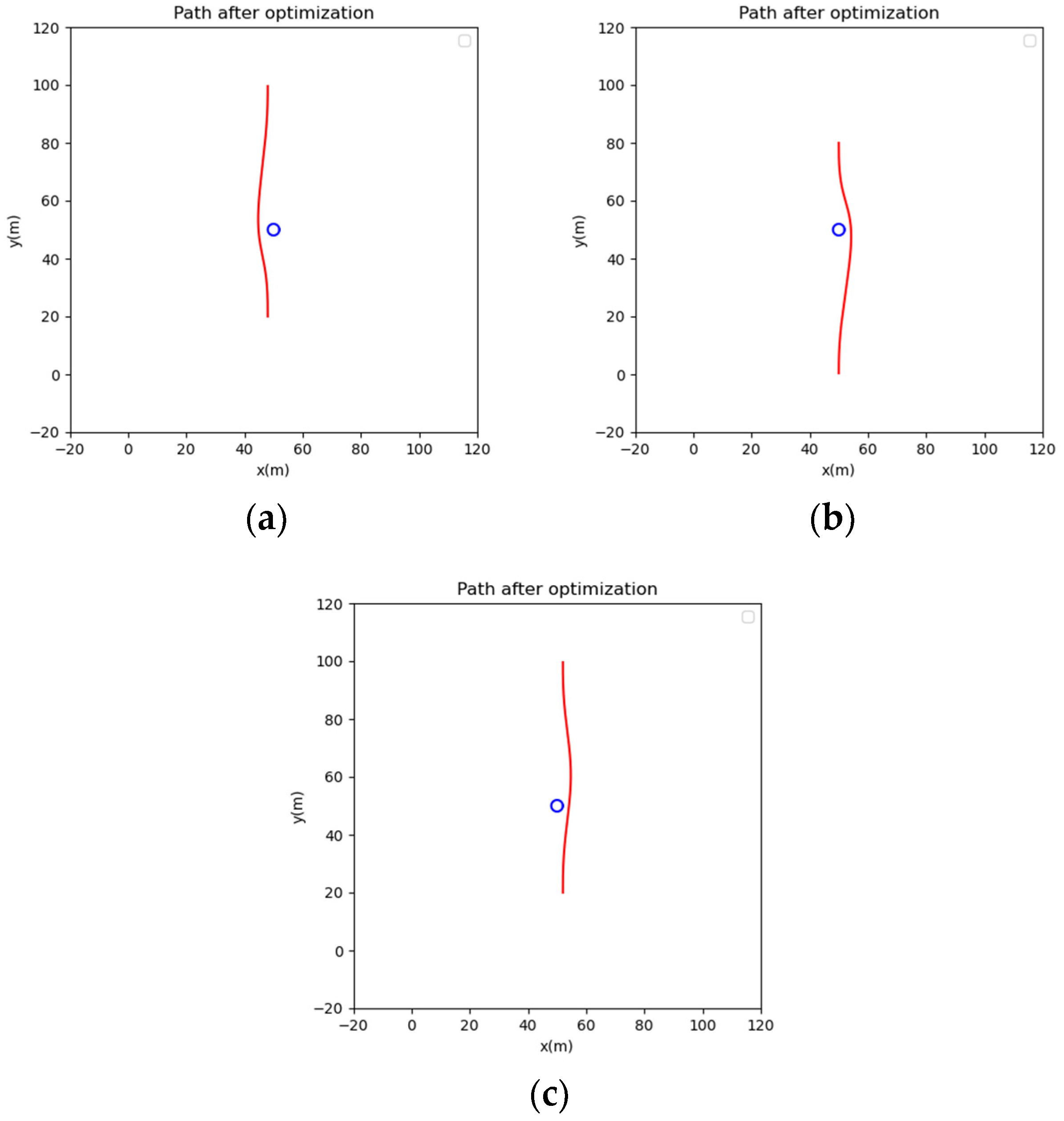
For a general path planning algorithm, the objective function is defined by Equation (12), and the objective of the optimization algorithm is to find the shortest path. However, due to the particularity of the work of unmanned agricultural machinery, the unmanned agricultural machinery is expected to avoid obstacles and, as far as possible, to keep itself running along the expected path to complete the task better. Therefore, two kinds of objective functions are defined, one defined by Equation (12) and the other defined by Equation (17), to find a path that minimizes the area enclosed by the path and the expected path.

$$J_a(x_d,y_d)={\displaystyle {\int }_{t_0}^{t_f}\frac{\left|A{x}_d-B{y}_d+C\right|\sqrt{{(B{\dot{x}}_d-A{\dot{y}}_d)}^2+C^2}}{\sqrt{A^2+B^2}}dt}$$

(17)

where $A,B,C$ are the parameters of the expected path $Ax+By+C=0$.

In addition, the path should satisfy the constraint of not colliding with obstacles. When the path of obstacles is known, the path needs to satisfy Equation (18).

$${[x_d(t)-x_{oi}(t)]}^2+{[y_d(t)-y_{oi}(t)]}^2\ge {(r_0+r_i)}^2,\forall t\in [t_0,t_f]$$

(18)

where $x_{oi}(t)$ and $y_{oi}(t)$ are the parametric equation of obstacles with respect to time, for $i=1,2,\dots ,n$, $r_0$ is the radius of the unmanned agricultural machinery, and $r_i$ is the radius of the obstacles, for $i=1,2,\dots ,n$. To meet the condition described above, define the objective function for avoiding obstacles, as in Equation (19).

$$J_{Ob}(x_d,y_d)=\left\{\begin{array}{l}0,\forall t\in [t_0,t_f],{[x_d(t)-x_{oi}(t)]}^2+{[y_d(t)-y_{oi}(t)]}^2\ge {(r_0+r_i)}^2\\ {10}^6,\exists t\in [t_0,t_f],{[x_d(t)-x_{oi}(t)]}^2+{[y_d(t)-y_{oi}(t)]}^2<{(r_0+r_i)}^2\end{array}\right.$$

(19)

where ${10}^6$ can be any number much larger than the length of the path, as the goal of path planning is to avoid obstacles first.

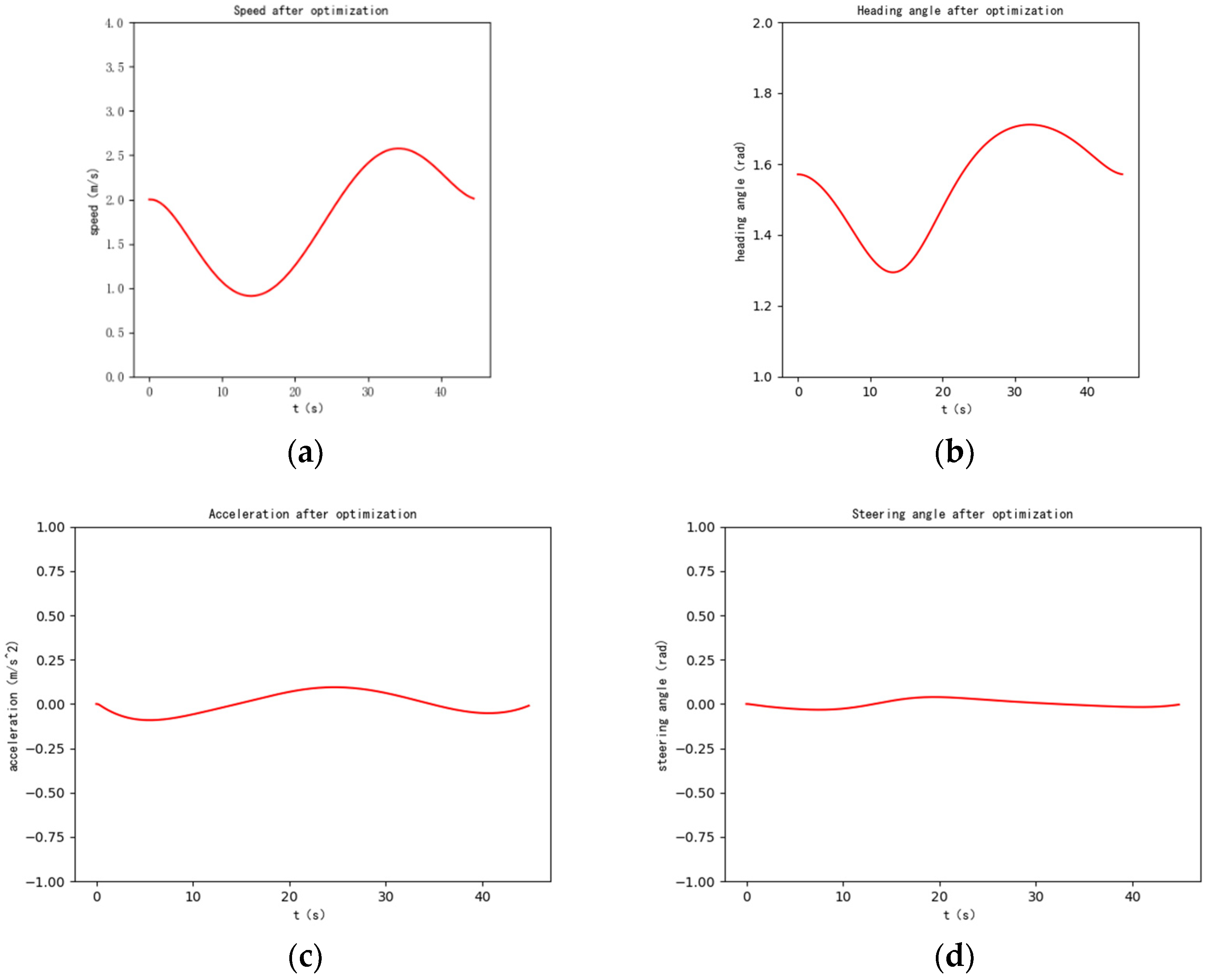
In addition, when determining the path, the acceleration and steering angle at each moment can be calculated according to the parametric equation of the path. According to the characteristics of the actual operation of agricultural machinery, acceleration constraints and steering angle constraints need to be added, which are expressed by Equation (20) and Equation (21), respectively.

$$J_{acc}=\left\{\begin{array}{l}0,\forall t\in [t_0,t_f],ac{c}_{ll}\le acc(t)\le ac{c}_{ul}\\ {10}^6,\exists t\in [t_0,t_f],acc(t)<ac{c}_{ll}|acc(t)>ac{c}_{ul}\end{array}\right.$$

(20)

$$J_{\varphi }=\left\{\begin{array}{l}0,\forall t\in [t_0,t_f],{\varphi }_{ll}\le \varphi (t)\le {\varphi }_{ul}\\ {10}^6,\exists t\in [t_0,t_f],\varphi (t)<{\varphi }_{ll}|\varphi (t)>{\varphi }_{ul}\end{array}\right.$$

(21)

where $ac{c}_{ll}$ and $ac{c}_{ul}$ represent the lower limit and the upper limit of acceleration for agricultural machinery; ${\varphi }_{ll}$ and ${\varphi }_{ul}$ represent the lower limit and the upper limit of the steering angle for agricultural machinery.

Based on the above constraints and objective functions, the objective function of the particle swarm optimization algorithm is represented by Equation (22) when the path length is selected as the target and by Equation (23) when the target is to find a path close to the expected path.

$$J_{PSO1}(x_d,y_d)=-J_s-J_{\mathit{acc}}-J_{\varphi }$$

(22)

$$J_{PSO2}(x_d,y_d)=-J_a-J_{\mathit{acc}}-J_{\varphi }$$

(23)

It is worth noting that when the optimization result of the objective function value is greater than the preset large number, it means that the current optimization algorithm has not found a path to avoid obstacles, while when the optimization result of the objective function value is less than the preset large number, it means that the current optimization algorithm has found a path to avoid obstacles and is relatively better. For the optimization algorithm, avoiding obstacles is the priority, so it has a large penalty. Only when the path does not conflict with the obstacle, other objective functions of the optimized path are considered. In addition, since the parametric equation of obstacle with time is used in $J_{Ob}(x_d,y_d)$, this optimization method can theoretically avoid any dynamic obstacle with a known trajectory, but for an obstacle with too large a radius, it needs to search in a larger search space with a higher end time, so that the algorithm can plan the path that the agricultural machine can achieve. Considering the actual farm scene, it is considered that the radius of the obstacle is far less than the path length, so it is feasible in practical application. What is more, the end speed and end heading angle can also be used as search variables, which can help the optimization algorithm find the second-best solution when the obstacle is close to the end point and still reach the end point with a small deviation in the speed and heading angle, and then the control algorithm can be used to complete the desired path tracking.

2.4. Algorithm Efficiency Analysis

In the running process of the algorithm, the initial solution is solved first. Since the analytical solution is directly solved, the running time is short, about 0.002 s. The main time cost of the algorithm is the process of solving the objective function in the following particle swarm optimization algorithm. As described in Section 2.3, the objective function needs discrete calculation, so the calculation of the objective function is related to the total time and discrete time. In addition, obstacle collision detection is also related to the number of obstacles. The number of iterations and populations in the particle swarm optimization algorithm determines the calculation times of the objective function. In short, the running time of the algorithm is positively correlated with the total time, the number of iterations, and the number of populations, and it is negatively correlated with the discrete time. The number of obstacles has little influence on the running time of the algorithm compared with other factors.

2.5. Influence of Discrete Time on Obstacle Collision Detection

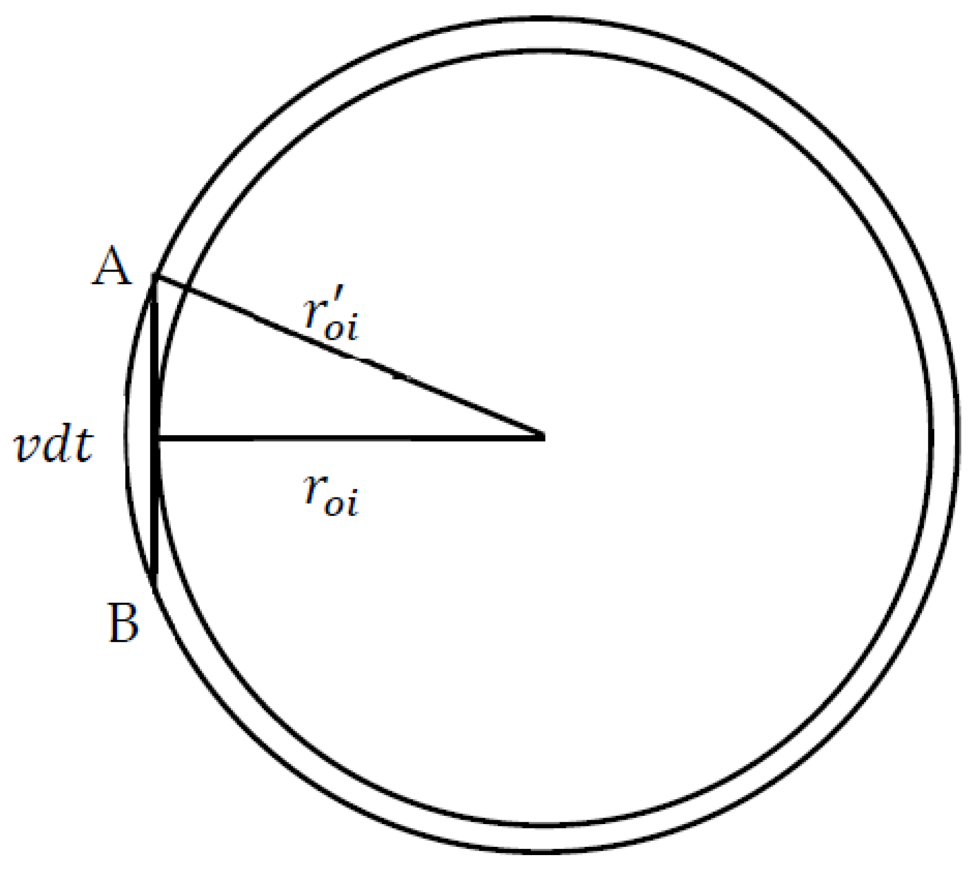
In obstacle collision detection, agricultural machinery coordinates and obstacle coordinates cannot be detected at every moment, so it is necessary to conduct obstacle detection after the discretization of the agricultural machinery path and obstacle path. Therefore, the discrete time has an impact on obstacle detection. In the past, the radius of the obstacle or the collision radius of the moving subject was generally expanded. In this section, the expanded value was quantitatively defined.

As shown in Figure 3, the worst case of collision detection after discretization is that discretized points A and B are close to obstacles, and then the compensation value $r_{oi}^{\prime }$ can be calculated via Equation (24).

$$r_{oi}^{\prime }=\sqrt{r_{oi}^2+{(\frac{vdt}{2})}^2}$$

(24)

where $v$ is the mean speed, and $dt$ is the discrete time. In addition, $vdt$ cannot be greater than the minimum diameter of all obstacles; otherwise, collision detection may fail.

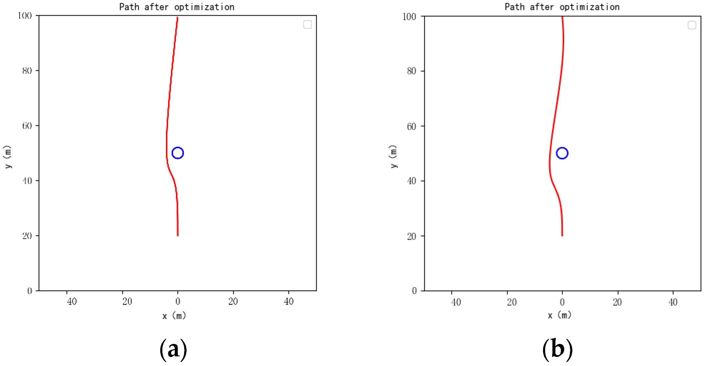
3. Experiments

This section presents the simulation results of the proposed algorithm. The algorithm was run on a personal computer with AMD Ryzen 5 4600H with Radeon [email protected] GHz CPU, 16 GB of RAM, 64-bit Windows 10 professional operating system, and running in python. It should be noted that python is inefficient, and the speed of the algorithm can be further improved if executed in C++, although the algorithm in python is already running at the required speed. In addition, since the average speed of unmanned agricultural machines is only 2 m/s, the discretization step size is selected as 0.5 s, which can be changed. However, too short a discretization step size would lead to inefficiency, and too long a discretization step size will lead to inaccurate objective function value and collision judgement. The wheelbase of unmanned agricultural machinery is set as 3 m. The collision radius of agricultural machinery is set as 2 m, and the distance of obstacle detection of agricultural machinery is set as 30 m. Due to the particularity of unmanned agricultural machinery operation, the following experiments utilizes Equation (23) as objective function.

3.1. Static Obstacle Avoidance Experiment

Before the operation of unmanned agricultural machinery, the global path is planned by the complete path planning algorithm. As shown in Figure 4a, the operating area of the unmanned agricultural machinery is a rectangle farm 100 m long and 100 m wide, and the global path is represented by the red curve. The unmanned agricultural machinery runs straight along the crop line in the operating area. When it reaches the edge of the operating area, it turns around and enters the next crop line. Suppose that the farm contains a static obstacle with a radius of 2 m in (50, 50).

Figure 4b shows the actual driving path of the unmanned agricultural machinery after its full operation. Before detecting an obstacle or detecting an obstacle that will not collide, the unmanned agricultural machinery runs according to the global path. When the agricultural machinery reaches (48, 20), it is 30 m away from the obstacle and detects the obstacle that will collide with the agricultural machinery if it continues to run. Therefore, the algorithm runs for the first time with initial constraints and end constraints set as follows:

$$t_0=0,q_0=[48,20,\frac{\pi }{2},0,2,0],t_f=45,q_f=[48,100,\frac{\pi }{2},0,2,0]$$

The population of the particle swarm optimization algorithm is set as 10, the number of iterations is set to 10, and the running time is 0.5 s. The result path is shown in Figure 5a. Agricultural machinery runs along this path and continues to run along the global path after arriving at (48, 100). When the agricultural machinery reaches (50, 80), it is 30 m away from the obstacle and detects the obstacle that will collide with the agricultural machinery if it continues to run. Therefore, the algorithm runs for the second time with initial constraints and end constraints set as follows:

$$t_0=0,q_0=[50,80,-\frac{\pi }{2},0,2,0],t_f=45,q_f=[50,0,-\frac{\pi }{2},0,2,0]$$

The other parameters are set to be the same as the first time, and the running time is the same. The result path is shown in Figure 5b. Agricultural machinery runs along this path and continues to run along the global path after arriving at (50, 0). When the agricultural machinery reaches (52, 20), it is 30 m away from the obstacle and detects the obstacle that will collide with the agricultural machinery if it continues to run. Therefore, the algorithm runs for the third time with initial constraints and end constraints set as follows:

$$t_0=0,q_0=[52,20,\frac{\pi }{2},0,2,0],t_f=45,q_f=[52,100,\frac{\pi }{2},0,2,0]$$

The other parameters are set the same as the first time, and the running time is the same. The result path is shown in Figure 5c. Agricultural machinery runs along this path and continues to run along the global path after arriving at (52, 100).

In order to prove that the path planned by the proposed algorithm conforms to the dynamic model, the velocity, heading angle, acceleration, and steering angle of the path at x equal to 50 are shown in Figure 6. All of them have good conductibility and are within the expected range, in accordance with the kinematic model of unmanned agricultural machinery.

3.2. Dynamic Obstacle Avoidance Experiment

In practical application, dynamic obstacles are detected and tracked via computer vision. After obtaining continuous spatial coordinates of a certain time, the motion trajectory of dynamic obstacles is estimated, and a parametric equation with time as a parameter is generated, as shown in the following equation. After estimating the motion trajectory, collision detection is performed first. If a collision occurs, the algorithm is run to obtain the obstacle avoidance path trajectory; otherwise, the algorithm is not run. It should be emphasized that the parameter $t$ of the above parametric equation is unified with the initial time $t_0$ in the algorithm; that is, the coordinate obtained in the parametric equation when $t$ is equal to $t_0$ is the same as the coordinate of the dynamic obstacle at the initial time. When the algorithm is used, $t_0$ is usually set as 0; then, the constant term of the parametric equation is the dynamic obstacle coordinate when the algorithm is run, and the coefficient of the primary term is the dynamic obstacle velocity component estimated by the continuous coordinate of the dynamic obstacle in a period of time before the algorithm is used.

$$\left\{\begin{array}{l}{x}_{oi}=x_{oi0}+v_{oix}(t-t_0)\\ y_{oi}=y_{oi0}+v_{oiy}(t-t_0)\end{array}\right.$$

Suppose that there is a dynamic obstacle with a radius of 2 m, whose equation of locus is as follows:

$$\left\{\begin{array}{l}{x}_{o1}=-50+3.6t\\ y_{o1}=50\end{array}\right.$$

The initial constraints and end constraints are set as:

$$t_0=0,q_0=[50,20,\frac{\pi }{2},0,2,0],t_f=45,q_f=[50,100,\frac{\pi }{2},0,2,0]$$

The path before optimization and path, speed, and heading angle after optimization is shown in Figure 7. When facing a dynamic obstacle, due to the setting of the objective function, the algorithm preferentially avoids obstacles by adjusting the running speed of agricultural machinery, in which case, the objective function value remains optimal, while the objective function values will be sub-optimal if the path is altered. As shown in Figure 7a, before optimization, the agricultural machinery is closest to the dynamic obstacle at 18 s and collision occurs. In Figure 7b, the position of the agricultural machinery and the dynamic obstacle is shown at 18 s, and no collision occurs. As shown in Figure 7c, the agricultural machinery first slows down to wait for the obstacle to leave the expected path and then accelerates to the normal speed to reach the target point. As shown in Figure 7d, the heading angle is almost unchanged. It is worth mentioning that if the radius of the dynamic obstacle is too large and the agricultural machinery decelerates to zero but still cannot avoid the collision with the obstacle, the algorithm will plan a path for the agricultural machinery to avoid the dynamic obstacle by changing the moving path of the agricultural machinery.

3.3. Comparison for Algorithm with Two Objective Functions

An experiment for comparing the algorithm with two objective functions is carried out. When facing a static obstacle with a radius of 2 m in (50, 50), the results of the algorithm with two objective functions are shown in Figure 8.

As shown in Figure 8a, agricultural machinery remains straight to the goal point, while in Figure 8b, agricultural machinery drives back to the desired path, which meets the requirements of agricultural machinery. So, the objective function defined by Equation (17) is normally used in agricultural machinery, while the objective function defined by Equation (12) can be used in other fields.

3.4. Comparison with Other Algorithms

An experiment comparing the proposed algorithm with classical path planning algorithms is carried out. Facing the same static obstacle with a radius of 2 m in (50, 50), the results of the A* algorithm and an analytical algorithm [16] for parametric path are shown below.

As shown in Figure 9a, the path planned by A* algorithm is not differentiable, which means not feasible for agricultural machinery. What’s more, the path also cannot meet the requirements of agricultural machinery operation. As shown in Figure 9b, the path planned using the analytical method in [16] for the parametric path is feasible, and the algorithm is extremely efficient. But it cannot meet the requirements of agricultural machinery as well. Comparing with two typical algorithms, the proposed algorithm combines the advantages of both. The path is feasible and satisfies the kinematic model. The design of the objective function also makes the algorithm flexible for different scenes.

3.5. Experiments for PSO Parameters

Epochs and the number of populations are the most important parameters in PSO. In order to further study the effect of the parameters of PSO on the results of the proposed algorithm, experiments are carried out. In experiments, other parameters are the same as above.

As is shown in

Table 1. Experiments of different PSO parameters.

Parameters Set	Time Consumed (s)	Value of Objective Function
Epochs = 1, Num = 1	0.01	Fail
Epochs = 1, Num = 5	0.04	153
Epochs = 1, Num = 10	0.08	137
Epochs = 1, Num = 20	0.15	120
Epochs = 5, Num = 1	0.04	Fail
Epochs = 5, Num = 5	0.14	139
Epochs = 5, Num = 10	0.28	138
Epochs = 5, Num = 20	0.55	119
Epochs = 10, Num = 1	0.08	Fail
Epochs = 10, Num = 5	0.28	136
Epochs = 10, Num = 10	0.53	130
Epochs = 10, Num = 20	1.02	116
Epochs = 20, Num = 1	0.15	Fail
Epochs = 20, Num = 5	0.54	134
Epochs = 20, Num = 10	1.03	127
Epochs = 20, Num = 20	2.01	112

, with the increase in the epochs and the number of populations in the algorithm, the time consumed is increasing, and the algorithm can find better solutions. It can be seen that when the number of populations is too small, the population path may be randomly initialized to solutions that do not satisfy the constraints, leading to optimization failure. Increasing the number of populations has a more profound effect on the results of the algorithm than epochs.

4. Conclusions

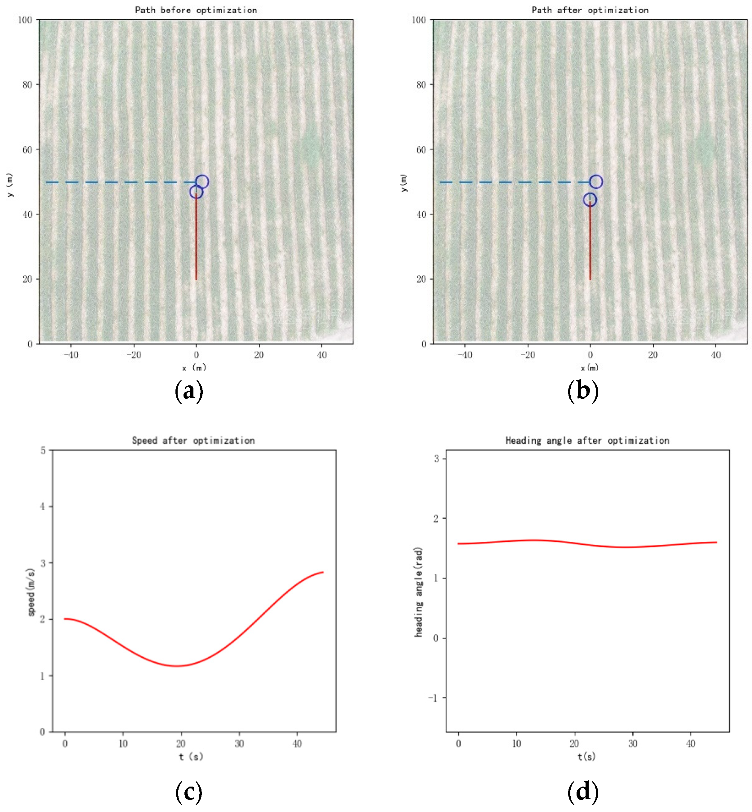
In this paper, the kinematic model of agricultural machinery is used to construct a parametric curve under the initial constraints and end constraints. The curve contains two degrees of freedom, $a_6$ and $b_6$. On this basis, firstly, the center of the search space is obtained directly via the analytical method. Through quantitative experiments, the search radius is determined. Then, the particle swarm optimization algorithm is used to optimize the path that satisfies the constraints of obstacles, acceleration, and steering angle and has relatively optimal objective function value. The objective function can select the length of the path, the area enclosed by the path, and the expected path. And the algorithm’s operating efficiency and the effect of discrete time on obstacle collision detection are analyzed. Finally, the effectiveness and real-time performance of the algorithm for static and dynamic obstacles are verified through experiments.

The uniqueness of the proposed algorithm is that it is aimed at the working purpose of the actual operation of agricultural machinery, while other obstacle avoidance path planning algorithms limit the optimization objective to the path length or operation efficiency. In addition, the proposed algorithm can satisfy the kinematic model constraints, and the planned path is feasible, directly controlled by algorithms. Although the proposed algorithm can obtain better obstacle avoidance path planning results in simulation, the parameterized path method still has limitations. Some parameters such as termination time need to be set manually. Therefore, more effective automatic setting methods of such parameters can be explored in the future.

References

1. Masehian, E.; Amin-Naseri, M.R. A voronoi diagram-visibility graph-potential field compound algorithm for robot path planning. J. Robot. Syst. 2004, 21, 275–300. [Google Scholar]
2. Wang, X.; Quan, L.I.; Guo, Q.; He, W.U.; Fu, F.U. The generalization and construction of Voronoi diagram and its application on delimitating city’s affected coverage. J. Cent. China Norm. Univ. 2002, 36, 107–111. [Google Scholar]
3. Dijkstra, E.W. Two problems in connection with graphs. Numer. Math. 1959, 1, 269–271. [Google Scholar] [CrossRef]
4. Hart, P.E.; Nilsson, N.J.; Raphael, B. A formal basis for the heuristic determination of minimum cost paths. IEEE Trans. Syst. Sci. Cybern. 1968, 4, 100–107. [Google Scholar] [CrossRef]
5. Stentz, A. Optimal and efficient path planning for partially-known environments. In Proceedings of the IEEE International Conference On Robotics and Automation, San Diego, CA, USA, 8–13 May 1994; Volume 1, p. 3310. [Google Scholar]
6. Stentz, A. The focused D* Algorithm for Real-Time Replanning. In Proceedings of the International Joint Conference on Artificial Intelligence, Vienna, Austria, 23–29 July 2000. [Google Scholar]
7. Li, X.; Hu, X.; Wang, Z.; Du, Z. Path Planning Based on Combination of Improved A-STAR Algorithm and DWA Algorithm. In Proceedings of the 2nd International Conference on Artificial Intelligence and Advanced Manufacture (AIAM), Manchester, UK, 15–17 October 2020. [Google Scholar]
8. Zhang, Z.; Wu, J.; Dai, J.; He, C. Optimal path planning with modified A-Star algorithm for stealth unmanned aerial vehicles in 3D network radar environment. J. Aerosp. Eng. 2022, 236, 72–81. [Google Scholar]
9. Kim, J.; Ostrowski, J.P. Motion planning of aerial robot using rapidly-exploring random trees with dynamic constraints. In Proceedings of the 20th IEEE International Conference on Robotics and Automation (ICRA), Taipei, Taiwan, 14–19 September 2003. [Google Scholar]
10. Wang, H.; Li, G.; Hou, J.; Chen, L.; Hu, N. A Path Planning Method for Underground Intelligent Vehicles Based on and Improved RRT* Algorithm. Electronics 2022, 11, 294. [Google Scholar] [CrossRef]
11. Khatib, O. Real-time obstacle avoidance for manipulators and mobile robots. Int. J. Robot. Res. 1990, 5, 90–98. [Google Scholar] [CrossRef]
12. Borenstein, J.; Koren, Y. The vector field histogram-fast obstacle avoidance for mobile robots. IEEE Trans. Robot. Autom. 1991, 7, 278–288. [Google Scholar] [CrossRef]
13. Yuan, H.; Qu, Z. Optimal real-time collision-free motion planning for autonomous underwater vehicles in a 3D underwater space. IET Control Theory Appl. 2009, 3, 712–721. [Google Scholar] [CrossRef]
14. Qu, Z.; Jing, W.; Plaisted, C.E. A new analytical solution to mobile robot trajectory generation in the presence of moving obstacles. IEEE Trans. Robot. 2004, 20, 978–993. [Google Scholar] [CrossRef]
15. Yang, J.; Daoui, A.; Qu, Z.; Wang, J.; Hull, R.A. An Optimal and Real-Time Solution to Parameterized Mobile Robot Trajectories in the Presence of Moving Obstacles. In Proceedings of the 2005 IEEE International Conference on Robotics and Automation, Barcelona, Spain, 18–22 April 2005. [Google Scholar]
16. Yuan, H.; Shim, T. Model based real-time collision-free motion planning for mobile robots in unknown dynamic environments. In Proceedings of the 2011 14th International IEEE Conference on Intelligent Transportation Systems (ITSC), Washington, DC, USA, 5–7 October 2011. [Google Scholar]
17. Kuo, Y.L.; Lin, C.C.; Lin, Z.T. Dual-optimization trajectory planning based on parametric curves for a robot manipulator. Int. J. Adv. Robot. Syst. 2020, 17, 1135–1145. [Google Scholar] [CrossRef]
18. Ghosh, D.; Nandakumar, G.; Narayanan, K.; Honkote, V.; Sharma, S. Kinematic Constraints Based Bi-directional RRT (KB-RRT) with Parameterized Trajectories for Robot Path Planning in Cluttered Environment. In Proceedings of the 2019 International Conference on Robotics and Automation (ICRA), Montreal, QC, Canada, 20–24 May 2019. [Google Scholar]
19. Essaidi, A.B.; Haddad, M.; Lehtihet, H.E. Minimum-time trajectory planning under dynamic constraints for a wheeled mobile robot with a trailer. Mech. Mach. Theory 2022, 169, 104605. [Google Scholar]
20. Faroni, M.; Beschi, M.; Guarino, C.; Visioli, A. Predictive joint trajectory scaling for manipulators with kinodynamic constraints. Control Eng. Pract. 2019, 95, 104264. [Google Scholar]
21. Chen, G.C.; Jin-Shou, Y.U. Particle Swarm Optimization Algorithm. Inf. Control 2005, 186, 454–458. [Google Scholar]
22. Kun, H. Path Planning of Mobile Robot Based on Improved Obstacle Avoidance Strategy and Double Optimization Ant Colony Algorithm. Trans. Chin. Soc. Agric. Mach. 2022, 53, 8. [Google Scholar]
23. Xue, H. A quasi-reflection based SC-PSO for ship path planning with grounding avoidance. Ocean. Eng. 2022, 247, 110772. [Google Scholar] [CrossRef]
24. Xu, L.; Cao, M.; Song, B. A new approach to smooth path planning of mobile robot based on quartic Bezier transition curve and improved PSO algorithm. Neurocomputing 2022, 473, 98–106. [Google Scholar] [CrossRef]
25. Chen, M.; Sharma, A.; Bhola, J.; Nguyen, T.V.T.; Truong, C.V. Multi-agent task planning and resource apportionment in a smart grid. Int. J. Syst. Assur. Eng. Manag. 2022, 13, 444–455. [Google Scholar] [CrossRef]
26. Kler, R.; Gangurde, R.; Elmirzaev, S.; Hossain, M.S.; Vo, N.V.; Nguyen, T.V.; Kumar, P.N. Optimization of Meat and Poultry Farm Inventory Stock Using Data Analytics for Green Supply Chain Network. Discret. Dyn. Nat. Soc. 2022, 2022, 8970549. [Google Scholar] [CrossRef]
27. Wang, C.N.; Yang, F.C.; Vo, T.M.N.; Nguyen, V.T.T.; Singh, M. Enhancing Efficiency and Cost-Effectiveness: A Groundbreaking Bi-Algorithm MCDM Approach. Appl. Sci. 2023, 13, 9105. [Google Scholar]
28. Liu, C.; Zhao, X.; Du, Y.; Cao, C.; Zhu, Z.; Mao, E. Research on static path planning method of small obstacles for automatic navigation of agricultural machinery. IFAC-PapersOnLine 2018, 51, 673–677. [Google Scholar] [CrossRef]
29. Zhao, X.; Wang, K.; Wu, S.; Wen, L.; Chen, Z.; Dong, L.; Sun, M.; Wu, C. An obstacle avoidance path planner for an autonomous tractor using the minimum snap algorithm. Comput. Electron. Agric. 2023, 207, 107738. [Google Scholar] [CrossRef]
Figure 1. Study flow chart.
Agriculture 13 01960 g001
Figure 2. Path with different a 6 and b 6 . (a) a 6 and b 6 with order of 10 6 . (b) a 6 and b 6 with order of 10 8 .
Agriculture 13 01960 g002
Figure 3. Influence of discrete time on obstacle collision detection.
Agriculture 13 01960 g003
Figure 4. Path before and after optimization for static obstacle. (a) Path before optimization. (b) Path after optimization.
Agriculture 13 01960 g004
Figure 5. Three paths after optimization for static obstacle. (a) Path at x is equal to 48. (b) Path at x is equal to 50. (c) Path at x is equal to 52.
Agriculture 13 01960 g005
Figure 6. State variables of path after optimization. (a) Speed curve. (b) Heading angle curve. (c) Acceleration curve. (d) Steering angle curve.
Agriculture 13 01960 g006
Figure 7. Path before and after optimization and its speed and heading angle. (a) Path before optimization. (b) Path after optimization. (c) Speed after optimization. (d) Heading angle after optimization.
Agriculture 13 01960 g007
Figure 8. Comparison for algorithm with two objective functions. (a) Path after optimization with objective function defined by Equation (12). (b) Path after optimization with objective function defined by Equation (17).
Agriculture 13 01960 g008
Figure 9. Comparison with other algorithms. (a) Path planned by A* algorithm. (b) Path planned by analytical method for parametric path.
Agriculture 13 01960 g009