Article

Applying RGB-Based Vegetation Indices Obtained from UAS Imagery for Monitoring the Rice Crop at the Field Scale: A Case Study in Portugal

by
Romeu Gerardo
1,2,3 and
Isabel P. de Lima
1,4,*
1
Department of Civil Engineering, Faculty of Sciences and Technology, University of Coimbra, Rua Luís Reis Santos, 3030-788 Coimbra, Portugal
2
CERIS–Civil Engineering Research and Innovation for Sustainability, University of Coimbra, Rua Pedro Hispano s/n, 3030-289 Coimbra, Portugal
3
Itecons, Rua Pedro Hispano, 3030-289 Coimbra, Portugal
4
MARE—Marine and Environmental Sciences Centre/ARNET—Aquatic Research Network, University of Coimbra, Rua Sílvio Lima, 3030-790 Coimbra, Portugal
*
Author to whom correspondence should be addressed.
Agriculture 2023, 13(10), 1916; https://doi.org/10.3390/agriculture13101916
Submission received: 5 September 2023 / Revised: 20 September 2023 / Accepted: 25 September 2023 / Published: 29 September 2023

Abstract

:
Nowadays, Unmanned Aerial Systems (UASs) provide an efficient and relatively affordable remote sensing technology for assessing vegetation attributes and status across agricultural areas through wide-area imagery collected with cameras installed on board. This reduces the cost and time of crop monitoring at the field scale in comparison to conventional field surveys. In general, by using remote sensing-based approaches, information on crop conditions is obtained through the calculation and mapping of multispectral vegetation indices. However, some farmers are unable to afford the cost of multispectral images, while the use of RGB images could be a viable approach for monitoring the rice crop quickly and cost-effectively. Nevertheless, the suitability of RGB indices for this specific purpose is not yet well established and needs further investigation. The aim of this work is to explore the use of UAS-based RGB vegetation indices to monitor the rice crop. The study was conducted in a paddy area located in the Lis Valley (Central Portugal). The results revealed that the RGB indices, Visible Atmospherically Resistant Index (VARI) and Triangular Greenness Index (TGI) can be useful tools for rice crop monitoring in the absence of multispectral images, particularly in the late vegetative phase.

1. Introduction

Rice (Oryza sativa L.) is one of the most important grain crops worldwide; it serves as a food staple for more than half of the world’s population [1,2] and is one of the most important sources of the rural population’s livelihood and income. However, a lack of technical efficiency often has a negative impact on rice productivity, which can affect agricultural incomes [3]. One main difficulty is the deficient monitoring tools and data available that have been limiting the full understanding of the relationships between hydrological conditions and agronomic management decisions and crop yields, which is key to optimizing profits and the sustainability of the agricultural sector. Currently, remote sensing (RS) is being widely used for crop growth monitoring. RS methodologies show important advantages: they are non-destructive, time- and cost-efficient, and they allow us to monitor vegetation conditions over broader spatial extents. Recent RS technological improvements have been appraised in many studies that report the high efficiency and accuracy of RS products for this end [4,5,6,7]. RS techniques rely mainly on the relationship between plants’ (and canopies’) optical properties and bio-physiological parameters [8,9], with a focus on water and nutrients’ use efficiency [10,11].
RS typically uses multispectral (MS) sensors to conduct observations of terrestrial surfaces and targeted objects [12,13]; these sensors are usually mounted on aerial systems (e.g., Unmanned Aerial Systems, UASs) and satellites (e.g., Sentinel-2). Satellite RS provides cost-effective MS and multi-temporal data, as well as wide spatial coverage. However, although the spatial resolution of open satellite images and data has been increasing (e.g., Sentinel-2), their resolution does not yet sufficiently satisfy the needs of precision agriculture. Precision agriculture aims to establish crop inputs in agronomic management according to within-field requirements to increase profitability while protecting the environment, and RS proves particularly valuable in pinpointing areas that require additional treatment with water, chemicals, pesticides, and herbicides. Moreover, satellite data availability could be affected by infrequent revisit times and cloud cover. On the other hand, recent advances in micro-technologies have significantly advanced the use of UASs for acquiring environmental data remotely [14]. UASs typically fly at low altitudes, offering the possibility to complement systems that operate at high altitudes while providing complementary sources of higher resolution information [15]. UAS sensors offer unique opportunities to bridge the existing gap between proximal field observations and air- and space-borne RS by providing high-spatial detail over relatively large areas cost-effectively, while allowing enhanced temporal data retrieval [14,16]. UAS-based imagery contributes valuably to increasing our knowledge about surface processes and land cover dynamics and is presently providing innovative approaches and solutions for crop management and monitoring in agricultural fields, among other applications [14,17]. Through available high-resolution MS images from UASs, managers and specialists in agriculture gain access to better quality information on field and crop conditions, which is key to improving management decisions and formulating precision farming solutions [18]. In fact, one of the most economically important sectors for the application of UASs is precision agriculture [19].
Nonetheless, the widespread integration of remote sensing into precision agriculture depends on factors such as affordability, accessibility, and the resolution of the imagery. MS sensors are relatively more expensive and inaccessible in low-income countries, where the agricultural sector is dominant, than in countries with more favorable economic and technological conditions. This limitation hinders the use of UASs-based RS tools by farmers in those countries. On the other hand, the widespread availability of UASs equipped with common real-image cameras (i.e., RGB cameras, which use the Red, Green and Blue channels), and the fact that high-resolution RGB cameras are presently more reasonably priced than in the past, make them overall more affordable than MS cameras. This has recently started to be seen as an opportunity for vegetation and crop monitoring [19,20,21]. The price range for MS cameras and RGB cameras suitable for precision agriculture can vary widely based on factors like brand, specifications, and additional features. MS cameras can cost, on average, $2000 for entry-level models and $15,000 or more for high-end cameras. Entry-level RGB cameras can vary in price, with an average cost of around $1000, while high-end RGB cameras can be priced at $7000 or more. Prices are approximate and can vary based on factors such as camera resolution, sensor quality, additional features like integrated Global Positioning System (GPS), and whether the camera is sold as part of a complete drone or as a standalone unit. Additionally, different manufacturers may offer cameras with varying price points within entry-level, mid-range and high-end models. For example, studies report prices for MS commercial cameras and RGB cameras of approximately $3500 USD [22] and less than $1100 USD [23], respectively.
In particular, several indices based on the color spectrum (i.e., only the visible range of the spectrum) have been proposed and applied, namely vegetation indices (VIs). However, while some findings demonstrate that UAS-based RGB imagery could be a viable approach for accurate crop monitoring [24], other studies advocate that the standard RGB channels might not always provide credible crop health indicators [25]. Among the several recent studies that have focused on the potential use of UAS-based RGB VIs for crop monitoring [26,27,28,29], one study used images collected with an UAS equipped with an ordinary non-metric digital RGB camera [28]. It reported the capability to distinguish different crops’ conditions using two RGB VIs, based on experimental tests conducted in two agricultural fields sowed with wheat and rap. In another study, Andrade et al. (2019) [27] tested the use of an RGB sensor coupled to a UAS platform for monitoring corn crops at different growth stages. Thus, results from different studies suggest that RGB VIs might constitute alternatives to MS VIs for crop monitoring, based on imagery collected using low-cost RGB sensors onboard UAS platforms. However, more insightful studies on using RGB VIs are needed to further explore their suitability to replace or/and complement the commonly used MS VIs, particularly covering a broader range of crop cultivation conditions.
Although the number of studies using UASs in precision agriculture applications has exponentially increased in the last decade [14,30], few studies have been dedicated to investigating the use of VIs obtained from UAS MS images and RGB images for agricultural information collection [23,31], especially for paddy fields [32,33,34]. Studies dedicated to rice production areas located in the Mediterranean basin are also lacking. These areas have specific climatic conditions, e.g., [35,36,37], that differ from those found in other important rice production areas. Their vulnerability to climate change and environmental hazards demands that agricultural production in these areas receives special attention, particularly rice farming. In fact, since rice cultivation can be carried out under different irrigation practices (continuous flooding, alternate wet and dry, drip irrigation), field conditions and the growth behavior of the rice plants might differ considerably. It is thus crucial to understand how different VIs behave under various environmental and agronomic conditions, notably their ability to identify spatial variability at the field plot scale. This applies to MS and RGB VIs, the latter being considered a relatively more affordable tool to monitor rice farming, among other potential applications for vegetation and environmental observations. As mentioned above, knowledge on these topics needs to be consolidated.
Thus, the main objectives of this study were to (i) examine the capability of VIs calculated from UAS RGB images for assessing rice field conditions, (ii) compare outputs obtained from UAS imagery acquired using MS channels and RGB channels, and (iii) help disseminate opportunities related to conducting effective and useful smart agriculture in paddy fields supported by UAS’ data and provide additional information on RGB VIs to future potential UAS imagery users. For this purpose, a suite of UAS-based MS and RGB VIs was explored using observations carried out in a paddy area located in the Lis Valley (Central Portugal). The assessment of the indices was conducted using data collected during the late vegetative phase of the rice crop cultivation period, which is particularly crucial for crop growth and yield assessment; any damage to the rice crop that occurs during this stage will likely affect yield productivity.

2. Material and Methods
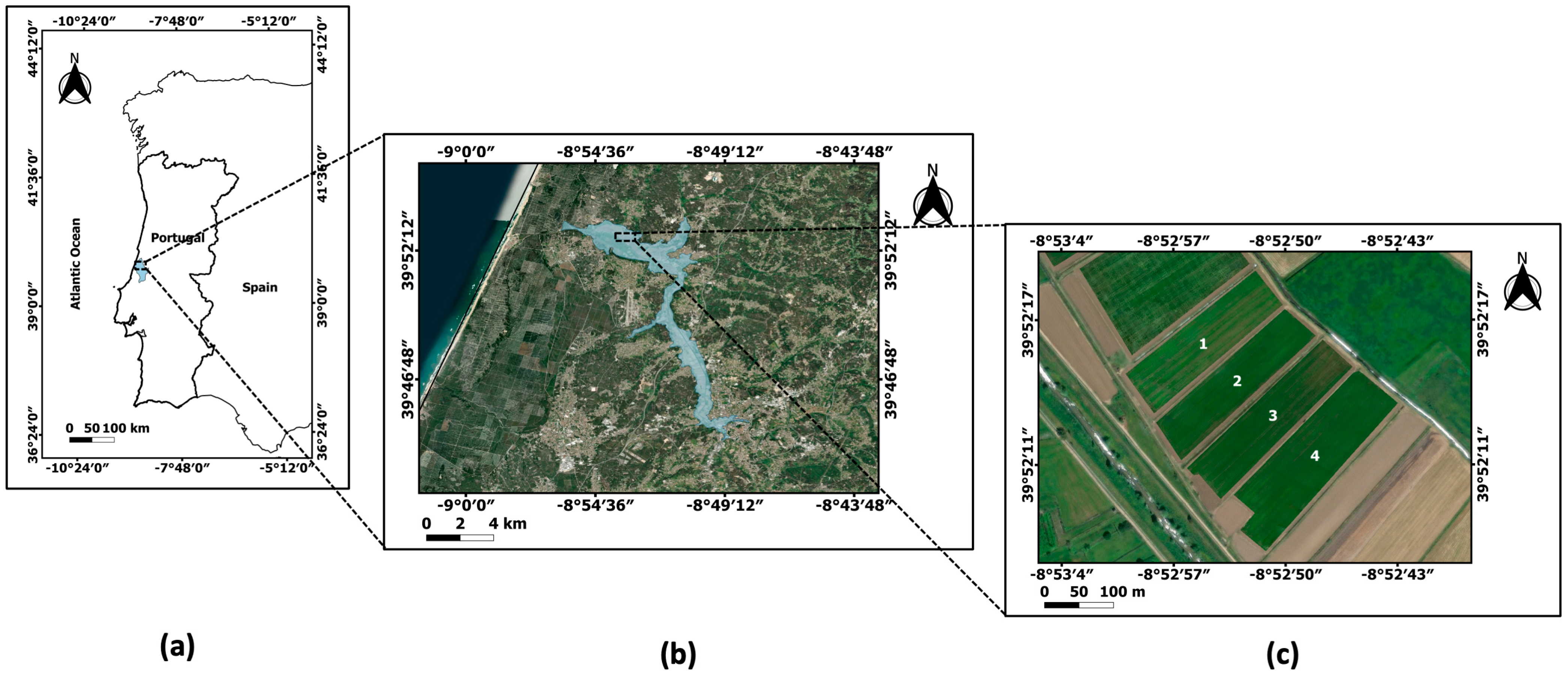
2.1. Study Area

This experimental study focused on rice cultivation in the Lis Valley Irrigation District (LVID) (Figure 1). LVID is a state initiative situated in the municipalities of Leiria and Marinha Grande, in the Center of Portugal, in proximity to the Atlantic Coast. It serves an agricultural area of about 2130 ha, with approximately 1490 ha of this area being irrigated. The main crops include forage corn, forage grass, horticultural crops, orchards, and rice, which is grown on an area of around 140 ha [38,39]. The rice produced has a long grain and belongs to the variety Ariete, subspecies Oryza sativa L. spp. japonica; commercially, it is known as “Carolino” rice.
According to the Köppen–Geiger climate classification, the climate in the study area is Csb. Summers are temperate with low precipitation, and winters are rainy with mild temperatures [40]. During the summer, the climate is primarily influenced by the Mediterranean Sea and characterized by high temperatures, sunshine, and very little precipitation. During the winter, the climate is influenced by the Atlantic Ocean, with most of the precipitation in this season originating from frontal systems [41]. The mean annual precipitation in the Lis catchment (≈850 km2) is around 855 mm, but it decreases from the headwaters of the catchment towards the coastal region. Annual precipitation occurs mostly from September to December [42,43].
The soils are predominantly of alluvial origin and have high agricultural value; however, in some areas, they are poorly drained, facing waterlogging and salinization risks, particularly in the downstream areas where rice is cultivated in traditional rice paddies.
On average, the rice crop season in this region is from May to October, when harvesting takes place. The crop season lasts approximately 140–150 days [44]; for this type of long cultivation cycle [45], the vegetative phase typically lasts between 75 and 85 days for direct-seeded rice. Direct wet seeding is applied, and the conventional irrigation practice is the continuous flooding of the rice fields. During the cultivation season, approximately two months after sowing, the rice plants reach maximum vigor (the plant growing peak occurs between July and August), which then gradually decreases until harvest time [46]. Regarding rice irrigation, crop fields are flooded at the time of sowing, and the flooding is typically interrupted 2–3 weeks before harvest. However, the depth of the water layer ponded on the soil surface varies during the rice cultivation period, depending on the crop growth stage and the irrigation practice [44].
For this study, which focused on data from 2020, four contiguous rice cultivation plots were selected (Figure 1c): plot 1, 1.86 ha; plot 2, 1.65 ha; plot 3, 1.79 ha; and plot 4, 2.34 ha (coordinates: 39°52′15.29″ N, 8°52′54.23″ W; altitude: ≈10 m a.s.l.). The plots were located on the right bank of the Lis River, in the downstream part of the LVID. In 2020, the agronomic practices in these plots were similar regarding sowing dates (mid-May) and the application of conventional practices [47], namely continuous flooding irrigation and agronomic practices such as fertilization and other field management decisions. The soil presented 7% sand, 37% silt and 56% clay, with an average root zone depth of approximately 40 cm [47].

2.2. UAS Data Acquisition and Processing

In this study, the presence and condition of the rice plants found in the selected cultivation plots (Section 2.1) were explored using UAS remote sensing-based products. The data were collected using a DJI Matrice 600 drone (DJI, Shenzhen, China) (Figure 2a) equipped with a 1.2-megapixel MicaSense Red Edge—M MS sensor (MicaSense, Inc., Seattle, WA, USA) (Figure 2b), with a resolution of 1280 × 960 pixels This MS sensor covered the following relevant spectral wavelength bands: Blue (center wavelength: 475 nm; bandwidth: 32 nm), Green (center wavelength: 560 nm; bandwidth: 27 nm), Red (center wavelength: 668 nm; bandwidth: 16 nm), Red-edge (center wavelength: 717 nm; bandwidth: 12 nm), and NIR (Near Infrared; center wavelength: 840 nm; bandwidth: 57 nm). Based on the information provided by the manufacturer, the lens focal length is 5.4 mm, with a 46 degree field of view.
Radiometric calibration of the MS camera prior to the flight was ensured by scanning the MicaSense Calibrated Reflectance Panel and using procedures recommended by the manufacturer. MicaSense cameras are considered particularly sensitive and useful for comparing VIs, as discussed below, since each of the five bands used to calculate the indices have a narrow MS bandwidth [48].
The data analyzed in this work were collected during a UAS flight conducted on 9 July 2020, under conditions of minimal wind (less than 1 m/s) and clear sky. The DJI Matrice 600 drone was operated autonomously, following a pre-set flight plan consisting of a simple grid with a 25 m distance between flight lines. The flight plan included 75% overlap and 70% sidelap. With the drone flying at a height of 110 m above the ground, a ground sample distance of approximately 8 cm/pixel was obtained. The drone’s speed was set to 7.5 m/s. The camera was pointed nadir.
Radiometric correction was performed using the Camera, Sun Irradiance and Sun Angle option, utilizing a downwelling light sensor unit, as well as a GPS/inertial measurement unit [49]. The MicaSense RedEdge—M GPS provided an accuracy in the range of 2 to 3 m horizontally [50]. The UAS image data, including orthorectification, atmospheric correction and the generation of the VIs maps, were processed using the commercial software package Pix4DFields (version 1.9) from Pix4D (Pix4D S.A., Prilly, Switzerland). Pix4D has helped improve the application of small UASs for mapping by providing a structure-from-motion software package. The correction method included in Pix4D has been found to be capable of generating reflectance maps of reasonable/good quality [51,52,53], although flight circumstances influence the performance of calibration methods.

2.3. Vegetation Indices Calculation

This study explored two classes of VIs calculated from RS data collected using a UAS: RGB and MS indices. The RGB VIs, obtained from the MicaSense RedEdge—M sensor observations, were the Visible Atmospherically Resistant Index (VARI) [54] and Triangular Greenness Index (TGI) [55]. VARI is used for estimating leaf coverage [56] and TGI was developed to monitor leaf chlorophyll (Chl) content [57]. Few studies compare the utilization of selected RGB indices with the most common spectral indices to prove their use for common agricultural rice application [58,59,60]. The selected MS VIs were the Normalized Difference Vegetation Index (NDVI) [61], Blue Normalized Difference Vegetation Index (BNDVI) [62], Green Normalized Difference Vegetation Index (GNDVI) [63], Normalized Difference Red-Edge (NDRE) [64] and Modified Chlorophyll Absorption in Reflectance Index 1 (MCARI1) [65]. All these MS VIs rely on the NIR band; when combined with other bands, they use the characteristic shape of the green vegetation spectrum by combining the low reflectance in the visible wavelengths with the high reflectance of the NIR wavelengths [48]. Among the selected MS indices, the NDVI is the most widely applied for assessing leaf coverage and plant health. In particular, the MCARI1 is used to estimate Chl concentration including variations in the Leaf Area Index.
The calculation of the pixels’ VIs values was provided by the Pix4D software [49], using the equations shown in Table 1. The TGI and MCARI1 equations in Table 1 are based on the models proposed by Hunt et al. (2011) [55] and Haboudane et al. (2004) [65], respectively; in particular, they are normalized to the maximum value of the reflectance in the used bands.
All the selected indices highlight the greenness with higher values. The normalized indices NDVI, BNDVI, GNDVI and NDRE take values in the interval [−1, +1]; positive values signal vegetation; and values approaching +1 indicate conditions of maximum plant vigor. Typically, values near zero reveal bare soil and negative values reveal water surfaces. For VARI and TGI, positive values signal the presence of greenness, whereas usually, VARI negative values indicate soil objects [66] and TGI negative values are associated with plants’ low Chl content [67].
In general, the interpretation of spectral indices’ signals needs to be conducted on a case-by-case basis [68,69,70].

2.4. Vegetation Indices Analysis

The analysis of the collected data on rice field conditions, which aimed to explore the capability of RGB VIs to monitor the rice crop in comparison to the most widely spread application of MS VIs for that same purpose, included the following approaches: (i) data obtained for the four selected plots were analyzed separately; (ii) basic descriptive statistics were obtained for the selected data, extracted using the zonal statistics plugin in QGIS software [71]; (iii) the empirical frequency distributions obtained for the VIs’ pixel data were investigated; (iv) cross-correlations between the seven VIs, which included five MS indices and two RGB indices, were studied based on 15% of the pixel data, randomly chosen, and the calculation of the Pearson correlation coefficient; and (v) linear relationships between the MS and RGB VIs were explored, and the statistical significance of the regression coefficients was evaluated using the t-test.

3. Results and Discussion

3.1. Rice Monitoring at the Field Plot Scale

Figure 3 shows NDVI, BNDVI, GNDVI, NDRE, MCARI1, VARI, and TGI (Figure 3a–g) maps of the selected rice plots, during the late vegetative phase of the crop (on average, 56 days after sowing, for an estimated vegetative phase of about 84 days). These maps were created from MS and visible bands’ data collected on 9 July 2020, using a UAS (Section 2.2). For all indices shown in Figure 3, a red, green, and yellow color palette was used. However, the maps are not directly comparable, as indicated by the legends, which show the correspondence between the colors and the indices’ values. It is important to note that (i) the range of values for the different indices is typically not the same; and (ii) MCARI1, VARI, and TGI are non-normalized indices and were not designed to take values in the interval [−1, +1] like NDVI, BNDVI, GNDVI and NDRE. In particular, TGI values spanned the narrowest value range.
The maps in Figure 3 reveal differences in the way the rice crop in each field is captured by each of the VIs. Since the data were collected during the late vegetative phase of the rice growth period, it could be expected that the presence of young, healthy rice exhibiting vigorous photosynthesis produced strong reflection in the NIR band and absorption in the visible wavelength bands [72]. This is expected to be more strongly indicated by the indices that reveal higher capability to identify the plants’ Chl content. However, it was noticed that the lower pixel values taken by the VIs at the field scale, which typically reveal the plants’ low vigor, are found in the rice fields’ areas/spots that present larger ground level variations, due to irregular land levelling. In this respect, ground-level differences are more pronounced in plots 3 and 4 and could reach about 0.60 m. The unevenness of the ground level within the fields was revealed by the topographic map produced from the field survey. Thus, the smaller depth of the ponded irrigation water in these sub-areas, in relation to the water depth established elsewhere by the irrigation of the fields, and the aerobic conditions that could likely affect these areas between water applications, might have negatively impacted the plants’ development, including their growth and vigor [73].

3.2. Basic Descriptive Statistics

Table 2 presents descriptive statistics for the UAS-based VIs’ pixel values calculated in this study for each rice plot. The BNDVI, NDVI and GNDVI exhibited the highest mean values in each plot. In particular, the magnitude of the BNDVI and NDVI was similar, with BNDVI attaining the largest values. While differences between the selected normalized VIs are expected, especially for rice [37], their magnitudes are not directly comparable with the mean values displayed by the non-normalized indices. For example, MCARI1, which had the lowest mean values among the MS indices in this case, was found suitable for estimating Chl content variation by Zhang et al. (2021) [74]. They noted that, in the rice vegetative phase, the leaf Chl content within the rice canopy is higher in the lower leaves situated near the soil surface than in the upper leaves, and that such a fact could be well captured by this index.
Regarding the detection of heterogeneity at the field scale, particularly through the assessment of dispersion in the pixel datasets, it was the MCARI1 that revealed the highest coefficient of variation (CV) values among the MS indices (Table 2), ranging from 0.16 to 0.26. However, it was VARI (an RGB index) that even exhibited the highest CV values (ranging from 0.19 to 0.36) compared to the MCARI1 CVs, for all plots. This suggests that VARI has a strong capability to respond to the lack of homogeneity in the rice fields. The mean values of VARI fell between those of GNDVI and NDRE, which were higher than the values calculated for NDVI and BNDVI. BNDVI, on the other hand, presented the lowest CV values (ranging from 0.04 to 0.07), indicating that this index might have the lowest ability to identify variations in rice growing conditions at the field scale among the selected indices, at least in this growing phase. Generally, the normalized MS indices had CV values lower than 15%. As for the other RGB index, TGI exhibited a CV higher than the CV calculated for the MS indices, except MCARI1. However, this difference in CV values could be influenced by the relative lower magnitude of TGI compared to the other indices, as CV values tend to be high at very low values and low at high values.
It is worth noting that the target of the two RGB indices, VARI and TGI, is different. VARI was developed to monitor the fractional area covered by vegetation [75], whereas TGI was developed to monitor leaf Chl content [76]. Particularly, in terms of within-field variations, TGI behaved similarly to MCARI1 (e.g., [55]), despite the different spectral bands involved in their calculation, although the CV values calculated for MCARI1 were somewhat higher. This difference in CV values was consistently maintained for all four plots.
Overall, plot 4 consistently showed the lowest CV values for all the indices, while plots 1 and 3 consistently exhibited the highest CV values. Plot 4 also had the highest mean values for all selected indices (both MS and RGB indices) among the four plots.

3.3. Empirical Frequency Distributions of Pixel-Value Data

The empirical frequency distributions of the VIs’ pixel data were inspected. Histograms for selected MS and RGB VIs are displayed in Figure 4 (NDVI and VARI) and Figure 5 (MCARI1 and TGI) for the four field plots, with sample sizes provided in Table 2. These histograms reveal differences in the magnitude and value–range of these indices, which are not directly comparable due to their distinct formulation. However, Figure 4 and Figure 5 demonstrate similarities and disparities in the shapes of the frequency distributions for these MS and RGB VIs pixel values within each field plot, offering a more comprehensive understanding of the data beyond just the mean values.
In Figure 6, box and whisker plots are presented for the empirical frequency distributions of MS VI (NDVI and MCARI1) and RGB VI (VARI and TGI) pixel values. These plots show the mean, median, lower and upper quartiles, and range of the distributions, providing a clearer depiction of central tendencies as well as information about the dispersion around these central values for the four rice plots. This approach offers a more detailed view of the data’s characteristics compared to examining means alone.
The box and whisker plots presented in Figure 6 highlight several observations in comparison to NDVI, which is typically regarded as a good indicator of the fraction and status of the vegetation within rice plots: (i) the VARI index suggests greater within-field variation, although it is important to note that this comparison involves a normalized and a non-normalized index; (ii) the response signals of MCARI1 and TGI indicate that their ability to detect small differences in leaf Chl content is comparable, and their performance relative to NDVI appears to be superior, despite their narrower value ranges compared to NDVI. However, in this comparison between the response signals of MS and RGB indices, what is most relevant is the consistency in their behavior, which is suggested by the results in this case. Further discussions on the relationships between selected indices are provided below.

3.4. Cross-Correlation Analysis

Figure 7 shows the cross-correlation coefficients (i.e., Pearson correlation coefficients, denoted as “r”) for the selected VIs in relation to each of the studied rice plots during the late vegetative phase of rice growth. Given that NDVI is the most commonly used and well-known vegetation index, it is of particular interest to understand how this index correlates with the other VIs used in this study. The analysis revealed that the correlation between NDVI and the other MS VIs was very strong, with an average correlation coefficient of r = 0.92 ± 0.05. This was especially true for BNDVI and GNDVI, which showed extremely high correlations (r = 0.97 ± 0.02 and 0.94 ± 0.03, respectively). Such strong correlations have also been reported by other authors (e.g., [29]). Among the normalized indices, NDRE exhibited a stronger correlation with GNDVI (r = 0.95 ± 0.02) than with NDVI (r = 0.85 ± 0.05) or BNDVI (r = 0.84 ± 0.06).
Regarding the two RGB VIs, the results indicated a very strong correlation between NDVI and VARI (r = 0.97 ± 0.01), and a strong correlation between NDVI and TGI (r = 0.75 ± 0.09). The correlation between BNDVI and VARI (r = 0.90 ± 0.05) was stronger than between GNDVI and VARI (r = 0.85 ± 0.07), but weaker than between NDVI and VARI. Additionally, the correlation between NDRE and VARI (r = 0.77 ± 0.09) was stronger than that between NDRE and TGI (r = 0.47 ± 0.16). Notably, a strong correlation was observed between MCARI1 and VARI (r = 0.90 ± 0.06) as well as between MCARI1 and TGI (r = 0.88 ± 0.03), which is consistent with findings from previous studies [76,77], although those studies were not specific for rice.
The analysis also revealed that the RS signal captured for plot 4 differed from the signal captured for the other three plots, resulting in consistently higher mean values for the VIs and lower Pearson correlation coefficients in the cross-correlation analysis for all indices. While this could suggest that the rice development in plot 4 was more advanced compared to the other plots, it was not possible to confirm this with independent data.

3.5. MS and RGB Indices Relationships

The previous section highlighted the presence of positive relationships between MS and RGB VIs. Furthermore, the RGB VIs exhibited strong correlations with MS VIs (Figure 7), especially with NDVI, BNDVI and MCARI1, with the correlation being more robust for VARI compared to TGI. Additionally, the data collected on 9 July 2020 indicated that linear models could describe the relationship between MS VIs and RGB VIs under the surveyed conditions. Figure 8 and Figure 9 illustrate the data, their positive relationships, the corresponding linear models and the coefficients of determination for the relationship between NDVI and VARI, as well as between MCARI1 and TGI. All results are statistically significant (p-value < 0.001). A cursory assessment of these correlations would classify them as very strong in the first case (NDVI and VARI) and strong in the other case (MCARI1 and TGI).
The results suggest that the RGB indices VARI and TGI, calculated from data collected via a cost-effective aerial drone equipped with a RGB camera, can provide valuable information at high-spatial resolution regarding the rice crop conditions at the field scale. This preliminary assessment is based on the observed relationships between these indices and several MS VIs, including the widely used NDVI. These findings indicate the feasibility of utilizing real-image cameras (RGB cameras) as a cost-effective alternative to MS cameras for monitoring rice paddies, using RGB VIs as tools that could enhance paddy fields management. This conclusion is drawn from data collected during the late vegetative stage of the rice cultivation cycle, and further investigation is needed to assess other rice development stages and growth conditions for a more comprehensive understanding. To strengthen the utility of RGB indices for rice crop monitoring, it would be beneficial to acquire data related to growth parameters such as biomass, nitrogen content, or chlorophyll content. Additionally, when selecting a VI, considerations should also encompass (i) the specific parameter to be estimated, (ii) the expected range of this parameter, and (iii) prior knowledge of the variations in external factors affecting the spectral reflectance of the canopy [76].

4. Conclusions

Whereas the literature reveals many studies employing UAS-based MS VIs in rice farming, the use of RGB VIs has been poorly explored, and studies dedicated to rice farming in Europe, namely in the Mediterranean area, are also scarce. This study explores UAS-based RGB imagery of rice fields with a focus on the crop status and on this geographical region.
The main outcomes of this study are:
(i).
High-resolution UAS sensors and photogrammetric techniques that are commonly applied to collect MS imagery have the capability to generate data for creating VIs’ maps that provide useful information for agriculture, namely for rice farming.
(ii).
RGB VIs, namely VARI and TGI, which can be calculated from visible RGB bands only, could provide valuable assistance for monitoring and managing rice field plots.
(iii).
The access to VIs’ mapping of rice fields (such as VARI and TGI mapping) through the use of digital cameras mounted on UASs, which are able to collect RS imagery at a lower cost than MS cameras, may constitute an opportunity to a larger number of farmers to use RS products to monitor paddy fields in a quick and cost-effective manner and, therefore, improve rice crop management, towards an increasingly sustainable rice agriculture and protection of the environment.
Overall, similarly to other studies, this study confirmed that UAS technology and the MS and RGB imagery and products that it provides could be suitable and convenient tools for agricultural monitoring. The main contribution of this study is that it is focused on the rice crop at the field scale, whereas only a few studies evaluated RGB indices for rice growth management; thus, it improves the viability of paddy precision farming through the use of low-cost sensors, namely in Mediterranean areas, but also in other soil, climatic and hydrologic conditions. However, suitable technical knowledge and local support should be provided to farmers to guarantee that the implementation of these technologies is meaningful, so that production is optimized for better profitability and environmental sustainability is pursued. Further studies are needed that embrace a wider range of field and rice crop growth stage conditions, namely field surveys for validation of the spectral signal and information obtained at different stages of the rice cultivation cycle. The impact of the spatial resolution of the data needs to be assessed. These studies would provide better insight regarding the UAS flight conditions and cameras used, and the usefulness of UAS-based VARI, TGI and other RGB VIs for assessing rice cultivation conditions, in general.

Author Contributions

Conceptualization, R.G. and I.P.d.L.; methodology, R.G. and I.P.d.L.; formal analysis, R.G and I.P.d.L.; writing—original draft preparation, R.G. and I.P.d.L.; writing—review and editing, R.G. and I.P.d.L.; funding acquisition, I.P.d.L. All authors have read and agreed to the published version of the manuscript.

Funding

The research presented here was partly funded through the Portuguese Fundação para a Ciência e a Tecnologia (FCT), involving: project MEDWATERICE (PRIMA/0006/2018; with the support of PRIMA Programme), supported by national funds (PIDDAC); projects UIDB/04292/2020 and UIDP/04292/2020 granted to MARE—Marine and Environmental Research Center, and project LA/P/0069/2020 granted to the Associate Laboratory ARNET–Aquatic Research Network, supported by national funds.

Institutional Review Board Statement

Not applicable.

Data Availability Statement

The original contributions presented in the study are included in the article; further inquiries can be directed to the corresponding author.

Conflicts of Interest

The authors declare no conflict of interest.

References

  1. Cantrell, R.P.; Reeves, T.G. The Rice Genome: The Cereal of the World’s Poor Takes Center Stage. Science 2002, 296, 53. [Google Scholar] [CrossRef] [PubMed]
  2. Fageria, N.K. Plant tissue test for determination of optimum concentration and uptake of nitrogen at different growth stages in lowland rice. Commun. Soil Sci. Plant Anal. 2003, 34, 259–270. [Google Scholar] [CrossRef]
  3. Arellano, C.A.; Reyes, J.A.D. Effects of farmer-entrepreneurial competencies on the level of production and technical efficiency of rice farms in Laguna, Philippines. J. Int. Soc. Southeast Asian Agric. Sci. 2019, 25, 45–57. Available online: http://issaasphil.org/wp-content/uploads/2019/11/5.-Arellano_Delos-Reyes-2019-entrepreneurial_competencies-FINAL.pdf (accessed on 17 November 2022).
  4. Wang, L.; Liu, J.; Yang, L.; Chen, Z.; Wang, X.; Ouyang, B. Applications of unmanned aerial vehicle images on agricultural remote sensing monitoring. Trans. Chin. Soc. Agric. Eng. 2013, 29, 136–145. [Google Scholar] [CrossRef]
  5. Zhang, H.; Wang, L.; Tian, T.; Yin, J. A Review of unmanned aerial vehicle low-altitude remote sensing (UAV-LARS) use in agricultural monitoring in China. Remote Sens. 2021, 13, 1221. [Google Scholar] [CrossRef]
  6. Elmetwalli, A.H.; Mazrou, Y.S.A.; Tyler, A.N.; Hunter, P.D.; Elsherbiny, O.; Yaseen, Z.M.; Elsayed, S. Assessing the efficiency of remote sensing and machine learning algorithms to quantify wheat characteristics in the Nile Delta region of Egypt. Agriculture 2022, 12, 332. [Google Scholar] [CrossRef]
  7. San Bautista, A.; Fita, D.; Franch, B.; Castiñeira-Ibáñez, S.; Arizo, P.; Sánchez-Torres, M.J.; Becker-Reshef, I.; Uris, A.; Rubio, C. Crop Monitoring Strategy Based on Remote Sensing Data (Sentinel-2 and Planet), Study Case in a Rice Field after Applying Glycinebetaine. Agronomy 2022, 12, 708. [Google Scholar] [CrossRef]
  8. Tucker, C.J. Remote sensing of leaf water content in the near infrared. Remote Sens. Environ. 1980, 10, 23–32. [Google Scholar] [CrossRef]
  9. Pan, Z.; Huang, J.; Zhou, Q.; Wang, L.; Cheng, Y.; Zhang, H.; Blackburn, G.A.; Yan, J.; Liu, J. Mapping crop phenology using NDVI time-series derived from HJ-1 A/B data. Int. J. Appl. Earth Obs. Geoinf. 2015, 34, 188–197. [Google Scholar] [CrossRef]
  10. Van Niel, T.G.; McVicar, T.R. Current and potential uses of optical remote sensing in rice-based irrigation systems: A review. Aust. J. Agric. Res. 2004, 55, 155–185. [Google Scholar] [CrossRef]
  11. Hively, W.; Lang, M.; McCarty, G.; Keppler, J.; Sadeghi, A.; McConnell, L. Using satellite remote sensing to estimate winter cover crop nutrient uptake efficiency. J. Soil Water Conserv. 2009, 64, 303–313. [Google Scholar] [CrossRef]
  12. Zulfa, A.W.; Norizah, K. Remotely sensed imagery data application in mangrove forest: A review. Pertanika J. Sci. Technol. 2018, 26, 899–922. Available online: http://www.pertanika.upm.edu.my/pjtas/browse/regular-issue?article=JST-0904-2017 (accessed on 10 May 2023).
  13. Ren, H.; Zhou, G.; Zhang, F. Using Negative Soil Adjustment Factor in Soil-Adjusted Vegetation Index (SAVI) for Aboveground Living Biomass Estimation in Arid Grasslands. Remote Sens. Environ. 2018, 209, 439–445. [Google Scholar] [CrossRef]
  14. Manfreda, S.; McCabe, M.; Miller, P.; Lucas, R.; Pajuelo Madrigal, V.; Mallinis, G.; Ben Dor, E.; Helman, D.; Estes, L.; Ciraolo, G.; et al. On the Use of Unmanned Aerial Systems for Environmental Monitoring. Remote Sens. 2018, 10, 641. [Google Scholar] [CrossRef]
  15. Huang, Y.; Thomson, S.J.; Hoffmann, W.C.; Lan, Y.; Fritz, B.K. Development and Prospect of Unmanned Aerial Vehicle Technologies for Agricultural Production Management. Int. J. Agric. Biol. Eng. 2013, 6, 11. Available online: https://ijabe.org/index.php/ijabe/article/view/900/0 (accessed on 28 April 2023).
  16. Li, C.; Li, H.; Li, J.; Lei, Y.; Li, C.; Manevski, K.; Shen, Y. Using NDVI Percentiles to Monitor Real-Time Crop Growth. Comput. Electron. Agric. 2019, 162, 357–363. [Google Scholar] [CrossRef]
  17. Abdullah, S.; Tahar, K.N.; Rashid, M.F.A.; Osoman, M.A. Camera calibration performance on different non-metric cameras. Pertanika J. Sci. Technol. 2019, 27, 1397–1406. Available online: http://www.pertanika2.upm.edu.my/resources/files/Pertanika%20PAPERS/JST%20Vol.%2027%20%20Jul.%202019/25%20JST-1183-2018.pdf (accessed on 4 May 2023).
  18. Pinguet, B. The Role of Drone Technology in Sustainable Agriculture. Available online: https://www.precisionag.com/in-field-technologies/drones-uavs/the-role-of-drone-technology-in-sustainable-agriculture/ (accessed on 4 May 2023).
  19. Singh, K.K.; Frazier, A.E. A meta-analysis and review of unmanned aircraft system (UAS) imagery for terrestrial applications. Int. J. Remote Sens. 2018, 39, 5078–5098. [Google Scholar] [CrossRef]
  20. Maes, W.H.; Steppe, K. Perspectives for remote sensing with unmanned aerial vehicles in precision agriculture. Trends Plant Sci. 2019, 24, 152–164. [Google Scholar] [CrossRef] [PubMed]
  21. Cen, H.; Wan, L.; Zhu, J.; Li, Y.; Li, X.; Zhu, Y.; Weng, H.; Wu, W.; Yin, W.; Xu, C.; et al. Dynamic monitoring of biomass of rice under different nitrogen treatments using a lightweight UAV with dual image-frame snapshot cameras. Plant Methods 2019, 15, 32. [Google Scholar] [CrossRef] [PubMed]
  22. Zhou, J.; Wang, B.W.; Fan, J.H.; Ma, Y.C.; Wang, Y.; Zhang, Z. A Systematic Study of Estimating Potato N Concentrations Us-ing UAV-Based Hyper- and Multi-Spectral Imagery. Agronomy 2022, 12, 2533. [Google Scholar] [CrossRef]
  23. Pádua, L.; Matese, A.; Gennaro, S.F.D.; Morais, R.; Peres, E.; Sousa, J.J. Vineyard classification using OBIA on UAV-based RGB and multispectral data: A case study in different wine regions. Comput. Electron. Agric. 2022, 196, 106905. [Google Scholar] [CrossRef]
  24. Schirrmann, M.; Giebel, A.; Gleiniger, F.; Pflanz, M.; Lentschke, J.; Dammer, K.H. Monitoring agronomic parameters of winter wheat crops with low-cost UAV imagery. Remote Sens. 2016, 8, 706. [Google Scholar] [CrossRef]
  25. Singh, K.D.; Starnes, R.; Kluepfel, D.; Nansen, C. Qualitative analysis of walnut trees rootstock using airborne remote sensing. In Proceedings of the Sixth Annual Plant Science Symposium, UC Davis, CA, USA, 31 January 2017. [Google Scholar]
  26. Hasan, U.; Sawut, M.; Chen, S. Estimating the Leaf Area Index of Winter Wheat Based on Unmanned Aerial Vehicle RGB-Image Parameters. Sustainability 2019, 11, 6829. [Google Scholar] [CrossRef]
  27. Andrade, R.G.; Hott, M.C.; Magalhães Junior, W.C.P.D.; D’Oliveira, P.S. Monitoring of Corn Growth Stages by UAV Platform Sensors. Int. J. Adv. Eng. Res. Sci. 2019, 6, 54–58. [Google Scholar] [CrossRef]
  28. Choroś, T.; Oberski, T.; Kogut, T. UAV Imaging at RGB for Crop Condition Monitoring. Int. Arch. Photogramm. Remote Sens. Spatial Inf. Sci. 2020, 43, 1521–1525. [Google Scholar] [CrossRef]
  29. García-Martínez, H.; Flores, H.; Ascencio-Hernández, R.; Khalil-Gardezi, A.; Tijerina-Chávez, L.; Mancilla-Villa, O.R.; Vázquez-Peña, M.A. Corn Grain Yield Estimation from Vegetation Indices, Canopy Cover, Plant Density, and a Neural Network Using Multispectral and RGB Images Acquired with Unmanned Aerial Vehicles. Agriculture 2020, 10, 277. [Google Scholar] [CrossRef]
  30. Singh, A.P.; Yerudkar, A.; Mariani, V.; Iannelli, L.; Glielmo, L. A Bibliometric Review of the Use of Unmanned Aerial Vehicles in Precision Agriculture and Precision Viticulture for Sensing Applications. Remote Sens. 2022, 14, 1604. [Google Scholar] [CrossRef]
  31. Cheng, M.; Jiao, X.; Liu, Y.; Shao, M.; Yu, X.; Bai, Y.; Wang, Z.; Wang, S.; Tuohuti, N.; Liu, S.; et al. Estimation of soil moisture content under high maize canopy coverage from UAV multimodal data and machine learning. Agric. Water Manag. 2022, 264, 107530. [Google Scholar] [CrossRef]
  32. Ge, H.; Xiang, H.; Ma, F.; Li, Z.; Qiu, Z.; Tan, Z.; Du, C. Estimating Plant Nitrogen Concentration of Rice through Fusing Vegetation Indices and Color Moments Derived from UAV-RGB Images. Remote Sens. 2021, 13, 1620. [Google Scholar] [CrossRef]
  33. Dimyati, M.; Supriatna, S.; Nagasawa, R.; Pamungkas, F.D.; Pramayuda, R. A Comparison of Several UAV-Based Multispectral Imageries in Monitoring Rice Paddy (A Case Study in Paddy Fields in Tottori Prefecture, Japan). IJGI 2023, 12, 36. [Google Scholar] [CrossRef]
  34. Kazemi, F.; Ghanbari Parmehr, E. Evaluation of RGB Vegetation Indices Derived from UAV Images for Rice Crop Growth Monitoring. ISPRS Ann. Photogramm. Remote Sens. Spat. Inf. Sci. 2023, 10, 385–390. [Google Scholar] [CrossRef]
  35. Ristorto, G.; Mazzetto, F.; Guglieri, G.; Quagliotti, F. Monitoring performances and cost estimation of multirotor Unmanned Aerial Systems in precision farming. Int. Conf. Unmanned Aircr. Syst. 2015, 7152329, 502–509. [Google Scholar] [CrossRef]
  36. Stroppiana, D.; Villa, P.; Sona, G.; Ronchetti, G.; Candiani, G.; Pepe, M.; Busetto, L.; Migliazzi, M.; Boschetti, M. Early season weed mapping in rice crops using multi-spectral UAV data. Int. J. Remote Sens. 2018, 39, 5432–5452. [Google Scholar] [CrossRef]
  37. de Lima, I.P.; Jorge, R.G.; de Lima, J.L.M.P. Remote Sensing Monitoring of Rice Fields: Towards Assessing Water Saving Irrigation Management Practices. Front. Remote Sens. 2021, 2, 762093. [Google Scholar] [CrossRef]
  38. Gonçalves, J.M.; Ferreira, S.; Nunes, M.; Eugénio, R.; Amador, A.; Filipe, O.; Duarte, I.M.; Teixeira, M.; Vasconcelos, T.; Oliveira, F.; et al. Developing Irrigation Management at District Scale Based on Water Monitoring: Study on Lis Valley, Portugal. Agric. Eng. 2020, 2, 78–95. [Google Scholar] [CrossRef]
  39. USDA. Portuguese Rice Imports Pick up as Production Declines—USDA Gain Report; USDA: Washington, DC, USA, 2017; p. 13. [Google Scholar]
  40. IPMA. IPMA Home Page. Available online: https://www.ipma.pt (accessed on 10 November 2022).
  41. Mora, C.; Vieira, G. The Climate of Portugal. In Landscapes and Landforms of Portugal; Vieira, G., Zêzere, J.L., Mora, C., Eds.; Springer International Publishing: Cham, Switzerland, 2020; pp. 33–46. ISBN 978-3-319-03641-0. [Google Scholar] [CrossRef]
  42. SNIRH. SNIRH Home Page. Available online: https://snirh.apambiente.pt/ (accessed on 1 December 2022).
  43. Fonseca, A.; Botelho, C.; Boaventura, R.A.R.; Vilar, V.J.P. Integrated hydrological and water quality model for river management: A case study on Lena River. Sci. Total Environ. 2014, 485–486, 474–489. [Google Scholar] [CrossRef] [PubMed]
  44. Gonçalves, J.M.; Nunes, M.; Jordão, A.; Ferreira, S.; Eugénio, R.; Bigeriego, J.; Duarte, I.; Amador, P.; Filipe, O.; Damásio, H.; et al. The Challenges of Water Saving in Rice Irrigation: Field Assessment of Alternate Wetting and Drying Flooding and Drip Irrigation Techniques in the Lis Valley, Portugal. In Proceedings of the 1st International Conference on Water Energy Food and Sustainability (ICoWEFS 2021), Leiria, Portugal, 10–12 May 2021; Springer: Cham, Switzerland, 2021. [Google Scholar] [CrossRef]
  45. Rice Knowledge Bank. Rice Knowledge Bank Home Page. Available online: http://www.knowledgebank.irri.org/step-by-step-production/pre-planting/crop-calendar (accessed on 10 December 2022).
  46. de Lima, I.P.; Jorge, R.G.; de Lima, J.L.M.P. Aplicação de Técnicas de Deteção Remota na Avaliação da Cultura do Arroz. In Proceedings of the 15° Congresso da Água, Lisboa, Portugal, 22–26 March 2021; Available online: https://www.aprh.pt/congressoagua2021/docs/15ca_142.pdf (accessed on 14 January 2023).
  47. Ferreira, S.; Sánchez, J.M.; Gonçalves, J.M. A Remote-Sensing-Assisted Estimation of Water Use in Rice Paddy Fields: A Study on Lis Valley, Portugal. Agronomy 2023, 13, 1357. [Google Scholar] [CrossRef]
  48. Daughtry, C.S.; Walthall, C.; Kim, M.; De Colstoun, E.B.; McMurtrey Iii, J. Estimating corn leaf chlorophyll concentration from leaf and canopy reflectance. Remote Sens. Environ. 2000, 74, 229–239. [Google Scholar] [CrossRef]
  49. Pix4Dmapper 4.1 User Manual. Available online: https://support.pix4d.com/hc/en-us/articles/204272989-Offline-Getting-Started-and-Manual-pdf (accessed on 21 July 2023).
  50. Avtar, R.; Suab, S.A.; Syukur, M.S.; Korom, A.; Umarhadi, D.A.; Yunus, A.P. Assessing the influence of UAV altitude on extracted biophysical parameters of young oil palm. Remote Sens. 2020, 12, 3030. [Google Scholar] [CrossRef]
  51. Cubero-Castan, M.; Schneider-Zapp, K.; Bellomo, M.; Shi, D.; Rehak, M.; Strecha, C. Assessment of the Radiometric Accuracy in A Target Less Work Flow Using Pix4D Software. In Proceedings of the Workshop on Hyperspectral Image and Signal Processing, Evolution in Remote Sensing, Amsterdam, The Netherlands, 23–26 September 2018. [Google Scholar] [CrossRef]
  52. Qin, Z.; Li, X.; Gu, Y. An Illumination Estimation and Compensation Method for Radiometric Correction of UAV Multispectral Images. IEEE Trans. Geosci. Remote Sens. 2022, 60, 5545012. [Google Scholar] [CrossRef]
  53. Daniels, L.; Eeckhout, E.; Wieme, J.; Dejaegher, Y.; Audenaert, K.; Maes, W.H. Identifying the Optimal Radiometric Calibration Method for UAV-Based Multispectral Imaging. Remote Sens. 2023, 15, 2909. [Google Scholar] [CrossRef]
  54. Gitelson, A.; Merzlyak, M.N. Spectral Reflectance Changes Associated with Autumn Senescence of Aesculus hippocastanum L. and Acer platanoides L. Leaves. Spectral Features and Relation to Chlorophyll Estimation. J. Plant Physiol. 1994, 143, 286–292. [Google Scholar] [CrossRef]
  55. Hunt, E.R.; Daughtry, C.S.T.; Eitel, J.U.; Long, D.S. Remote Sensing Leaf Chlorophyll Content Using a Visible Band Index. Agron. J. 2011, 103, 1090–1099. [Google Scholar] [CrossRef]
  56. Gitelson, A.A.; Stark, R.; Grits, U.; Rundquist, D.; Kaufman, Y.; Derry, D. Vegetation and soil lines in visible spectral space: A concept and technique for remote estimation of vegetation fraction. Int. J. Remote Sens. 2002, 23, 2537–2562. [Google Scholar] [CrossRef]
  57. Hunt, E.R., Jr.; Doraiswamy, P.C.; McMurtrey, J.E.; Daughtry, C.S.; Perry, E.M.; Akhmedov, B. A visible band index for remote sensing leaf chlorophyll content at the canopy scale. Int. J. Appl. Earth Obs. Geoinf. 2013, 21, 103–112. [Google Scholar] [CrossRef]
  58. Wan, L.; Cen, H.; Zhu, J.; Zhang, J.; Zhu, Y.; Sun, D.; Du, X.; Zhai, L.; Weng, H.; Li, Y.; et al. Grain yield prediction of rice using multi-temporal UAV-based RGB and multispectral images and model transfer—A case study of small farmlands in the South of China. Agric. For. Meteorol. 2020, 291, 108096. [Google Scholar] [CrossRef]
  59. Zhou, X.; Zheng, H.B.; Xu, X.Q.; He, J.Y.; Ge, X.K.; Yao, X.; Cheng, T.; Zhu, Y.; Cao, W.X.; Tian, Y.C. Predicting grain yield in rice using multi-temporal vegetation indices from UAV-based multispectral and digital imagery. ISPRS J. Photogramm. 2017, 130, 246–255. [Google Scholar] [CrossRef]
  60. Wójcik-Gront, E.; Gozdowski, D.; Stępień, W. UAV-Derived Spectral Indices for the Evaluation of the Condition of Rye in Long-Term Field Experiments. Agriculture 2022, 12, 1671. [Google Scholar] [CrossRef]
  61. Rouse, J.; Haas, R.; Schell, J.; Deering, D. Monitoring Vegetation Systems in the Great Plains with ERTS. In Proceedings of the Third ERTS (Earth Resources Technology Satellite) Symposium, NASA SP-351, Washington, DC, USA, 10–14 December 1973; NASA: Washington, DC, USA, 1973; Volume 1, pp. 309–317. [Google Scholar]
  62. Yang, C.; Everitt, J.H.; Bradford, J.M.; Murden, D. Airborne Hyperspectral Imagery and Yield Monitor Data for Mapping Cotton Yield Variability. Precis. Agric. 2004, 5, 445–461. [Google Scholar] [CrossRef]
  63. Gitelson, A.; Kaufman, Y.; Merzlyak, M. Use of a Green Channel in Remote Sensing of Global Vegetation from EOS-MODIS. Remote Sens. Environ. 1996, 58, 289–298. [Google Scholar] [CrossRef]
  64. Gitelson, A.; Merzlyak, M.N. Quantitative Estimation of Chlorophyll-a Using Reflectance Spectra: Experiments with Autumn Chestnut and Maple Leaves. J. Photochem. Photobiol. B Biol. 1994, 22, 247–252. [Google Scholar] [CrossRef]
  65. Haboudane, D.; Miller, J.R.; Pattey, E.; Zarco-Tejada, P.J.; Strachan, I.B. Hyperspectral vegetation indices and novel algorithms for predicting green LAI of crop canopies: Modeling and validation in the context of precision agriculture. Remote Sens. Environ. 2004, 90, 337–352. [Google Scholar] [CrossRef]
  66. Suud, H.M. An image processing approach for monitoring soil plowing based on drone RGB images. BDA 2022, 5, 1–5. [Google Scholar]
  67. Sedlar, A.; Gvozdenac, S.; Pejović, M.; Višacki, V.; Turan, J.; Tanasković, S.; Burg, P.; Vasić, F. The Influence of Wetting Agent and Type of Nozzle on Copper Hydroxide Deposit on Sugar Beet Leaves (Beta vulgaris L.). Appl. Sci. 2022, 12, 2911. [Google Scholar] [CrossRef]
  68. Ryu, J.-H.; Jeong, H.; Cho, J. Performances of Vegetation Indices on Paddy Rice at Elevated Air Temperature, Heat Stress, and Herbicide Damage. Remote Sens. 2020, 12, 2654. [Google Scholar] [CrossRef]
  69. Taylor-Zavala, R.; Ramírez-Rodríguez, O.; de Armas-Ricard, M.; Sanhueza, H.; Higueras-Fredes, F.; Mattar, C. Quantifying Biochemical Traits over the Patagonian Sub-Antarctic Forests and Their Relation to Multispectral Vegetation Indices. Remote Sens. 2021, 13, 4232. [Google Scholar] [CrossRef]
  70. Gerardo, R.; de Lima, I. Comparing the capability of Sentinel-2 and Landsat 9 imagery for mapping water and sandbars in the river bed of the Lower Tagus River (Portugal). Remote Sens. 2023, 15, 1927. [Google Scholar] [CrossRef]
  71. QGIS. 2023. QGIS Project. Available online: http://www.qgis.org/ (accessed on 10 March 2022).
  72. Boiarskii, B. Comparison of NDVI and NDRE Indices to Detect Differences in Vegetation and Chlorophyll Content. J. Mech. Contin. Math. Sci. 2019, 4, 20–29. [Google Scholar] [CrossRef]
  73. Miniotti, E.; Romani, M.; Said-Pullicino, D.; Facchi, A.; Bertora, C.; Peyron, M.; Sacco, D.; Bischetti, G.; Lerda, C.; Tenni, D.; et al. Agro-environmental sustainability of different water management practices in temperate rice agro-ecosystems. Agric. Ecosyst. Environ. 2016, 222, 235–248. [Google Scholar] [CrossRef]
  74. Zhang, J.; Wan, L.; Igathinathane, C.; Zhang, Z.; Guo, Y.; Sun, D.; Cen, H. Spatiotemporal Heterogeneity of Chlorophyll Content and Fluorescence Response Within Rice (Oryza sativa L.) Canopies Under Different Nitrogen Treatments. Front. Plant Sci. 2021, 12, 645977. [Google Scholar] [CrossRef] [PubMed]
  75. Gitelson, A.A.; Kaufman, Y.J.; Stark, R.; Rundquist, D. Novel algorithms for remote estimation of vegetation fraction. Remote Sens. Environ. 2002, 80, 76–87. [Google Scholar] [CrossRef]
  76. Broge, N.H.; Leblanc, E. Comparing prediction power and stability of broadband and hyperspectral vegetation indices for estimation of green leaf area index and canopy chlorophyll density. Remote Sens. Environ. 2001, 76, 156–172. [Google Scholar] [CrossRef]
  77. Jelínek, Z.; Mašek, J.; Starỳ, K.; Lukáš, J.; Kumhálová, J. Winter wheat, Winter Rape and Poppy Crop Growth Evaluation with the Help of Remote and Proximal Sensing Measurements. Agron. Res. 2020, 18, 2049–2059. [Google Scholar]
Figure 1. Study Area: (a) Location of the study area, in the Center of Portugal, near the Atlantic coast: the shaded blue identifies de Lis River catchment; (b) Location of the Lis Valley Irrigation District, LVID; (c) Location of the four selected rice fields in the LVID.
Agriculture 13 01916 g001
Figure 2. Unmanned Aerial System used in this experimental study: (a) DJI Matrice 600 drone and (b) MicaSense RedEdge—M multispectral sensor.
Agriculture 13 01916 g002
Figure 3. Maps of (a) NDVI, (b) BNDVI, (c) GNDVI, (d) NDRE, (e) MCARI1, (f) VARI and (g) TGI, for the selected rice plots (plots 1, 2, 3 and 4) in LVID.
Agriculture 13 01916 g003
Figure 4. Histograms of the pixels’ vegetation indices NDVI and VARI, respectively, for the selected rice plot 1 (a,b), plot 2 (c,d), plot 3 (e,f) and plot 4 (g,h).
Agriculture 13 01916 g004
Figure 5. Histograms of the pixels’ vegetation indices MCARI1 and TGI, respectively, for the selected rice plot 1 (a,b), plot 2 (c,d), plot 3 (e,f) and plot 4 (g,h).
Agriculture 13 01916 g005
Figure 6. Box and whisker plots of NDVI, VARI, MCARI1 and TGI pixel values frequency distributions, showing the mean (cross), median, upper and lower quartiles, and minimum and maximum values of the VIs for the selected rice plot 1 (a), plot 2 (b), plot 3 (c) and plot 4 (d).
Agriculture 13 01916 g006
Figure 7. Cross-correlation between the pixels’ vegetation indices NDVI, BNDVI, GNDVI, NDRE, MCARI1, VARI and TGI, for the selected rice plot 1 (a), plot 2 (b), plot 3 (c) and plot 4 (d).
Agriculture 13 01916 g007
Figure 8. Relationship between MS and RGB vegetation indices, NDVI and VARI, calculated for the rice field plot 1 (a), plot 2 (b), plot 3 (c) and plot 4 (d). The linear regression models and the corresponding coefficients of determination are given.
Agriculture 13 01916 g008
Figure 9. Relationship between MS and RGB vegetation indices, MCARI1 and TGI, calculated for the rice field plot 1 (a), plot 2 (b), plot 3 (c) and plot 4 (d). The linear regression models and the corresponding coefficients of determination are given.
Agriculture 13 01916 g009
Table 1. Vegetation indices (VI) and corresponding calculation equations based on the reflectance data (Red, Green, Blue, NIR, RedEdge) for the MicaSense RedEdge—M bands, as considered by the Pix4D software.
Type of IndexVIEquation
RGBVARI G r e e n     R e d G r e e n   +   R e d     B l u e
TGI G r e e n     ( 0.39   ×   R e d )     ( 0.61   ×   B l u e ) ( m a x i m u m   v a l u e   o f   R e d ,   G r e e n   a n d   B l u e )
MultispectralNDVI N I R     R e d N I R   +   R e d
BNDVI N I R     B l u e N I R   +   B l u e
GNDVI N I R     G r e e n N I R   +   G r e e n
NDRE N I R     R e d E d g e N I R   +   R e d E d g e
MCARI1 1.2   ×   ( 2.5   ×   N I R R e d     1.3   ×   ( N I R     G r e e n ) ) ( m a x i m u m   v a l u e   o f   R e d ,   G r e e n   a n d   N I R )
Table 2. Descriptive statistics for the MS and RGB vegetation indices’ pixel values calculated for the selected rice plots based on UAS remote sensing data. n is the sample size. CV is the coefficient of variation.
Rice PlotIndexMinMaxRangeMeanCV
Plot 1
(n = 311,507)
NDVI0.230.900.680.710.13
BNDVI0.400.910.510.780.07
GNDVI0.150.740.590.550.10
NDRE0.090.480.380.290.15
MCARI10.050.380.330.170.26
VARI−0.380.711.090.390.34
TGI−0.040.140.180.060.20
Plot 2
(n = 306,347)
NDVI0.330.920.590.820.08
BNDVI0.370.920.550.820.05
GNDVI0.310.770.460.640.07
NDRE0.140.520.380.380.10
MCARI10.060.330.270.200.19
VARI−0.140.830.970.530.21
TGI0.010.090.080.060.14
Plot 3
(n = 322,544)
NDVI0.340.940.590.770.12
BNDVI0.490.930.440.810.07
GNDVI0.320.790.470.610.10
NDRE0.170.540.370.360.13
MCARI10.050.370.320.160.25
VARI−0.080.780.860.440.36
TGI0.010.120.110.050.20
Plot 4
(n = 436,216)
NDVI0.340.930.590.840.06
BNDVI0.510.930.420.860.04
GNDVI0.330.790.460.660.06
NDRE0.170.560.380.400.09
MCARI10.070.340.270.210.16
VARI−0.080.810.900.560.19
TGI0.010.100.090.060.12
Disclaimer/Publisher’s Note: The statements, opinions and data contained in all publications are solely those of the individual author(s) and contributor(s) and not of MDPI and/or the editor(s). MDPI and/or the editor(s) disclaim responsibility for any injury to people or property resulting from any ideas, methods, instructions or products referred to in the content.

