Abstract
This paper focuses on obtaining fundamental data for optimizing the design of intelligent equipment for cutting natural rubber and its key components. It uses natural rubber bark as the research subject and employs specific experimental apparatus to measure the physical properties and contact coefficients of the rubber bark. The discrete element method, along with the Hertz–Mindlin model featuring bonding contacts, are employed to create a discrete element model of natural rubber bark. Parameters are calibrated, and model validation is performed. Subsequently, a one-factor simulation test is conducted to assess various cutting angles of the rubber cutter knife. A secondary Fourier fitting is applied to fit the curve to the average shear force values obtained from the simulation. The results indicate that the lowest average shear force, at 84.345 N, occurs within the range of cutting angles between 25° and 30°. The corresponding optimal cutting angle is 29.294°, suggesting that cutting with low resistance can be achieved at this angle, leading to reduced power consumption. Following a statistical analysis of field rubber-cutting tests conducted in a forest setting, it was found that the average power consumption for rubber-cutting operations under the optimal cutting angle is 0.96 W·h. Additionally, the volume of rubber discharged in the initial 5 min period is 6.53 mL. These findings hold significant importance for guiding the optimization and enhancement of the design of intelligent equipment for cutting natural rubber and its key components.
1. Introduction
Natural rubber holds a significant role as a strategic and industrial material globally. It plays a crucial part in a country’s economic growth, finding extensive applications in industry, agriculture, national defense, transportation, machinery manufacturing, medicine, healthcare, and daily life. The demand for natural rubber continues to increase annually [1,2,3]. Currently, natural rubber is primarily obtained through the semi-spiral ring cutting of natural rubber bark. Rubber cutting stands as a central aspect of natural rubber production, involving the utilization of a rubber cutter to remove the outer epidermis of the natural rubber tree trunk. This action allows for the penetration of milk ducts, resulting in the extraction of natural rubber properties [4,5]. Despite being a primary focus of the outer bark of the natural rubber tree trunk, there remains a lack of research concerning the physical and mechanical attributes of natural rubber bark. This deficiency hinders the availability of fundamental data and theoretical foundation required for simulating and analyzing the rubber cutting process. As a result, the capability to accurately model real-world rubber cutting operations is impeded. Consequently, this shortfall impacts the advancement of research and development related to intelligent natural rubber cutting equipment and the optimization of key component designs.
The discrete element method (DEM) is currently gaining prominence as a practical and promising numerical computation approach. Its capability to capture real-time trajectories and mechanical behaviors of agricultural materials, facilitating in-depth exploration of material–machinery interactions, is instrumental in guiding optimal machinery design. Consequently, DEM is finding increased application in agricultural machinery research [6,7,8,9,10]. However, it is imperative to input accurate material physical and contact parameters when constructing a discrete element model. This ensures the faithful replication of material characteristics and alignment with real-world machinery operating conditions. Within the domain of agricultural engineering, scholars worldwide have extensively utilized the discrete element method to calibrate parameters, assess mechanical properties, and examine operational mechanisms of soil, crops, and agricultural implements. For instance, Shi et al. [11] utilized stacking angle tests to measure the range of contact parameters for falling dates. Employing EDEM software, they simulated stacking angles for falling dates and, through steep rise and central composite design tests, extracted specific simulation parameter values from the established ranges. Dai et al. [12] employed 3D scanning to construct a discrete element model of a lily bulb. They calibrated the contact parameters between the lily bulb and Q235 steel through bench and simulation tests. Subsequently, they established an effective parameter relative error regression model and optimized a response surface to calibrate the lily bulb’s discrete element contact parameters. Horabik et al. [13] calibrated discrete element parameters for wheat in the context of modeling grain storage systems. They analyzed the influence of material parameters on the accuracy of DEM modeling in bulk wheat compaction and unloading, observing strong alignment between experimental data and calibrated parameter DEM simulations. Dai et al. [14] investigated the dynamic stacking and structure of sand piles through DEM simulations, focusing on the impact of sliding, rolling friction, and particle size distribution on structural properties (stacking density and angle of repose). Fang et al. [15] calibrated friction coefficients for a mixture of corn stover particles via the Plackett–Burman design and response surface methodology. Liu et al. [16] explored the impact of seed size and shape on seed flow characteristics within a planter featuring a seed tray metering device. Their findings highlighted a pronounced effect on seed flow rate and uniformity. Wang et al. [17] employed EDEM to simulate seed dropping via a curved seed delivery tube in a pneumatic seeder, showcasing improved seeding accuracy. Chen et al. [18] developed a DEM model for predicting corn kernel impact breakage, demonstrating a root-mean-square deviation of merely 0.05 between simulated and experimental averages at a specific time point. This model accurately predicted the corn kernel impact breakage rate across varying sample sizes and durations. Kim et al. [19] devised a comprehensive soil–tool–farming machine coupling model based on DEM–MBD coupling, yielding highly accurate predictions of traction force during cultivation across different tillage depths. Notably, their predictions of travel speed, traction force, and pullout force surpassed those of the ASABE standard D497.4 method [20] by 11–32%. Foldager et al. [21] introduced a discrete element method for simulating indirect tensile strength tests on soil aggregates. Azimi-Nejadian et al. [22] leveraged the discrete element method to simulate, analyze, and optimize plough plate design parameters (chip angle, shear angle, curvature parameter). Through field tests, they validated the optimal parameter combinations as chip angle 32.3°, shear angle 47.8°, and curvature parameter 28.2, thereby affirming its practical reliability. The utilization of the discrete element method by these experts in diverse equipment optimization and analysis scenarios establishes a theoretical foundation for the optimization of the cutting angle of the rubber knife in this paper. From a mechanical perspective, cutting natural rubber trees involves the application of controlled forces that encompass deformation resistance, separation resistance, and frictional resistance. In the course of the cutting process, both the tree bark and the blade tip experience substantial impact loads and the possibility of regenerative chatter, as indicated in reference [23]. Impact force is contingent upon various factors, including relative velocity, the material properties of the blade, physical and mechanical characteristics of the wood, as well as the cutting position and angle, as discussed in reference [24]. The fluctuation in impact force during collisions is intricate, and adverse vibrations arise when the acceleration of the blade tip exceeds a certain threshold. Such occurrences may result in wood chip fractures and irregularities, ultimately impacting cutting stability. Cutting stability refers to the blade’s capability to achieve uniform cutting without excessive chatter or oscillation, leading to the formation of a continuous and uniform chip, as noted in references [25,26]. In wood cutting, it is typically imperative to manage impact acceleration within an acceptable range. Currently, there are no available references to pertinent research regarding the cutting direction of rubber cutters, and a deficiency exists in the study of optimizing the cutting angle for rubber knives.
This paper focuses on determining the physical properties (density, Poisson’s ratio, and modulus of elasticity) and contact properties (collision recovery coefficient and coefficient of friction) of natural rubber bark. Additionally, it establishes a discrete element model of natural rubber bark using the Hertz–Mindlin model with bonding contact. The model’s parameters are calibrated and subsequently verified. To conduct a one-factor simulation test with varying cutting angles for the rubber cutter, we employ quadratic Fourier fitting. This method allows us to derive a mathematical relationship between the cutting angle and the average shear force value. By fitting the average shear force values obtained from different cutting angles during simulation, we determine the optimal cutting angle for efficient low-resistance rubber cutting. This optimization reduces equipment power consumption and advances research and development in intelligent rubber-cutting equipment for natural rubber, as well as the optimization of key components.
2. Materials and Methods
2.1. Determination of Physical and Mechanical Properties of Natural Rubber Bark
This study conducts a field investigation in a natural rubber plantation in Hainan Province to assess the physical and mechanical properties of natural rubber bark and other essential research parameters. The aim is to provide data for optimizing the design of key components in the natural rubber intelligent rubber-cutting machine. Specifically, the study focuses on the “Thermal Research 7-33-97” variety of natural rubber found in the forest of Hainan University Danzhou Campus.
The bark of the natural rubber tree comprises several layers, including rough bark, outer and inner layers of sand bark, yellow bark, water bladder bark, and the formation layer. However, for efficient rubber production, it is only necessary to cut from the rough bark to the yellow bark layer of the natural rubber tree. Consequently, the test samples of natural rubber bark collected in this study (referred to hereinafter as “natural rubber bark”) mainly encompass the rough bark, sand bark, and yellow bark layers. Notably, the sand bark layer constitutes over 80% of the total bark thickness. The physical and mechanical parameters under examination primarily encompass density, Poisson’s ratio, modulus of elasticity, shear modulus, collision recovery coefficient, coefficient of friction, and more (Figure 1).
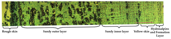
Figure 1.
Schematic composition of natural rubber bark.
2.1.1. Determination of the Density of Natural Rubber Bark
Density is defined as the mass of an object per unit volume. Density plays a crucial role in designing agricultural machinery and analyzing agricultural products. Various methods are employed for measuring density, such as the immersion method, gas displacement method, and density gradient tube method. To closely resemble the real-world conditions of rubber cutter shavings, we acquired natural rubber bark through standard rubber tree cutting procedures. Notably, the dry rubber on the sample’s surface was left incompletely cleaned. Given the strong water resistance of dried rubber, we determined the density of rubber bark in this section using the soaking method.
In the natural rubber forest, we randomly selected 10 natural rubber trees and obtained a specific mass of natural rubber bark, which was then transported to the laboratory. We removed only the dry rubber present as a mass on the bark’s surface (see Figure 2). The water content was measured at 63.7%, and the bark exhibited minimal water absorption, essentially negligible. Under room temperature conditions, the processed natural rubber bark is initially weighed using an electronic scale (I2000 type, accuracy of 0.1 g) (see Figure 3a) to determine its mass. Subsequently, it is submerged in a measuring cylinder filled with a specific volume of water, and the volume of the rubber bark is determined by observing changes in the water level (see Figure 3b). The density of natural rubber bark is calculated as follows:
where
—density of natural rubber bark (g·cm−3);
—mass of natural rubber bark (g);
—volume of water drained from the natural rubber bark (cm3).
We repeated the above measurement steps for a total of 10 groups and calculated the average value; the results obtained are shown in Table 1.

Table 1.
Measurements of natural rubber bark density.
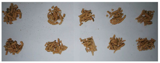
Figure 2.
Natural rubber bark test sample.
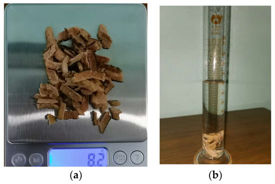
Figure 3.
Schematic diagram of natural rubber bark density measurement. (a) Mass measurement. (b) Volume measurement.
2.1.2. Determination of Poisson’s Ratio of Natural Rubber Bark
Poisson’s ratio, also known as the transverse deformation coefficient, represents the ratio of transverse positive strain to axial positive strain experienced by a material under unidirectional tension or compression.
Eight samples were taken from randomly selected rubber barks of a 10 mm × 10 mm × 10 mm specification size from natural rubber forests (Figure 4).
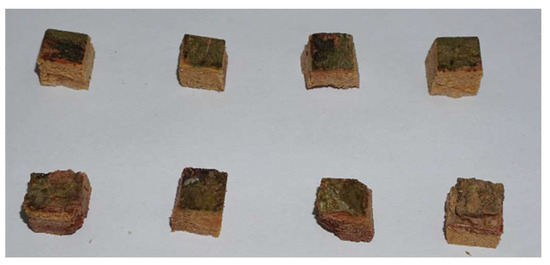
Figure 4.
Sample for determination of Poisson’s ratio of natural rubber bark.
We measured the width and length of natural rubber bark before compression using electronic digital calipers (accuracy: 0.1 mm). Subsequently, a compression test was conducted on the rubber bark employing an electronic universal testing machine (Instron 3369, 50 kN, accuracy: 0.00001 N) following the GB/T 1939–2009 Standard [27] for Compression Resistance Testing of Wood’s Cross Grain (see Figure 5). The loading speed was set to 5 mm/min (see Figure 4 and Figure 5).
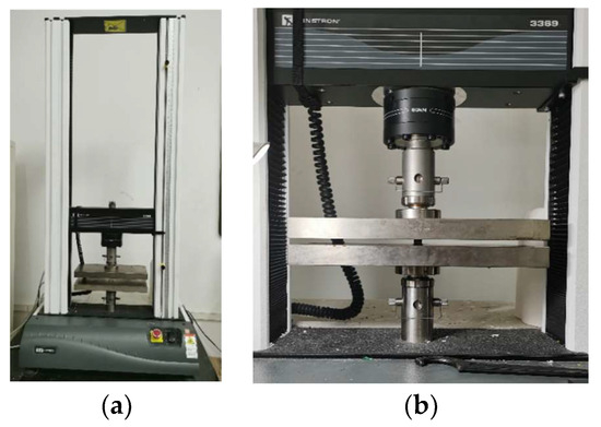
Figure 5.
Electronic universal testing machine and test process diagram. (a) Electronic universal testing machine. (b) Test procedure.
We measured the axial deformation of the compressed natural rubber bark using an electronic universal testing machine, and the lateral deformation was obtained using an electronic digital caliper. Subsequently, we calculated the Poisson’s ratio of the rubber bark as follows:
where
—Poisson’s ratio of natural rubber bark;
—Transverse deformation of natural rubber bark (mm);
—Axial deformation of natural rubber bark (mm);
—Transverse dimension of natural rubber bark before compression (mm);
—Transverse dimension of natural rubber bark after compression (mm);
—Axial dimension of natural rubber bark before compression (mm);
—Axial dimensions of natural rubber bark after compression (mm).
We repeated the above test steps 16 times, for a total of 16 groups of test results, and took the average value to find the natural rubber bark’s Poisson ratio = 0.379.
2.1.3. Determination of the Modulus of Elasticity of Natural Rubber Bark
The modulus of elasticity represents the direct relationship between stress and strain during the elastic deformation phase of a material, and its proportional coefficient is referred to as the modulus of elasticity. Measuring the modulus of elasticity of natural rubber bark provides insights into its resistance to elastic deformation.
Eight rubber bark samples were randomly collected from individual natural rubber trees and then trimmed to 10 mm × 10 mm × 10 mm dimensions, as illustrated in Figure 6. Electronic digital calipers were used for precise measurements of the thickness and width of the rubber bark before compression, enabling the determination of its cross-sectional area. Subsequently, each sample was positioned on the electronic universal testing machine’s test platform. A 50 mm diameter circular indenter applied load to the rubber bark, with a loading speed of 5 mm/min and a loading distance of 8 mm, as depicted in Figure 7. The resulting displacement-load data were recorded. The change in thickness of the rubber bark due to the applied load was determined by subtracting the displacement value at the maximum load point during the elastic deformation stage from the initial displacement value recorded in the displacement-load data. The modulus of elasticity of the natural rubber bark was calculated using the formula:
where
—modulus of elasticity of natural rubber bark (MPa);
—the maximum bearing force of the natural rubber bark at the stage of elastic deformation (N);
—initial thickness of natural rubber bark (mm);
—cross-sectional area of natural rubber bark (mm2);
—The difference in thickness of the natural rubber bark before and after the application of the load (mm).
The shear modulus of natural rubber bark can be obtained from the Poisson ratio and elastic modulus obtained from the above test, calculated as:
where —Natural rubber bark shear modulus (Mpa).
The above test steps were repeated 8 times and averaged and the results obtained are shown in Table 2.
Table 2.
Measurements of the modulus of elasticity of natural rubber bark.
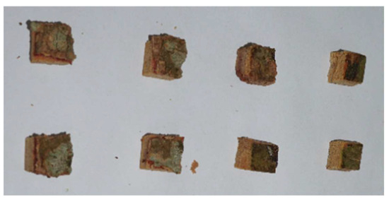
Figure 6.
Sample for the determination of the modulus of elasticity of natural rubber bark.
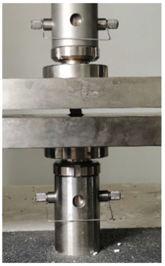
Figure 7.
Applied load process diagram.
2.1.4. Calibration of Crash Recovery Coefficient of Natural Rubber Bark
The collision recovery coefficient assesses a material’s capacity to restore its initial state after a collision, being solely tied to the material’s properties. It is defined as the ratio of the measured relative separation speed in the normal direction following a collision to the relative approach speed in the normal direction prior to the collision.
During testing, the small size of the natural rubber bark drop sample necessitates neglecting air resistance. The sample falls under the sole influence of gravity, and its relative approach velocity in the normal direction before colliding with the target material is determined by the kinetic energy theorem.
where
—Normal relative approach velocity before collision (m/s);
—Gravity acceleration (m/s2);
—Height of the rubber tree drop sample before the collision occurred (mm).
The normal relative separation velocity of the natural rubber tree bark drop sample after the collision with the collided material is
where
—Normal relative separation velocity after collision (m/s);
—Maximum rebound height of a falling sample of natural rubber bark after a collision (mm).
Based on the previous definition of the collision recovery coefficient, the formula for the collision recovery coefficient can be obtained as
Consequently, in the course of the test, measurements were limited to the drop height and the maximum rebound height of the natural rubber bark drop sample. The experimental setup is depicted in Figure 8. This paper primarily focuses on determining the impact recovery coefficients between natural rubber bark and 3Cr13 steel, as well as between natural rubber bark and other natural rubber bark samples.
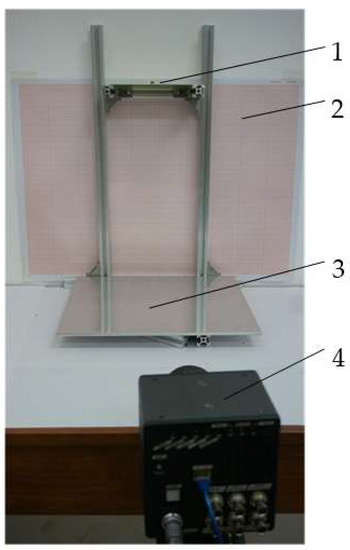
Figure 8.
Test stand: 1. Bark sample placement platform 2. Coordinate paper. 3. Collided material platform 4. High speed camera.
Natural rubber bark samples used in this test were derived from ten randomly selected normal-growth rubber trees in rubber forests. These samples were subsequently transported to the laboratory and further reduced to 5 mm × 5 mm × 5 mm dimensions for the drop test, as illustrated in Figure 9a. To ensure accurate shooting angles and prevent reading errors arising from incorrect camera angles during testing, the high-speed video camera’s lens was initially oriented horizontally on the collision material platform. Subsequently, the 3Cr13 steel plate was secured onto the collision material platform, as depicted in Figure 9b. Following this, the platform for dropping bark samples was set to a height of 350 mm. The rubber bark drop sample was released freely from this platform, horizontally colliding with the 3Cr13 steel plate and rebounding to a specific height. A high-speed video camera (Japan Photron Mini AX200 Ultra High Sensitivity High Speed Camera purchased from Chengdu Guangna Technology Co.) was employed to record the sample at a frame rate of 600 fps. The entire movement of the rubber bark drop sample was recorded using a high-speed camera (Photron Mini AX200) at a shooting speed of 600 fps, as depicted in Figure 10a. Concurrently, the photographs were imported into the computer in real-time to determine the maximum rebound height of the rubber bark drop sample following its collision with the 3Cr13 steel plate. For the collision recovery test involving rubber bark-to-rubber bark interactions, sheet rubber bark sourced from natural rubber forests was affixed to the collision material platform, as illustrated in Figure 9c. Subsequently, the remaining procedures were replicated as described earlier (Figure 10b). Ten separate data sets were tested and subsequently averaged. The tested results are presented in Table 3.
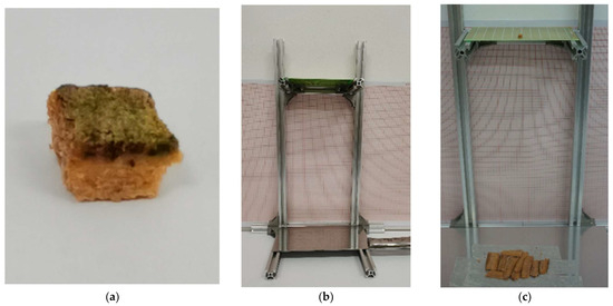
Figure 9.
Bark samples and drop test rigs. (a). Natural rubber bark sample. (b). 3Cr13 steel. (c). Rubber bark.
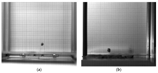
Figure 10.
High-speed camera recording test process diagram. (a). Rubber bark with 3Cr13 steel. (b). Rubber bark with rubber bark.
Table 3.
Determination of the collision recovery coefficient of natural rubber bark.
2.1.5. Calibration of the Coefficient of Friction of Natural Rubber Bark Skin
The coefficient of friction quantifies the ratio of friction between two material surfaces and the vertical force exerted on one of the surfaces. This ratio is influenced by the roughness of the material surfaces and is independent of the contact area between the two materials. Depending on the nature of motion, the coefficient of friction can be classified into static friction coefficient and dynamic friction coefficient.
Prior to measurement, ten healthy rubber trees from the natural rubber forest were chosen. We collected rubber bark using our team’s developed progressive rubber cutter, which intelligently profiles the natural rubber. This process involved removing dried rubber lumps from the surface of the bark samples, as depicted in Figure 11. Within this section, we determined the static and dynamic friction coefficients between rubber bark and 3Cr13 steel, as well as between natural rubber bark samples. These measurements were conducted using the ZOT-6027 friction coefficient tester with an accuracy of 0.001, as shown in Figure 12.
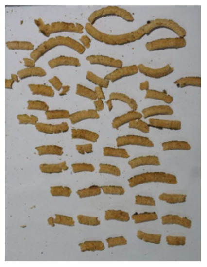
Figure 11.
Rubber Bark Sample.
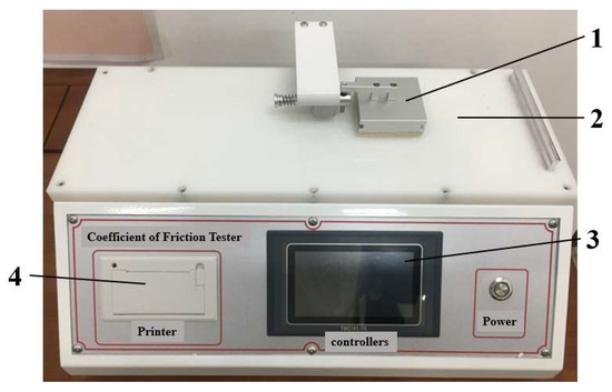
Figure 12.
Friction coefficient measuring instrument: 1. Slider 2. Horizontal test platform 3. Operation interface 4. Data printing outlet.
To measure the dynamic and static friction coefficients between natural rubber bark and 3Cr13 steel, we initially secured the 3Cr13 steel onto the horizontal test platform of the friction coefficient tester. Next, we placed the acquired rubber bark samples beneath the corresponding slider of the instrument. Subsequently, we conducted the friction coefficient test at a speed of 100 mm/min with a 60 mm moving distance, as illustrated in Figure 13a. After completing the test, we generated a printout of the test data. Following the completion of the test, we printed the test data. Each rubber bark sample underwent the test twice, resulting in a total of 20 sets of test data. We calculated the average values to determine the dynamic and static coefficients of friction between the rubber bark and 3Cr13 steel. In measuring the coefficients of static and dynamic friction between natural rubber bark samples, we affixed the natural rubber bark onto the horizontal test platform of the friction coefficient tester, as shown in Figure 13b. We then repeated the aforementioned steps to determine the coefficients of static and dynamic friction between natural rubber bark samples. The coefficient of friction values between rubber bark and 3Cr13 steel, as well as between natural rubber bark samples, are presented in Table 4.
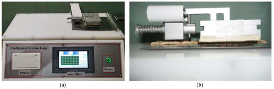
Figure 13.
Test process diagram. (a) Natural rubber bark with 3Cr13 steel. (b) Natural rubber bark and natural rubber bark.
Table 4.
Measurements of the coefficient of friction of natural rubber bark.
3. Results and Analysis
3.1. Discrete Elemental Modeling of Natural Rubber Bark
The discrete element model incorporates the Hertz–Mindlin with bonding model, enabling simulation of the material crushing and fracture resulting from small particle bonding. The sand bark cortex of natural rubber bark primarily consists of particles, and the presence of internal emulsion tubes imparts adhesive properties, akin to the natural rubber bark cut by a rubber knife. Thus, in this section, we employ the Hertz–Mindlin with bonding model to construct a discrete element model of natural rubber bark, and we define the corresponding bonding parameters based on literature [28], presented in Table 5.
Table 5.
Natural rubber bark Hertz–Mindlin with bonding model bonding parameters.
The bark of the natural rubber tree comprises distinct layers: rough bark, outer sandy bark, inner sandy bark, yellow bark, water bladder bark, and the formation layer. Rough bark constitutes approximately 8% of the total thickness, sandy bark comprises roughly 80%, and yellow bark constitutes around 7%. The combined thickness of the water bladder skin and the formation layer is merely 5%, making it almost negligible. To sustain continuous rubber production from the natural rubber tree, the layers of bark, starting from the rough to the yellow, must be selectively removed during tapping. While the physical structure of rubber bark is complex, and its components exhibit anisotropic behavior, accurately modeling its true properties presents a formidable challenge. In both domestic and international studies, anisotropy is often approximated as isotropy. Thus, due to current constraints in personnel, materials, and time, we have temporarily adopted an isotropic representation of rubber bark for this study. With the EDEM 2018 software, the rubber tree trunk was modeled as a standard cylinder with a reference circumference of C = 741 mm, resulting in a discrete element model of the rubber trunk with a diameter of 118 mm. For the purpose of simplifying calculations, enhancing the speed of discrete element model construction, and improving later simulation efficiency, we removed the inner cortex section of the rubber bark that does not participate in rubber cutting. Subsequently, we constructed a discrete element model of the rubber bark with a ring-like structure. Using research findings on the physical properties and contact characteristics of natural rubber bark (Table 6) as a basis, we utilized the particle factory plug-in to set the particle radius at 2 mm. Typically, the bonding radius of particles is 1.1–2 times their radius; we selected 2.5 mm for this parameter. With a dynamic particle generation rate of 5000 particles per second, we established a total of 120,000 particles in the discrete metamodel of natural rubber bark (Figure 14).
Table 6.
Table of simulation parameters for the discrete elemental model of natural rubber bark.
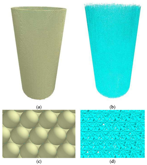
Figure 14.
Discrete elemental modeling of natural rubber bark. (a) Particle model diagrams. (b) Bonding bond model diagram. (c) Pellet detail. (d) Detailed view of bonding key.
3.2. Parameter Calibration and Model Validation
To ascertain the reliability and accuracy of the discrete element model for natural rubber bark, we conducted both simulation tests and real tests (Figure 15 and Figure 16) for shear and compression. This allowed us to compare the simulated test curves with their real counterparts, analyzing trends and relative stress errors. This comprehensive approach confirms the established model’s accuracy and reliability. This aims to validate the established model’s accuracy and reliability. Using the EDEM post-processing module, we derived and compared the shear force and compression force over time curves with the real test curves, as depicted in Figure 17.
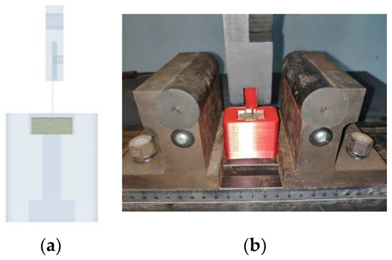
Figure 15.
Shear verification test. (a) Simulated shear test. (b) Real shear test.
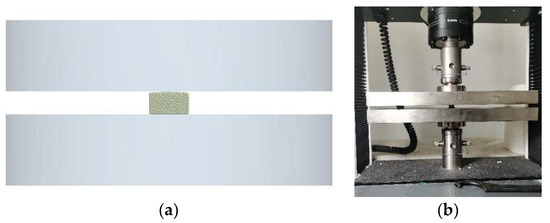
Figure 16.
Compression verification test. (a) Simulated compression test. (b) Real compression test.
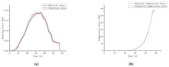
Figure 17.
Comparative test curves in shear and compression. (a) Shear test comparison curve. (b) Compression test comparison curve.
Figure 17a illustrates that both the simulation and real shear force with time exhibit an initial growth followed by a decrease. Specifically, from 0 to 150 s, the shear force demonstrates nearly linear growth. Between 150 and 200 s, fluctuations occur due to the rubber bark reaching its peak shear force, causing structural damage. During 200 to 285 s, the shear force displays a declining trend. This comparative analysis indicates significant similarity between the simulation and real shear tests in terms of the overall trend. The maximum shear forces recorded during shearing were 192.5 N and 188.6 N, with a relative error of only 2.1%.
Figure 17b reveals that both simulation and real compression forces initially increase, then decrease, briefly increase again, and eventually stabilize. The compression force remains nearly constant from 0 to 45 s. Between 45 and 85 s, both simulation and real compression forces increased, but the shear force decreased between 85 and 86 s. This decrease is primarily due to the rubber bark reaching its compressive limit, leading to structural damage and an abrupt drop in compression force, resulting in a brief downward trend in the curves. Between 86 and 94 s, both simulation and real compression forces continued to rise, while between 94 and 100 s, these forces remained relatively stable. This stability occurred because the rubber bark’s structure had been entirely compromised by this stage. The results indicate a striking similarity in the overall compression force trends over time between the simulated and real compression tests. The critical compression forces are 25.7 kN and 26.2 kN, respectively, with a mere 1.9% relative error between them. In summary, the simulation tests for shear and compression, along with the physical test results, exhibit a small relative error, confirming the reliability and accuracy of the established discrete element model for natural rubber bark. This model closely aligns with the mechanical and physical properties of real rubber bark, making it a suitable tool for characterizing actual rubber bark in relevant simulation tests.
4. Discussion
In field mechanized rubber cutting, the “L” cutter (Figure 18a) is commonly employed to cut along the pre-existing cutting line on the rubber tree. This line comprises solely two cutting surfaces: the lower surface and the inner side of the flow line. Yet, during the EDEM discrete element simulation test, modeling rubber bark that includes the open cutting line necessitates the creation of numerous discrete element particle models with varying trajectory inclinations. This process is both time-consuming and inefficient. Thus, the discrete element model created to represent the intact natural rubber bark, i.e., uncut, replicates the same two cutting surfaces found in field mechanized rubber cutting. Additionally, it incorporates a rubber flow line on the upper surface of the cutting area. Consequently, it becomes necessary to establish a “U-shaped” simulation of the rubber knife equipped with three blades.
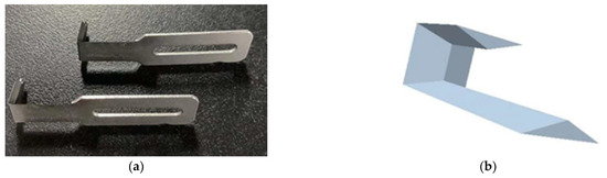
Figure 18.
Actual cutter and simulation test cutter models. (a) Actual cutter. (b) Simulation test cutter model.
We generated a 3D model of the cutter, matching the dimensions of the real cutter, using SolidWorks 2019 (Figure 18b). Subsequently, we imported this model into the EDEM2018 software in Parasolid format.
To determine the optimal cutting angle for the rubber cutter, aiming to minimize shear force, and to analyze its cutting performance at various angles, we conducted a one-factor discrete element simulation test on the rubber cutter. Referring to the “Rubber Tree Cutting Technical Regulations” by the Chinese Academy of Tropical Agricultural Sciences, we determined that cutting angles between 25° and 30° are optimal for male knife rubber cutting. In this study, we evaluated the shear force values of the rubber cutter at cutting angles ranging from 25° to 30° to determine the optimal cutting angle for rubber cutting.
The simulation test, illustrated in Figure 19, reveals the bond-breaking process among rubber bark particles. At 0 s (Figure 19a), the rubber cutting knife is positioned at the designated starting point, yet to initiate cutting of the natural rubber bark. Figure 19b–f depict the bond-breaking progression during the initial 5 s of rubber cutting. These figures demonstrate that, during the cutting process, the rubber cutter’s extrusion leads to the scattering fracture of particle bonding bonds in the forward direction of the cutter, centered around its blade. Consequently, we recorded shear force values at each time node and calculated their average over the simulation period. The results are presented in Table 7.
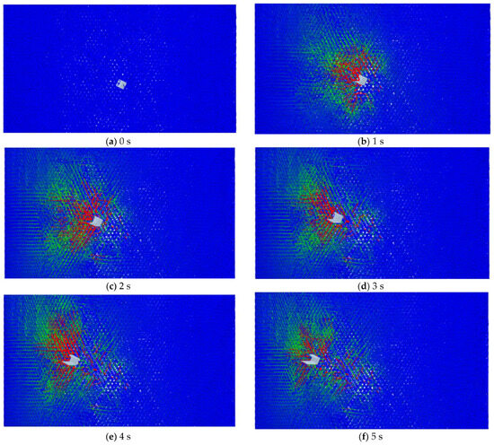
Figure 19.
Particle bond-breaking process.
Table 7.
Average shear force values for each cutting angle of the rubber cutter.
The results presented above underwent curve fitting via the quadratic Fourier fitting, as illustrated in Figure 20. This process was undertaken to derive the curve-fitted equations representing the average shear values corresponding to various cutting angles of the glue cutter.
where
= 117.7 with 95% confidence bounds (12.63, 222.7);
= −36.01 with 95% confidence bounds (−364.3, 292.3);
= −18.22 with 95% confidence bounds (−322, 285.6);
= 14.33 with 95% confidence bounds (−279.1, 307.7);
= 12.71 with 95% confidence bounds (−240.8, 266.2);
= 0.4774 with 95% confidence bounds (0.108, 0.8468).
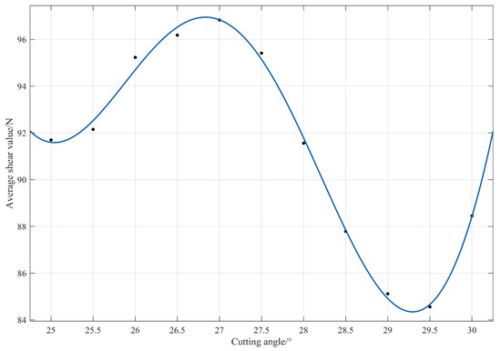
Figure 20.
Fitted curves of simulation analysis results.
The residual sum of squares is 0.7373, R2 is 0.9923, and the root mean square error is 0.384, which indicates a good fit for the model. Referring to Figure 20, we observe that the fitted Equation (8) exhibits a monotonically decreasing and then increasing pattern within the range of (27°, 30°). In this interval, the equation yields a very small value of 84.345 N, corresponding to a cutting angle of 29.294°. This analysis leads us to conclude that the optimal cutting angle for the rubber cutter is 29.294°. We assessed power consumption and the initial 5 min discharge volume as evaluation indices for measuring the power consumption of rubber cutting across various cutting angles of the rubber cutting knife. After conducting extensive statistical analyses based on field rubber-cutting tests in the forest (Figure 21), the results, presented in Table 8, demonstrate that when rubber cutting occurs at the optimal cutting angle, power consumption is 0.96 W-h, and the initial 5 min discharge volume is 6.53 mL. This optimization reduces the power consumption of the intelligent natural rubber cutting equipment by approximately 15% and extends the equipment’s usage time by about 20%.
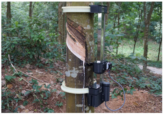
Figure 21.
Field cutting trials in natural rubber forests.
Table 8.
Average power consumption of 5 cuts with different cutting angles of the cutter and the amount of rubber discharged in the first 5 min.
5. Conclusions
- This paper is based on tests conducted in the natural rubber test forest area at Hainan University Danzhou. The natural rubber bark exhibited an average density of 1.23 g/cm3, a Poisson’s ratio of 0.379, an average modulus of elasticity of 18.09 MPa, and a shear modulus of 6.56 MPa. Additionally, the average collision recovery coefficient between natural rubber bark and 3Cr13 steel was 0.291, with dynamic and static friction coefficients of 0.515 and 0.651, respectively. The average collision recovery coefficient among natural rubber bark was 0.261, with dynamic and static friction coefficients of 0.841 and 1.338, respectively.
- We employed the discrete element method to create a model of natural rubber bark using the Hertz–Mindlin bonding contact model. After parameter calibration and model validation, we conducted a one-factor simulation test involving 11 different types of natural rubber bark, each with cutting angles ranging from 25° to 30°. We employed quadratic Fourier fitting to analyze the average shear force values obtained from the simulation for each cutting angle. The results revealed the minimum average shear force value of the rubber cutter in the [25°, 30°] range was 84.345 N, occurring at a cutting angle of 29.294°. This implies that rubber cutting at this angle offers low resistance, reducing power consumption.
- We employed the average power consumption and the initial 5 min rubber discharge volume as evaluation criteria for assessing rubber-cutting power consumption. After conducting numerous statistical analyses on field rubber-cutting tests in the forest, we found that the average power consumption for rubber cutting at a 29.294° angle was 0.96 W·h, with a rubber discharge volume of 6.53 mL within the first 5 min. These findings hold significant importance for optimizing natural rubber intelligent cutting equipment and its key components.
Author Contributions
H.Z.: conceptualization, methodology, investigation, and writing—original draft. Z.W.: investigation and writing—review and editing. Y.C.: writing—review and editing. J.L.: writing—review and editing. H.L.: writing—review and editing. Z.Z.: writing—review and editing. X.Z.: conceptualization, writing—review and editing, project administration and funding acquisition. All authors have read and agreed to the published version of the manuscript.
Funding
This work was supported by the Innovation Platform for Academicians of Hainan Province (Grant No. YSPTZX202109, YSPTZX202008), the Natural Science Foundation of Hainan Province (Grant No. 523RC440), the Key Research and Development Projects of Hainan Province (Grant No. ZDYF2021XDNY198), Science and Technology Innovation Project of Sanya (Grant No. 2022KJCX94), the National Modern Agricultural Industry Technology System Project (Grant No. CARS-33-JX2), the Scientific Research Project of Hainan Province (Grant No. Hnky2022-9), the Research Start-up Funding Projects of Hainan university (Grant No. KYQD(ZR)-22036), the Hundreds and Thousands Science and Technology Major Project of Heilongjiang Province (Grant No. 2020ZX17B01-2).
Institutional Review Board Statement
Not applicable.
Informed Consent Statement
Not applicable.
Data Availability Statement
Not applicable.
Conflicts of Interest
The authors declare that there are no conflict of interest.
References
- Sivaselvi, K.; Gopal, K. Study to enhance the mechanical properties of natural rubber by using the carbon black (N550). Mater. Today Proc. 2020, 26, 378–381. [Google Scholar] [CrossRef]
- Zheng, T.; Zheng, X.; Zhan, S.; Zhou, J.; Liao, S. Study on the ozone aging mechanism of Natural Rubber. Polym. Degrad. Stabil. 2021, 186, 109514. [Google Scholar] [CrossRef]
- Guo, Y.; Bao, K.; Wu, X.; Han, D.; Zhang, J. Morphology and aggregation process of natural rubber particles. Ind. Crop Prod. 2023, 203, 117153. [Google Scholar] [CrossRef]
- Stoček, R.; Heinrich, G.; Kipscholl, R.; Kratina, O. Cut & chip wear of rubbers in a range from low up to high severity conditions. Appl. Surf. Sci. Adv. 2021, 6, 100152. [Google Scholar]
- Zhang, H.; Chen, Y.; Cong, J.; Liu, J.; Zhang, Z.; Zhang, X. Reliability Study of an Intelligent Profiling Progressive Automatic Glue Cutter Based on the Improved FMECA Method. Agriculture 2023, 13, 1475. [Google Scholar] [CrossRef]
- Zhao, H.; Huang, Y.; Liu, Z.; Liu, W.; Zheng, Z. Applications of Discrete Element Method in the Research of Agricultural Machinery: A Review. Agriculture 2021, 11, 425. [Google Scholar] [CrossRef]
- Horabik, J.; Molenda, M. Parameters and contact models for DEM simulations of agricultural granular materials: A review. Biosyst. Eng. 2016, 147, 206–225. [Google Scholar] [CrossRef]
- Cong, J.; Wang, X.; Yan, C.; Yang, L.T.; Dong, M.; Ota, K. CRB Weighted Source Localization Method Based on Deep Neural Networks in Multi-UAV Network. IEEE Internet Things 2023, 10, 5747–5759. [Google Scholar] [CrossRef]
- Cong, J.; Wang, X.; Lan, X.; Liu, W. A Generalized Noise Reconstruction Approach for Robust DOA Estimation. IEEE Trans. Radar Syst. 2023, 1, 382–394. [Google Scholar] [CrossRef]
- Ucgul, M.; Saunders, C. Simulation of tillage forces and furrow profile during soil-mouldboard plough interaction using discrete element modelling. Biosyst. Eng. 2020, 190, 58–70. [Google Scholar]
- Shi, G.; Li, J.; Ding, L.; Zhang, Z.; Ding, H.; Li, N.; Kan, Z. Calibration and Tests for the Discrete Element Simulation Parameters of Fallen Jujube Fruit. Agriculture 2022, 12, 38. [Google Scholar] [CrossRef]
- Dai, Z.; Wu, M.; Fang, Z.; Qu, Y. Calibration and Verification Test of Lily Bulb Simulation Parameters Based on Discrete Element Method. Appl. Sci. 2021, 11, 10749. [Google Scholar] [CrossRef]
- Horabik, J.; Wiącek, J.; Parafiniuk, P.; Bańda, M.; Kobyłka, R.; Stasiak, M.; Molenda, M. Calibration of discrete-element-method model parameters of bulk wheat for storage. Biosyst. Eng. 2020, 200, 298–314. [Google Scholar] [CrossRef]
- Dai, L.; Sorkin, V.; Vastola, G.; Zhang, Y.W. Dynamics calibration of particle sandpile packing characteristics via discrete element method. Powder Technol. 2019, 347, 220–226. [Google Scholar] [CrossRef]
- Fang, M.; Yu, Z.; Zhang, W.; Cao, J.; Liu, W. Friction coefficient calibration of corn stalk particle mixtures using Plackett-Burman design and response surface methodology. Powder Technol. 2022, 396, 731–742. [Google Scholar] [CrossRef]
- Liu, R.; Liu, L.; Li, Y.; Liu, Z.; Zhao, J.; Liu, Y.; Zhang, X. Numerical Simulation of Seed-Movement Characteristics in New Maize Delivery Device. Agriculture 2022, 12, 1944. [Google Scholar] [CrossRef]
- Wang, M.; Liu, Q.; Ou, Y.; Zou, X. Numerical Simulation and Verification of Seed-Filling Performance of Single-Bud Billet Sugarcane Seed-Metering Device Based on EDEM. Agriculture 2022, 12, 983. [Google Scholar] [CrossRef]
- Chen, Z.; Wassgren, C.; Ambrose, R.P.K. Development and validation of a DEM model for predicting impact damage of maize kernels. Biosyst. Eng. 2022, 224, 16–33. [Google Scholar] [CrossRef]
- Kim, Y.; Lee, S.; Baek, S.; Baek, S.; Jeon, H.; Lee, J.; Abu Ayub Siddique, M.; Kim, Y.; Kim, W.; Sim, T.; et al. Development of DEM-MBD coupling model for draft force prediction of agricultural tractor with plowing depth. Comput. Electron. Agr. 2022, 202, 107405. [Google Scholar] [CrossRef]
- ASAE D497.4; Agricultural Machinery Management Data. American Society of Agricultural and Biological Engineers ASABE: St. Joseph, MI, USA, 2000.
- Foldager, F.F.; Munkholm, L.J.; Balling, O.; Serban, R.; Negrut, D.; Heck, R.J.; Green, O. Modeling soil aggregate fracture using the discrete element method. Soil. Tillage Res. 2022, 218, 105295. [Google Scholar] [CrossRef]
- Azimi-Nejadian, H.; Karparvarfard, S.H.; Naderi-Boldaji, M. Weed seed burial as affected by mouldboard design parameters, ploughing depth and speed: DEM simulations and experimental validation. Biosyst. Eng. 2022, 216, 79–92. [Google Scholar] [CrossRef]
- Huang, T.; Cao, L.; Zhang, X.; Ding, H. Necessary discrete condition for error control of time-domain methods in milling stability prediction. Nonlinear Dynam. 2021, 104, 3771–3780. [Google Scholar] [CrossRef]
- Yoon, H.S.; Ehmann, K.F. Dynamics and stability of micro-cutting operations. Int. J. Mech. Sci. 2016, 115-116, 81–92. [Google Scholar] [CrossRef]
- Azvar, M.; Budak, E. Multi-dimensional chatter stability for enhanced productivity in different parallel turning strategies. Int. J. Mach. Tools Manuf. 2017, 123, 116–128. [Google Scholar] [CrossRef]
- Yan, Y.; Xu, J.; Wiercigroch, M. Estimation and improvement of cutting safety. Nonlinear Dynam. 2019, 98, 2975–2988. [Google Scholar] [CrossRef]
- GB/T 1939-2009; Test Method for Transverse Grain Compression of Wood. Standardization Administration of China: Beijing, China, 2009.
- Cao, C.; Zhang, X.; Fu, W.; Xing, J.; Liu, J.; Zeng, W. Calibration and verification of the parameters of the discrete element simulation model of natural rubber tree skin characteristics. J. Shihezi Univ. (Nat. Sci.) 2022, 40, 691–697. [Google Scholar]
Disclaimer/Publisher’s Note: The statements, opinions and data contained in all publications are solely those of the individual author(s) and contributor(s) and not of MDPI and/or the editor(s). MDPI and/or the editor(s) disclaim responsibility for any injury to people or property resulting from any ideas, methods, instructions or products referred to in the content. |
© 2023 by the authors. Licensee MDPI, Basel, Switzerland. This article is an open access article distributed under the terms and conditions of the Creative Commons Attribution (CC BY) license (https://creativecommons.org/licenses/by/4.0/).