Abstract
The detection of possible areas for the application of agroforestry is essential and involves the usage of various technics. The recognition of forest types using satellite or aerial imagery is the first step toward this goal. This is a tedious task involving the application of remote sensing techniques and a variety of computer software. The overall performance of this approach is very good and the resulting land use maps can be considered of high accuracy. However, there is also the need for performing high-speed characterization using techniques that can determine forest types automatically and produce quick and acceptable results without the need for specific software. This paper presents a comprehensive methodology that uses Normalized Difference Vegetation Index (NDVI) data derived from the Moderate Resolution Imaging Spectroradiometer instrument (MODIS) aboard the TERRA satellite. The software developed automatically downloads data using Google Earth Engine and processes them using Google Colab, which are both free-access platforms. The results from the analysis were exported to ArcGIS for evaluation and comparison against the CORINE land cover inventory using the latest update (2018).
1. Introduction
The land use management system in which trees or shrubs are grown around crops or pastures is called agroforestry. This combination of agricultural and forestry usages has multiple advantages: the improvement of erosion protection, an increase in biodiversity, carbon sequestration, etc. [1]. Mixed forest stands can be used for the establishment of agroforestry systems; therefore, forest type identification is an essential procedure for the application of environmental management practices as well as the identification of the proper agroforestry system that can be applied [1,2]. Forest types depend mainly on the geographical location of the forest, which, combined with different precipitation and evapotranspiration levels, is responsible for different biomes. Tropical moist and dry forests are located across the Equator, boreal forests are located around the North Pole and temperate forests are located at middle longitudes. Forests established on higher elevations tend to be more similar to forests located at higher latitudes [3]. In Europe and particularly in Greece, which is located between 41.50306 S and 35.01186 N, well inside the temperate zone, forests include broadleaf deciduous forests, evergreen coniferous forests and mixtures between these types [4].
Forests are considered the largest land carbon pools accounting approximately for 85% of the total land biomass [2]. The soil carbon stock of forests represents 73% of the total (global) soil carbon [5]. Based on this fact, forests are a key factor in ecosystem management for climate change mitigation and environmental improvement [6,7,8]. Mitigation can be applied by reducing forest degradation and increasing forest resources, which can be measured by performing an accurate mapping of forest types [9]. The typical method of forest surveying for the estimation of biomass includes random sampling and a field investigation of the selected plots, which is tedious and time-consuming work [10,11]. In order to speed up the process, remote sensing data can be used to obtain data from rural areas, locations on extreme slopes and difficult-to-reach locations. Data of this type can be combined with traditional methods to speed up forest surveying and reduce fieldwork. Remote sensing data can be obtained either from aerial imagery or through various satellite services [12]. Satellite data are very common these days especially due to the fact that many companies exist that provide them either free of charge (Glovis, United States Geological Survey (USGS) Earth Explorer, Copernicus, etc.) or at a cost (Landsat, Spot, Aster) depending on the region required as well as the extent of the timeframe [13]. It is up to the researcher to choose the type of data required for his research; however, it is common knowledge that free-of-charge services provided lower resolution data at limited timeframes whereas paid services provide several types of datasets at different resolutions and more timeframes [13].
Nevertheless, even the combination of the aforementioned methods can also prove to be insufficient, especially in the case where large areas must be mapped. This is mostly the case when research is required to determine the optimal agroforestry system to be applied in a certain area [14,15,16]. This paper describes a methodology for automating the entire procedure by proposing (and testing) an algorithm that automatically downloads data from the MODIS instrument of the TERRA satellite [17] using the Google Earth Engine and subsequently processes the data using Google Colab by applying a harmonic NDVI time series clustering to determine two main forest types (coniferous and mixed forests/broadleaved forests). The results are then compared to land use data from the CORINE land cover inventory. The methodology provided promising results, which can be further improved by applying machine learning methods such as artificial neural networks, random forests and expert systems [12,18,19], and the results can be used for the application of forest policy as well as decision making [20,21,22,23,24].
This paper is organized as follows. The introduction (Section 1) provides useful information regarding forest surveying and forest types, followed by the literature review where surveying methodologies are presented. Materials and methods (Section 2) describes the location used for the application of the methodology; the algorithm used; and the data used. Results (Section 3) presents in detail the results produced, including comparison maps and the clustering results. Section 4 is dedicated to a general discussion of the produced results and Section 5 for the conclusion where future improvements to the methodology are suggested. The presented methodology is an effort to automate the work presented by Jakubauskas [25,26] and test its application against forest land cover types.
Literature Review
NDVI is a simple index, which is often used to analyze remote sensing data and determine whether an area under study contains vegetation or not. NDVI is based on the usage of visible and near-visible (infrared—IR) parts of the electromagnetic spectrum to determine the existence of vegetation (as well as its health). This is performed by measuring the ratio between near-infrared (NIR) radiation (which is strongly reflected from vegetation) minus red (which is absorbed by vegetation) and NIR plus red. NDVI values range between −1 and +1. Low NDVI values indicate moisture-stressed vegetation and higher values indicate a higher density of green vegetation [27].
NDVI in combination with land cover type changes was used for the exploration of relationships between the NDVI values of different land cover types, air temperature and precipitation during the 1982–2015 period based on a dynamic grid. The results from this comparison indicated that forests and shrubland areas increased as a large area of grassland transformed to forest. Additionally, snow/ice tundra and grassland decreased during the same period [28]. A methodology for the estimation of the conifer–broadleaf ratio in mixed forests based on time series data was used by researchers at the Purple Mountain of the Jiangsu Province in China. The researchers tried to demonstrate the feasibility of accurately estimating the conifer–broadleaf ratio using satellite data and field measurements. In detail, leaf area index time series data and forest plot inventory data were acquired. The data were then imported to the invertible forest reflectance model (INFORM) for simulating the NDVI index of different conifer–broadleaf ratios. Fifteen Gaofen-1 (GF-1) satellite images of 2015 were acquired. The conifer–broadleaf ratio estimation was based on the GF-1 NDVI time series and semi-supervised K-means cluster method, which resulted a high overall accuracy of 83.75% [29].
Other researchers explored and evaluated the potential of freely available satellite imagery and an object-based random forest algorithm as a source for the identification of forest types. In detail they used datasets from Sentinel-2A, Sentinel 1A in dual polarization, a digital elevation model (DEM) from one-arc-second Space Shuttle Radar and LandSat 8 images. The usage of only satellite imagery had the least satisfactory results. The combination of satellite imagery with DEM data improved the identification result accuracy and the highest accuracy (82.78%) was achieved when using a combination of all data [30]. Forest composition mapping in various image availability conditions and how missing data due to clouds or scan line problems affect classification accuracy were explored by researchers [31]. In this research, a long-period (1 January 2014 to 31 December 2016) Landsat imagery dataset was used in an area where most forest stands were mixed. For classifying the type of stands, the researchers used decision trees and rule-based models implemented in R. The results were then compared to the Reconnaissance Forest Inventory Data (RECON) and showed that for pure stands the identification results were high ranging from 96.2% for northern hardwoods to less than 10% correct identification for tamarack. Eight-day composite MODIS NDVI data were used for the period between 2001 and 2014 to access the significant negative trend of seasonal natural vegetation in India. Forest phenology data were extracted from the MODIS NDVI series. Data were harmonized and a non-parametric trend analysis was applied (Mann–Kendall statistics and Theil–Sen slope). Four types of negative trends were produced [32]. Twenty-year-long MODIS NDVI data were also used for the estimation of spring vegetation green-up dynamics. In this study, data for a period staring on 2000 and ending to 2019 were used for calculating green-up duration (GUD). The GUD was calculated for 170,000 pixels for the wider Carpathian Basin and exhibited large interannual and elevation-dependent variability, which indicates the distribution of different species. The longest mean GUD occurred in 2017 (32.7 days) while the shortest (14.5 days) occurred in 2018 [33].
Finally, MODIS data were also used for the evolution assessment of the vegetation state and its relationship with the climate dynamics in the Mediterranean forest region of Tunisia using land surface phenology (LSP) and NDVI data from MODIS. The results showed that the LSP index changed significantly during the study period. Precipitation and maximum temperatures represent the best climate parameters to explain the changes in LSP. Finally, both NDVI and SPEI (standard precipitation-evapotranspiration index) indexes showed a significant correlation on longer time scales [34]. Evidently, satellite data in combination with the NDV index can be used for determining forest type, stand type, vegetation status, etc. [35]. However, data processing can be difficult and in many cases the data size required to be processed exceeds the capabilities of the average workstation [36].
All the aforementioned methods are trying to identify crop types or forest types using a combination of satellite data and machine learning algorithms. Additionally, all of them are optimized for producing optimal results in the case study area and/or specific fauna types. Therefore, it would be difficult to use in other zones. Furthermore, all these approaches share a common point, the exploitation of the NDV index. Result improvements for these methods can be achieved by using additional data for the study areas. These data can include the geographical location of the area (coordinates), the elevation derived from the digital elevation model of the area (if available), prior phytosociological data, etc. The usage of these data must be conducted carefully and in combination with the advice of an expert (forester, agronomist, etc.). A lot of errors can be produced if we try to generalize and match certain species with certain altitudes or geographic locations. For example, there is a general approach that combines evergreen conifers forests with northern latitudes and higher altitudes. Although correct, one cannot underestimate the fact that in southern countries (Greece, Spain, Italy, etc.) there are vast conifer forests located at sea level. Similarly, many broadleaved deciduous trees can exist at higher altitudes (Fagus sp., Ulmus sp., etc.). Therefore, the application zone plays a critical role on the results as well as their interpretation.
Obviously, it is up to the researcher to implement the optimal approach and additionally interpret the results produced by the application of the selected methodology. Finally, it must be noted that most of these methods must be modified substantially to be applied in other research areas and therefore cannot be easily generalized.
In the present study, we try to overcome the aforementioned restrictions and explore the possibility that the required satellite data are downloaded using a web service (Google Earth Engine—GEE) directly to a cloud programming platform (Google Colab—GC), are processed in order to calculate the harmonized NDV Index and clustered using the time series K-means clustering algorithm. The usage of a cloud programming platform such as GC has many advantages with the main one being that the user takes advantage of the massive computer infrastructure of Google to perform all the difficult and processor-intensive tasks. This approach allows the algorithm users to apply the methodology without the need to allocate local computer resources and additionally provides them with the capability to easily change the time period used for the satellite data.
Additionally, with Colab, users can create and share notebooks or documents, which can be simultaneously edited from Google Docs, supporting platforms and development collaborations regardless of the operating system each user has equipped or its location. Colab supports version 2.7 and 3 of the Python scripting language and can be easily accessed through Google’s browser Chrome. Finally, the software is also integrated with Google Drive, so users can easily share projects or copy others’ shared projects onto their own accounts. There is no need for high-end workstations to perform the work as it is performed on the Cloud.
2. Materials and Methods
2.1. Study Area
The proposed methodology was applied in the Drama prefecture, which is in Northern Greece, in Macedonia (Figure 1, left). The region is a part of the Rhodope Mountain Range, it is mostly covered by forest ecosystems, and it constitutes the oldest land mass of the Balkan Peninsula. The area is characterized by a diverse landscape, which includes grass meadows, pastures and wooden lands and it is grazed not only by domestic animals (cattle, sheep, etc.) but also by wild horses and red deer. The main forest species found are the following: Abies alba, Abies borissi regis, Picea alba, Pinus nigra, Pinus peuce, Fagus sylvatica, Carpinus orientalis and Quercus spp., which form various types of stands (conifer, broadleaf and mixed stands) [37]. The topography is characterized by steep slopes and mountains with many peaks above 2000 m, and the climate is characterized as Mediterranean (Csb according to Köppen climate classification) [38].
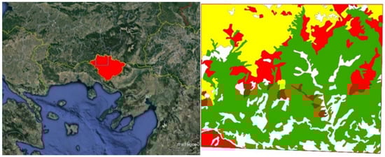
Figure 1.
Drama prefecture (left) in red and the polygon where the methodology was applied in light blue (image from Google Earth). Main forest land use types (right) from CORINE.
For this research, a polygon was randomly created by setting four random points, near the border with Bulgaria, covering an area of 82,568.36 ha. Additionally, CORINE 2018 land cover files were downloaded from the Copernicus Land Monitoring Service and processed using ESRI ArcMap, in order to include only the required land uses (broadleaved forests CLC 311, coniferous forests CLC 312, mixed forests CLC 313) for our study (CLC stands for Corine land cover and is a term used to characterize each polygon in the Corine Database). The total area covered by CLC 311, CLC 312 and CLC 313 land uses inside the study area is 69,954.82 Ha, or 84.72% of the total area (Figure 1, right).
2.2. Data Manipulation
The removal of the non-essential land uses was performed in two steps. At first, a structured query language (SQL) was applied on the CLC database to select only the required CLC area codes and their locations. The results from the query were exported to a database and a new, spatial query was performed to clip features that were outside the study area. Before the application of the methodology, we must perform some initial tasks, which are presented inside the dashed box on Figure 2, Environment Initialization. This initialization comprises all the essential steps that are needed to access Google Colab, the application programmable interface (API) and the installation of the required Python packages. Finally, during this process the user determines the coordinates (or sets them randomly) of the polygon vertexes where the methodology will be applied. This section is required to be performed only once at the beginning.
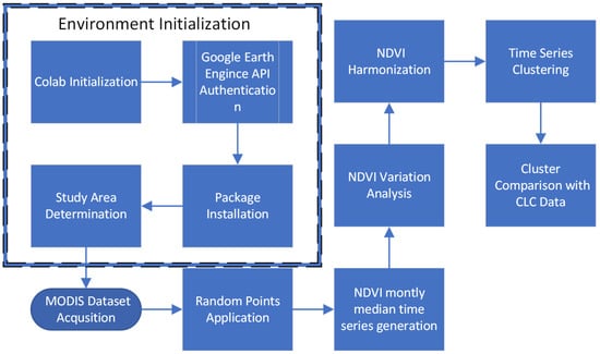
Figure 2.
Overall workflow, environment initialization (dashed box) and methodology.
The second section (Figure 2, outside of the dashed box) includes all the necessary steps to apply the methodology. These steps can be considered procedures and functions inside the algorithm. In detail, the steps are the following:
- MODIS dataset acquisition. In this step, the algorithm downloads all the required data for the study area and the time period specified by the user. The data include daily NDVI images from the MODIS satellite. The normalized difference vegetation index is generated from the near IR (NIR) and red (RED) bands as a ratio of (NIR − RED)/(NIR + RED) and the ratio values range between −1.0 and 1.0. The data are generated from the MODIS/006/MOD09GA surface reflectance composites. It is worth noting that all data are stored temporally on the cloud (Google Colab) and not locally on the user’s computer.
- Afterwards, we insert 100 randomly generated points and for these we estimate the median monthly NDVI values for each point (steps 2 and 3).
- The next step includes the usage of the ipygee tools for generating and viewing a chart of the NDVI variation on each point for the time period we defined (step 4).
- After the creation of the NDVI median chart, we apply the harmonic model (step 5). A Fourier (harmonic) analysis permits a complex curve (such as the one created in the previous step) to be expressed as a series of cosine waves (which are called terms) and an additive term [39].
- On the created harmonic model, we apply a clustering algorithm for the identification of samples with similar characteristics and therefore of the same origin and create the appropriate clusters. There are various clustering algorithms available, and in our case we used the time series K-means algorithm to cluster the samples.
2.3. Harmonic Analysis
In the harmonic (Fourier) analysis, each wave is defined by a unique amplitude and a phase angle, where the amplitude value is half the height of a wave, and the phase angle (or simply, phase) defines the offset between the origin and the peak of the wave over the range 0 to 2π (Figure 3A). Each term designates the number of complete cycles completed by a wave over the defined interval (Figure 3B). Successive harmonic terms are added to produce a complex curve (Figure 3C) and each component curve accounts for a percentage of the total variance in the original time series [39].
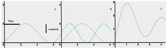
Figure 3.
(A) simple cosine curve, (B) curves for harmonic terms, (C) curve produced from addition of curves in (B).
The harmonic analysis of the time series we have created aims at determining possible seasonal changes in the spectral behavior of the points by performing a decomposition of the time series in harmonic terms. Most of the observed variance in the dataset is expected to be contained in the first period, similarly to other analysis such as the principal component analysis. Over 90% of the variance in the original time series was captured in the additive and the first two terms [25].
Harmonic analysis has been used for image and sound analysis [40,41,42,43] and for analyzing datasets of successive regular multidate samples of satellite imagery [44,45,46,47]. Especially in the case of land use and land use changes, harmonic analysis has been used to determine land use change on agricultural land in a yearlong period [25,26] and has proven as useful in that seasonal and interannual cycles (such as the ones produced by leaf drop in broadleaved forests) can be determined and highlighted.
2.4. Time Series Clustering
Time series data are considered one of the major data types, which are generated in huge quantities nowadays. Satellite data in particular (which are time stamped) create large data series of spatial measurements. In general, time series data are considered as supervised data but, when their generation becomes vast and fluctuate, they behave as unsupervised data (in general, supervised data use labeled input and output data, while unsupervised data do not). Thus, time series clustering is a process that can help us to cluster vast fluctuating time series data.
The main difference between time series data clustering and data clustering in general is that the data used contain time values, and we want to exploit this characteristic in order to identify possible time clusters. There are various methods for performing this type of clustering (agglomerative clustering, time series K-means, kernel K-means, etc.) [48]. In this paper, we use K-means time series clustering mainly because we try to group similar data points (median monthly NDVI values) and discover if there is an underlying pattern between NDVI values and different forest types. Additionally, K-means requires a fixed number of clusters (K), which is compatible with the approach we used, randomly placing 100 points. For the application of K-means, we defined k as 2 to determine the two main forest types (coniferous and mixed forests/broadleaved forests).
In the standard K-means algorithm, total within cluster variation is defined as the sum of the squared Euclidean distances between items and the corresponding centroid, which is shown in the following equation [49].
where xi is ith data point of cluster k (Ck), and μk is the mean value of points in cluster k. A quick algorithm for estimating the value of W is the following:
Data: k numbers of clusters;
Result: set of k cluster initialization.
While the centroids do no change, do the following:
- -
- Assign each point to its closest centroid;
- -
- Compute the new centroid (mean) of each cluster;
end while
In classic K-means clustering, we would consider the median monthly NDVI values on each location as data points, but by averaging data, valuable information would be lost. The usage of time series clustering helps us to overcome the issue by considering all data points simultaneously and grouping locations with similar time series into the same cluster.
3. Results
After the initialization of the platform, we set the boundaries of the study area, by determining its vertex’s coordinates. For this polygon we downloaded the NDVI data from MODIS/006/MOD09GA for the time period beginning on 1 January 2019 and ending on 31 December 2021. A three-year period was selected because we wanted to include land cover variance, which is generated both from season change and from change in meteorological conditions, which can also affect the NDV index of trees.
Afterwards, we inserted 100 randomly created points in order to apply the K-means time series clustering method. In Figure 4, we present the study areas’ polygon vertexes marked with red balloon icons. Inside the polygon depicted as red stars are the randomly created points (steps 2 and 3).
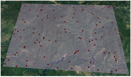
Figure 4.
Study area boundaries and random points.
Additionally, for each point we applied the ipygee tool to generate and view a chart of the NDVI variation on each point for the selected time period (Figure 5). The variation was graphically depicted using three colors (red, yellow, green) and it was also plotted as a chart, where the mean NDVI values were set on the y axis, and the associated time stamp on the x axis (Figure 5). It is evident that most of the value fluctuation is monitored on the first two harmonic terms (time periods).
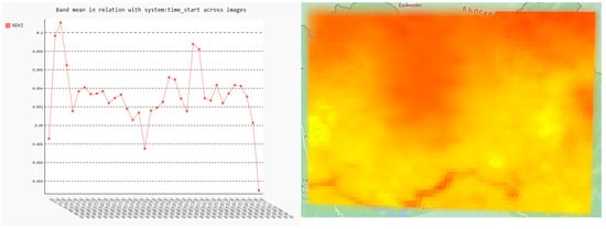
Figure 5.
Median monthly NDVI values.
For the calculated median monthly NDVI values we applied the harmonic model to decompose the time series presented in Figure 5 into harmonic terms. The additive term and the phase and amplitude for the first two harmonic terms were extracted and used for further analysis. The calculated harmonic terms for the MODIS NDVI time series as well as the graphical representation of these values are presented in Figure 6.
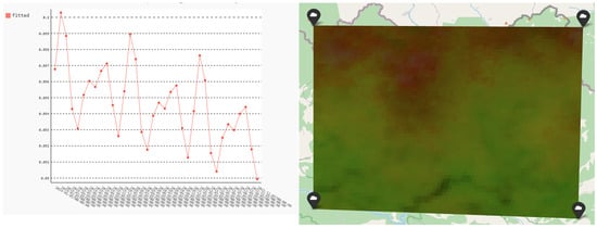
Figure 6.
Harmonized mean NDVI values.
Finally, for the harmonized mean NDVI values we applied the K-means time series clustering to cluster the harmonized mean NDVI values. The results are depicted on Figure 7.
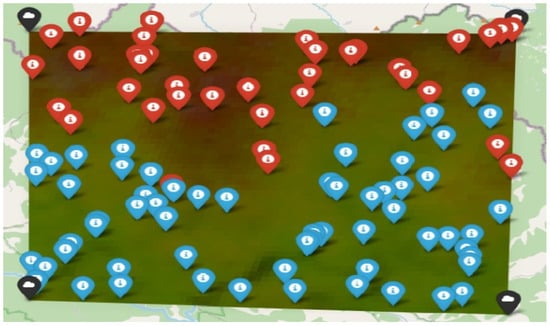
Figure 7.
Results from the application of time series clustering algorithm.
From Figure 7, it is evident that the algorithm has determined the existence of two classes. Broadleaved and mixed forests were estimated as one class and conifers as the other. In order to test the provided results, we must compare them with actual land use types. For this reason, we extracted the points and created a new geodatabase which was then compared with the CORINE 2018 land use data (Figure 8).
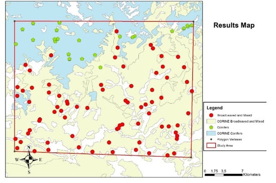
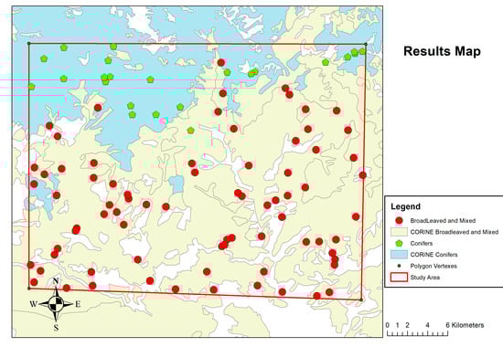
Figure 8.
Results comparison with CORINE 2018 CLC.
Obviously, from the results it is clear that the suggested methodology successfully managed to identify two major forest type stands. Conifer and broadleaved-mixed forest stands. In Table 1, we present the results from the methodology application regarding the correctly and incorrectly identified forest types.

Table 1.
Results.
4. Discussion
The results from the application of the methodology are encouraging. Out of the 100 randomly placed points, the amount of correctly identified conifers stands was 69.4% whereas the amount of correctly identified broadleaved-mixed stands was 87.5%.
The algorithm works better in the case of broadleaved and mixed forest stands. The difference in the results can be easily interpreted by the fact that the broadleaved-mixed forest stands present a strong seasonality in their appearance mainly due to the fact that they drop their leaves during the winter. We believe that this fact plays an important role in the accuracy of the proposed methodology as the NDVI variation is larger in these stands during winter. Similar results were also produced in other efforts to automate the identification of different land uses (crop types) where the correctly identified crop types ranged from 66% for wheat (Triticum aestivum) to 16% for milo (Sorghum bicolor) [25]; the identification of forest vegetation types using spatio-temporal fusion had an accuracy Kappa coefficient of 95.6% [50]; mapping crop types had an overall map accuracy of 75.5% [51]; and land cover with Google Earth Engine, optical images and supervised algorithms had results that showed 0.99% accuracy for the support vector machine, 0.95% for the random forest and 0.92% for classification and regression trees. The kappa index was as follows: 0.99% for the support vector machine, 0.97% for the random forest and 0.94% for classification and regression trees [52].
The algorithm could not successfully identify mixed stands from broadleaf stands, mainly due to the lack of proper resolution on the satellite data. In many cases, methodologies such as the one described are confounded by the spatial resolution of the images being produced by the scanner. Stands that are smaller than the resolution of the sensor cannot be identified correctly. The same goes in the case of mixed forest stands where in some cases the in-stand variations of the tree types (conifers and broadleaved) are small and therefore difficult to identify due to data resolution [53,54]. The MODIS/006/MOD09GA spatial resolution is 500 m; therefore, patches smaller than the spatial resolution cannot be identified correctly.
A significant improvement on the result accuracy could be achieved using high-resolution satellite imagery. Similarly, improvement can also be achieved by using a combination of satellite sources, which can result in overall better raw data.
Harmonic analysis can also be used as a tool for monitoring vegetation change [32]. Given that different land uses create different phase and amplitude values in the harmonic analysis, the produced results suggest that the methodology can also be used to detect changes in land use by examining changes in annual values of phase or amplitude. For example, changes in seasonal amplitude while the phase remains unchanged could indicate changes in vegetation condition. Changes in phases where the amplitude remains unchanged could indicate a change in the time of maximum greenness, which can lead to changes in planting time or even harvesting. Finally, changes in both amplitude and phase over long periods (years) could indicate major changes in surface conditions indicating variation in land management (crop rotations, land abandonment, climate change, etc.).
Finally, the presented methodology can work as a stand-alone tool in order to help researchers identify quickly and efficiently possible areas where agroforestry can be applied alone or in combination with other methodologies in a synergistic operation. In more detail, the researcher can use (if available) aerial photographs instead of satellite imagery for the study of the selected area. Additionally, the workflow of the methodology can be enhanced by using drone imagery from platforms acquiring imagery from the IR section of the electromagnetic spectrum.
5. Conclusions
The identification of priority areas for performing successful and active reforestation interventions and the prioritization of the criteria affecting this are very important before the application of an agroforestry system [16,55,56,57]. Therefore, correctly determining forest type plays an important role in the selection of the application areas. Additionally, the identification of forest stand types can also help researchers in the characterization of land use types, understanding forest evolution and forest degradation, etc.
The objective of this paper is to implement an automatic methodology for identifying forest types. On this end, we used harmonic analysis for processing satellite time series data and compared the provided results with land uses created from the CORINE project. Although preliminary, the results provided suggest that the identification is possible, and the accuracy can be considered adequate for general usage. The methodology is quick and automated to such a degree that it can be used multiple times on various time series for the researchers to understand forest dynamics and forest change.
There is a possibility that, like other methodologies that are based on the usage of aerial imagery, the results can be affected in the case of bad weather conditions (cloudy or rainy days). The user can overcome this problem by extending the time period in order to include more imagery for the selected area.
Of course, this approach is not affected by the appearance of water bodies and burned areas because their reflectance characteristics are distinctive and easily identified.
Improvements to the proposed methodology include the usage of machine learning algorithms such as convolutional neural networks (CNN), which can learn from the results of the proposed methodology and increase the results’ accuracy. CNN will be used multiple times in order to read results from various areas and subsequently learn the NDVI patterns. Further improvement can be applied by using high-resolution imagery and more timeframes.
Apart from the application of the presented methodology for the identification of possible areas were agroforestry can be applied, the proposed workflow can be easily used in other cases in order to investigate the following: the extent of deforestation [58]; the effects of climate change and possible mitigation methods [59]; or urban space development under the green urbanism principles [60]. Obviously, the versatility and the overall openness of the approach is a guarantee that there could be other fields where the methodology could be used.
Funding
This research received no external funding.
Data Availability Statement
Not applicable.
Conflicts of Interest
The authors declare no conflict of interest.
References
- Patel-Weynand, T.; Bentrup, G.; Schoeneberger, M.M. (Eds.) Agroforestry: Enhancing Resiliency in U.S. Agricultural Landscapes under Changing Conditions; U.S. Department of Agriculture: Washington, DC, USA, 2017.
- Reay, D.S. Climate change for the masses. Nature 2008, 452, 31. [Google Scholar] [CrossRef]
- Tosi, J. Life Zone Ecology; Tropical Science Center: San Jose, CA, USA, 1966. [Google Scholar]
- Ntafis, S. Forest Ecology; Giaxoudi-Giapouli: Thessaloniki, Greece, 1986. [Google Scholar]
- Schimel, D.S.; House, J.I.; Hibbard, K.A.; Bousquet, P.; Ciais, P.; Peylin, P.; Braswell, B.H.; Apps, M.J.; Baker, D.; Bondeau, A.; et al. Recent patterns and mechanisms of carbon exchange by terrestrial ecosystems. Nature 2001, 414, 169–172. [Google Scholar] [CrossRef] [PubMed]
- Woodwell, G.M.; Whittaker, R.H.; Reiners, W.A.; Likens, G.E.; Delwiche, C.C.; Botkin, D.B. The Biota and the World Carbon Budget. Science 1978, 199, 141–146. [Google Scholar] [CrossRef]
- Jim, P.; Michael, G.; Taka, H.; Thelma, K.; Dina, K.; Riitta, P.; Leandro, B.; Kyoko, M.; Todd, N.; Kiyoto, T.; et al. Good Practice Guidance for Land Use, Land-Use Change and Forestry; Intergovernmental Panel on Climate Change, National Greenhouse Gas Inventories Programme (IPCC-NGGIP): Hayama, Japan, 2003; ISBN 4-88788-003-0. [Google Scholar]
- Simon, E.; Leandro, B.; Kyoko, M.; Todd, N.; Tanabe, K. 2006 IPCC Guidelines for National Greenhouse Gas Inventories; Intergovermental Panel on Climate Change: Hayama, Japan, 2006; ISBN 4-88788-032-4. [Google Scholar]
- Millar, C.I.; Stephenson, N.L.; Stephens, S.L. CLIMATE CHANGE AND FORESTS OF THE FUTURE: MANAGING IN THE FACE OF UNCERTAINTY. Ecol. Appl. 2007, 17, 2145–2151. [Google Scholar] [CrossRef] [PubMed]
- Li, D.; Ke, Y.; Gong, H.; Li, X. Object-Based Urban Tree Species Classification Using Bi-Temporal WorldView-2 and WorldView-3 Images. Remote Sens. 2015, 7, 16917–16937. [Google Scholar] [CrossRef]
- Chen, X.; Liang, S.; Cao, Y. Sensitivity of Summer Drying to Spring Snow-Albedo Feedback Throughout the Northern Hemisphere From Satellite Observations. IEEE Geosci. Remote Sens. Lett. 2017, 14, 2345–2349. [Google Scholar] [CrossRef]
- Ioannou, K.; Myronidis, D. Automatic Detection of Photovoltaic Farms Using Satellite Imagery and Convolutional Neural Networks. Sustainability 2021, 13, 5323. [Google Scholar] [CrossRef]
- Vannier, C.; Hubert-Moy, L. Detection of Wooded Hedgerows in High Resolution Satellite Images using an Object-Oriented Method. In Proceedings of the IGARSS 2008—2008 IEEE International Geoscience and Remote Sensing Symposium, Boston, MA, USA, 7–11 July 2008; pp. IV-731–IV-734. [Google Scholar]
- de Mendonça, G.C.; Costa, R.C.A.; Parras, R.; de Oliveira, L.C.M.; Abdo, M.T.V.N.; Pacheco, F.A.L.; Pissarra, T.C.T. Spatial indicator of priority areas for the implementation of agroforestry systems: An optimization strategy for agricultural landscapes restoration. Sci. Total Environ. 2022, 839, 156185. [Google Scholar] [CrossRef]
- Cardoso, A.; Laviola, B.G.; Santos, G.S.; de Sousa, H.U.; de Oliveira, H.B.; Veras, L.C.; Ciannella, R.; Favaro, S.P. Opportunities and challenges for sustainable production of A. aculeata through agroforestry systems. Ind. Crops Prod. 2017, 107, 573–580. [Google Scholar] [CrossRef]
- Carvalho Ribeiro, S.M.; Rajão, R.; Nunes, F.; Assis, D.; Neto, J.A.; Marcolino, C.; Lima, L.; Rickard, T.; Salomão, C.; Filho, B.S. A spatially explicit index for mapping Forest Restoration Vocation (FRV) at the landscape scale: Application in the Rio Doce basin, Brazil. Sci. Total Environ. 2020, 744, 140647. [Google Scholar] [CrossRef]
- Lu, L.; Kuenzer, C.; Wang, C.; Guo, H.; Li, Q. Evaluation of Three MODIS-Derived Vegetation Index Time Series for Dryland Vegetation Dynamics Monitoring. Remote Sens. 2015, 7, 7597–7614. [Google Scholar] [CrossRef]
- Ioannou, K.; Lefakis, P.; Arabatzis, G. Development of a decision support system for the study of an area after the occurrence of forest fire. Int. J. Sustain. Soc. 2011, 3, 5–32. [Google Scholar] [CrossRef]
- Ioannou, K.; Birbilis, D.; Lefakis, P. A pilot prototype decision support system for recognition of Greek forest species. Oper. Res. 2009, 9, 141–152. [Google Scholar] [CrossRef]
- Ioannou, K. Education, communication and decision-making on renewable and sustainable energy. Sustainability 2019, 11, 5262. [Google Scholar] [CrossRef]
- Ioannou, K.; Kosmatopoulos, L.; Zaimes, G.N.; Tsantopoulos, G. Geoinformatics as a tool for the application of energy policy. Int. J. Sustain. Agric. Manag. Inform. 2018, 4, 4–22. [Google Scholar]
- Ioannou, K.; Tsantopoulos, G.; Arabatzis, G.; Andreopoulou, Z.; Zafeiriou, E. A Spatial Decision Support System Framework for the Evaluation of Biomass Energy Production Locations: Case Study in the Regional Unit of Drama, Greece. Sustainability 2018, 10, 531. [Google Scholar] [CrossRef]
- Ioannou, K.; Karampatzakis, D.; Amanatidis, P.; Aggelopoulos, V.; Karmiris, I. Low-Cost Automatic Weather Stations in the Internet of Things. Information 2021, 12, 146. [Google Scholar] [CrossRef]
- Konstantinos, I.; Georgios, T.; Garyfalos, A. A Decision Support System methodology for selecting wind farm installation locations using AHP and TOPSIS: Case study in Eastern Macedonia and Thrace region, Greece. Energy Policy 2019, 132, 232–246. [Google Scholar] [CrossRef]
- Jakubauskas, M.E.; Legates, D.R.; Kastens, J.H. Crop identification using harmonic analysis of time-series AVHRR NDVI data. Comput. Electron. Agric. 2002, 37, 127–139. [Google Scholar] [CrossRef]
- Jakubauskas, M.E.; Legates, D.R.; Kastens, J.H. Harmonic analysis of time-series AVHRR NDVI data. Photogramm. Eng. Remote Sensing 2001, 67, 461–470. [Google Scholar]
- Gessesse, A.A.; Melesse, A.M. Temporal relationships between time series CHIRPS-rainfall estimation and eMODIS-NDVI satellite images in Amhara Region, Ethiopia. In Extreme Hydrology and Climate Variability; Elsevier: Amsterdam, The Netherlands, 2019; pp. 81–92. [Google Scholar]
- Xue, S.-Y.; Xu, H.-Y.; Mu, C.-C.; Wu, T.-H.; Li, W.-P.; Zhang, W.-X.; Streletskaya, I.; Grebenets, V.; Sokratov, S.; Kizyakov, A.; et al. Changes in different land cover areas and NDVI values in northern latitudes from 1982 to 2015. Adv. Clim. Chang. Res. 2021, 12, 456–465. [Google Scholar] [CrossRef]
- Yang, R.; Wang, L.; Tian, Q.; Xu, N.; Yang, Y. Estimation of the Conifer-Broadleaf Ratio in Mixed Forests Based on Time-Series Data. Remote Sens. 2021, 13, 4426. [Google Scholar] [CrossRef]
- Liu, Y.; Gong, W.; Hu, X.; Gong, J. Forest Type Identification with Random Forest Using Sentinel-1A, Sentinel-2A, Multi-Temporal Landsat-8 and DEM Data. Remote Sens. 2018, 10, 946. [Google Scholar] [CrossRef]
- Konrad Turlej, C.; Ozdogan, M.; Radeloff, V.C. Mapping forest types over large areas with Landsat imagery partially affected by clouds and SLC gaps. Int. J. Appl. Earth Obs. Geoinf. 2022, 107, 102689. [Google Scholar] [CrossRef]
- Chakraborty, A.; Seshasai, M.V.R.; Reddy, C.S.; Dadhwal, V.K. Persistent negative changes in seasonal greenness over different forest types of India using MODIS time series NDVI data (2001–2014). Ecol. Indic. 2018, 85, 887–903. [Google Scholar] [CrossRef]
- Kern, A.; Marjanović, H.; Barcza, Z. Spring vegetation green-up dynamics in Central Europe based on 20-year long MODIS NDVI data. Agric. For. Meteorol. 2020, 287, 107969. [Google Scholar] [CrossRef]
- Touhami, I.; Moutahir, H.; Assoul, D.; Bergaoui, K.; Aouinti, H.; Bellot, J.; Andreu, J.M. Multi-year monitoring land surface phenology in relation to climatic variables using MODIS-NDVI time-series in Mediterranean forest, Northeast Tunisia. Acta Oecologica 2022, 114, 103804. [Google Scholar] [CrossRef]
- Yang, Y.; Wu, T.; Wang, S.; Li, J.; Muhanmmad, F. The NDVI-CV Method for Mapping Evergreen Trees in Complex Urban Areas Using Reconstructed Landsat 8 Time-Series Data. Forests 2019, 10, 139. [Google Scholar] [CrossRef]
- Jacobsen, K. Problems and Limitations of Satellite Image Orientation for Determination of Height Models. Int. Arch. Photogramm. Remote Sens. Spat. Inf. Sci. 2017, XLII-1/W1, 257–264. [Google Scholar] [CrossRef]
- Tsiripidis, I. The Plant-Communities of Beech Forests of Rhodope Mountain Range and Assesment of Their Environment for Reforestation. Ph.D. Thesis, Aristotle University of Thessaloniti, Thessaloniki, Greece, 2001. [Google Scholar]
- Flokas, A. Meteorology and Climatology Lessons; Ziti: Thessaloniki, Greece, 1997; ISBN 9789604312887. [Google Scholar]
- Davis, J. Statistics and Data Analysis in Geology, 3rd ed.; Wiley: Hoboken, NJ, USA, 2002; ISBN 978-0-471-17275-8. [Google Scholar]
- Gazor, M.; Shoghi, A. Tone colour in music and bifurcation control. J. Differ. Equ. 2022, 326, 129–163. [Google Scholar] [CrossRef]
- Liu, Y.; Qin, X.; Zhang, S. Global existence and estimates for Blackstock’s model of thermoviscous flow with second sound phenomena. J. Differ. Equ. 2022, 324, 76–101. [Google Scholar] [CrossRef]
- Juntunen, C.; Woller, I.M.; Abramczyk, A.R.; Sung, Y. Deep-learning-assisted Fourier transform imaging spectroscopy for hyperspectral fluorescence imaging. Sci. Rep. 2022, 12, 2477. [Google Scholar] [CrossRef] [PubMed]
- Brostrøm, A.; Mølhave, K. Spatial Image Resolution Assessment by Fourier Analysis (SIRAF). Microsc. Microanal. 2022, 28, 469–477. [Google Scholar] [CrossRef] [PubMed]
- Purinton, B.; Bookhagen, B. Beyond Vertical Point Accuracy: Assessing Inter-pixel Consistency in 30 m Global DEMs for the Arid Central Andes. Front. Earth Sci. 2021, 9, 758606. [Google Scholar] [CrossRef]
- Todorova, M.; Grozeva, N.; Takuchev, N.P.; Ivanova, D.; Kuzmova, K.; Kazandjiev, V.; Georgieva, V.; Velichkova, R.; Boneva, V. Vegetation in Bulgaria according to data from satellite observations and NASA models. IOP Conf. Ser. Mater. Sci. Eng. 2021, 1031, 012083. [Google Scholar] [CrossRef]
- Valderrama-Landeros, L.; Flores-Verdugo, F.; Rodríguez-Sobreyra, R.; Kovacs, J.M.; Flores-de-Santiago, F. Extrapolating canopy phenology information using Sentinel-2 data and the Google Earth Engine platform to identify the optimal dates for remotely sensed image acquisition of semiarid mangroves. J. Environ. Manag. 2021, 279, 111617. [Google Scholar] [CrossRef]
- Filchev, L.; Pashova, L.; Kolev, V.; Frye, S. Surveys, Catalogues, Databases/Archives, and State-of-the-Art Methods for Geoscience Data Processing. In Knowledge Discovery in Big Data from Astronomy and Earth Observation; Elsevier: Amsterdam, The Netherlands, 2020; pp. 103–136. [Google Scholar]
- Wickramasinghe, A.; Muthukumarana, S.; Loewen, D.; Schaubroeck, M. Temperature clusters in commercial buildings using k-means and time series clustering. Energy Informatics 2022, 5, 1. [Google Scholar] [CrossRef]
- Hartigan, J.A.; Wong, M.A. Algorithm AS 136: A K-Means Clustering Algorithm. Appl. Stat. 1979, 28, 100. [Google Scholar] [CrossRef]
- Xu, L.; Ouyang, X.-Z.; Pan, P.; Zang, H.; Liu, J.; Yang, K. Identification of forest vegetation types in southern China based on spatio-temporal fusion of GF-1 WFV and MODIS data. Chin. J. Appl. Ecol. 2022, 33, 1948–1956. [Google Scholar]
- Asam, S.; Gessner, U.; González, R.A.; Wenzl, M.; Kriese, J.; Kuenzer, C. Mapping Crop Types of Germany by Combining Temporal Statistical Metrics of Sentinel-1 and Sentinel-2 Time Series with LPIS Data. Remote Sens. 2022, 14, 2981. [Google Scholar] [CrossRef]
- Pech-May, F.; Aquino-Santos, R.; Rios-Toledo, G.; Posadas-Durán, J.P.F. Mapping of Land Cover with Optical Images, Supervised Algorithms, and Google Earth Engine. Sensors 2022, 22, 4729. [Google Scholar] [CrossRef] [PubMed]
- Atkinson, P.M.; Cutler, M.E.J.; Lewis, H. Mapping sub-pixel proportional land cover with AVHRR imagery. Int. J. Remote Sens. 1997, 18, 917–935. [Google Scholar] [CrossRef]
- Kremer, R.G.; Running, S.W. Community type differentiation using NOAA/AVHRR data within a sagebrush-steppe ecosystem. Remote Sens. Environ. 1993, 46, 311–318. [Google Scholar] [CrossRef]
- Brancalion, P.H.S.; Pinto, S.R.; Pugliese, L.; Padovezi, A.; Ribeiro Rodrigues, R.; Calmon, M.; Carrascosa, H.; Castro, P.; Mesquita, B. Governance innovations from a multi-stakeholder coalition to implement large-scale Forest Restoration in Brazil. World Dev. Perspect. 2016, 3, 15–17. [Google Scholar] [CrossRef]
- Chazdon, R.L. Towards more effective integration of tropical forest restoration and conservation. Biotropica 2019, 51, 463–472. [Google Scholar] [CrossRef]
- Rodrigues, R.R.; Gandolfi, S.; Nave, A.G.; Aronson, J.; Barreto, T.E.; Vidal, C.Y.; Brancalion, P.H.S. Large-scale ecological restoration of high-diversity tropical forests in SE Brazil. For. Ecol. Manag. 2011, 261, 1605–1613. [Google Scholar] [CrossRef]
- Tsiantikoudis, S.; Zafeiriou, E.; Kyriakopoulos, G.; Arabatzis, G. Revising the environmental Kuznets Curve for deforestation: An empirical study for Bulgaria. Sustainability 2019, 11, 4364. [Google Scholar] [CrossRef]
- Stankuniene, G.; Streimikiene, D.; Kyriakopoulos, G.L. Systematic Literature Review on Behavioral Barriers of Climate Change Mitigation in Households. Sustainability 2020, 12, 7369. [Google Scholar] [CrossRef]
- Yu, X.; Ma, S.; Cheng, K.; Kyriakopoulos, G.L. An Evaluation System for Sustainable Urban Space Development Based in Green Urbanism Principles—A Case Study Based on the Qin-Ba Mountain Area in China. Sustainability 2020, 12, 5703. [Google Scholar] [CrossRef]


Disclaimer/Publisher’s Note: The statements, opinions and data contained in all publications are solely those of the individual author(s) and contributor(s) and not of MDPI and/or the editor(s). MDPI and/or the editor(s) disclaim responsibility for any injury to people or property resulting from any ideas, methods, instructions or products referred to in the content. |
© 2023 by the author. Licensee MDPI, Basel, Switzerland. This article is an open access article distributed under the terms and conditions of the Creative Commons Attribution (CC BY) license (https://creativecommons.org/licenses/by/4.0/).