Abstract
Effective indoor testing on a four-poster rig of agricultural machinery should mimic the real-world environment while the machinery is in farming and transportation. The emerging load spectrum extrapolation and compilation are capable of speeding up the use of the indoor vibration testing of tractors. However, most ground load spectrum studies consider a particular type of ground rather than all the rough farmland conditions that tractors experience daily. Such a problem inevitably raises doubts about validating the load spectrum-based fatigue durability and reliability testing of tractors. For a remedy, this article proposes a CEEMDAN-POT (Peak Over Threshold) model to comprehensively build a full life-cycle ground load spectrum of tractor vibration with six ground conditions and different field operations. The study acquires the real four vertical acceleration signals from the front and rear axles of the tractor to collect representative vibration load data. Furthermore, the study refines the measured load data by proposing a CEEMDAN-Wavelet threshold method, which is proved to be effective for the load signal decomposition and denoising. Lastly, the study presents a time domain extrapolation method, integrating the sample principle of the POT model, the proper parameter estimation with the Generalized Pareto Distribution (GPD) function, and the POT super-threshold model. The statistical analysis implies that the produced load spectrum fully preserves the statistical features observed in the original one. After extrapolation, the overall distribution of the rainflow matrix becomes more consistent while the mean and amplitude of the spectrum data increase. This study unifies a load spectrum of tractors operating and transporting on various farm ground conditions, providing the real load data of the indoor four-poster rig test.
1. Introduction
The fatigue durability and reliability test of the whole tractor has a rising demand due to the intensive use of tractors for reducing labor intensity and personnel. Tractors drive and pull agricultural tools to complete a series of tasks for transportation and farming operations, such as ploughing, harrowing, sowing, and harvesting [1,2]. However, environmental factors in the process of tractor road driving and farming, such as ground roughness and soil strength, can easily affect the ground–wheel interaction, which induces the tractor to vibrate frequently to some extent [3,4]. After a long period of farming, the fatigue strength and reliability of the tractor’s key components decline, which results in accidents during the work process and threatens the driver’s safety [5,6]. The bumpy ground can somehow induce the tractor to vibrate, and in worse situations, the tires will lose adhesion to the road, which causes the tractor to slide, lose control, or roll over [7]. Therefore, considering as many environmental factors as possible in the evaluation of fatigue and durability has always been a concern of tractor manufacturers and agricultural machinery researchers.
Due to the limitations of the test site and period, indoor testing has become more popular for evaluating the performance of tractors and other agricultural machinery [8]. The indoor fatigue and durability testing of vehicles generally utilizes a particular test bench or a four-poster rig to reproduce the collected road input time history on the whole vehicle or systems [9,10,11,12]. Therefore, with the increase in the number of tractors in China, reproducing the real-world load data during farming and transportation is of great significance for indoor testing to predict the service life of the whole tractor and key components effectively [13,14].
Currently, the method for obtaining the tractor’s ground load essential for generating road spectrum is similar to that used in the automotive field; that is, to measure the ground roughness [15,16]. Traditional ground load acquisition used the contact-measuring method, which installed spirit levels on multi-wheels to measure the ground unevenness [17,18]. However, such a method did not satisfy the acquisition demand of high-frequency load signals. With the enhancement of sensing ability, non-contact measurement has developed. It allows for sensing high-frequency impact signals at different vehicle positions in order to extract road profiles efficiently. For example, some studies installed acceleration or laser sensors on a vehicle’s hub to measure the hub vibration and then converted signals to the ground excitations [8,19,20,21]. Ma et al. [22] and Lu et al. [23] utilized a laser sensor to measure the real-time vehicle-ground distance when the vehicle was driving on the road and ploughed ground. The study accordingly obtained the temporal bumping displacement data. Luan et al. [24] developed a wheel-centric six-component force method to acquire the ground load data of a vehicle when it was driving on the test site.
In terms of testing tractors, many researchers employed vibration sensors for measuring the vibration load signals to reproduce the road input time history for indoor testing. Mattetti et al. [8] deployed vibration sensors on the four hubs of a tractor for measuring the acceleration data and performed a 5x acceleration bench for fatigue testing. Londhe et al. [25] applied the actual load data measured by vibration sensors on a four-poster rig to investigate the indoor testing of the tractor’s fatigue and durability.
As for applying a load spectrum for testing agricultural machinery, scholars have developed the rainflow counting method that was used in automotive and industrial fields to obtain the road load spectrum with time history. Ge and Han. [26] collected the PTO (power take-off) working load data of a tractor on three types of road: dirt road, paddy field, and dry ploughed land. Based on the measured load data, the study employed the rainflow counting method to develop a load spectrum for the fatigue life analysis of the tractor’s key parts. Aiming to estimate the fatigue life of PTO transmission, Kim et al. [27] developed several torque load spectra using the measured data and the rainflow cyclic counting method. In the study of the accelerated structural tests of a tractor, Mattetti et al. [28] employed a rainflow matrix extrapolation method to produce a load spectrum, which was three times the global acceleration and used to evaluate the service life of the tractor’s suspension lifting arm. Based on a POT (Peak Over Threshold) model, Wang et al. [29] extrapolated a load spectrum to cover the full life-cycle of the tractor’s PTO shaft and performed the spectrum on an indoor loading platform. Based on the Markov Chain Monte Carlo and POT (MCMC-POT) model, Yang et al. [30] improved the time-domain extrapolation method for the load spectrum of a tractor drive shaft, which was proved to enhance the load reproduction accuracy. However, for the study of the ground load spectrum, current studies only measured the vibration load data when a tractor drives on a single ground condition with a single operation. Thus, the derived load spectrum usually ignored the influence of real-world ground and various farming operations on the tractor’s vibration. Due to the analysis above, the paper aims to compile a full life-cycle ground load spectrum to consider the actual farmland conditions and farming comprehensively. This task requires the study to propose a method and system for collecting various ground loads of tractors and compiling ground load spectra with a proper extrapolation method. The work paves the way for indoor fatigue and bump testing on a tractor’s four-poster rig.
This paper is mainly structured as follows: (1) details the development of a vibration acquisition system to collect vertical acceleration and displacement signals from the four axles of the tractor; (2) is a preprocessing section for dealing with the six ground vibration load original ground load signals, including the CEEMDAN algorithm decomposition of the original signal and the wavelet threshold denoising algorithm; and (3) proposes a theoretical basis for preprocessing measured data and compiling the full life-cycle load spectrum in the time-domain.
2. Materials and Methods
2.1. Preparatory Tasks
At present, there is no relevant standard for instructing the collection of ground load on tractors. This study refers to GB/T 24648.1-2009 Assessment of tractor reliability (Pan et al. [31]), and GB/T 3871.3-2006 Agricultural tractors-Test procedures-Part 20: Test methods of tractor bumpiness (Li et al. [32]) for establishing an experimental procedure for ground load data acquisition. The study performs experiments in the Luoyang Mengjin Proving Ground, which provides YTO Group tractors and has various ground and agricultural tools required for the experiments. The environmental conditions while performing the experiments are shown in Table 1.

Table 1.
Field experiment condition parameters.
2.2. Acquisition System
2.2.1. Data Acquisition System Scheme
In this article, we develop a vibration data acquisition system to measure and record the real-time tractor-ground displacement and acceleration signals. Figure 1 provides the schematic diagram of the data acquisition system, mainly deployed based on a touch vehicle terminal. The system installs four vibration sensors (Zhejiang Boyuan Electronic Technology Co., Ltd., 941B) on four hubs near the front and rear axles of the tractor. It uses a data acquisition board (Zhongtai Yanchuang Technology Co., Ltd., EM9636B) to collect the measured signals from the four sensors. Moreover, a Beidou differential positioning system (Beidou Technology Co., Ltd., BY682T model) accurately measures the tractor’s driving speed. It connects to the touch vehicle terminal through serial communication (RS232 to USB). At the same time, the video camera (Hikvision Company) monitors the ground conditions during the experiment and obtains video clips. For the Beidou different positioning system, the interval between two adjacent pieces of information is 1 s, the speed accuracy is 0.05 m·s−1, and the differential positioning accuracy is 1.0 cm + 1 ppm RMS in the horizontal direction. The camera is set to 1080P, and the video storage is ten frames per second as set by the developed software interface.
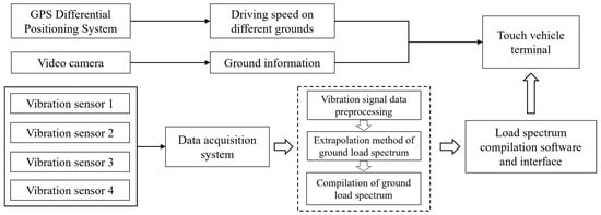
Figure 1.
Schematic diagram of the ground load acquisition system.
According to the national standard on road roughness GB7031-86 Vehicle Vibration Input Road Roughness Representation Method [33], the selected road surfaces for farming experiments have a wavelength range of 0.1–100 m. Considering the maximum possible speed of the tractor driving on various types of ground, the maximum excitation frequency of the road surface to the tire is calculated to be less than 100 Hz according to Equation (1):
The sampling frequency of the data acquisition should be at least four times the maximum excitation frequency of the road roughness to fully capture the tractor’s vibration acceleration. Hence, we use a 1 kHz sampling frequency in the load data acquisition system for the experiments.
2.2.2. Platform of the Experimental Tractor
In the experiments, the selected tractor is the Dongfanghong LX1404 (China YTO Group), which has specific parameters as shown in Table 2. Figure 2 demonstrates the installation of 4 vibration sensors for measuring the ground load data in the vertical (Z-) axis in Figure 2. The sensors are attached close to the wheel’s flange to ensure a straight and accurate vibration measurement. Figure 3 displays the data acquisition system’s hardware installed on the tractor. Vibration sensors 1 and 2 are installed on the tractor’s left and right front axles, respectively, and vibration sensors 3 and 4 are installed on the left and right rear axles. The sensors are sucked by strong magnets while adding shims to help level and ensure the measured vertical acceleration signals. The mobile GPS antenna is attached to the front hood of the tractor, and the GPS base station is erected on a tripod at a high place. The video camera is fixed to the front counterweight of the tractor to monitor and record different types of ground during the experiment. Moreover, the suction cup installs the touch vehicle terminal on the tractor cab side. Before the experiment, we calibrated the data acquisition instrument and vibration sensors using a standard 1 GHz acceleration instrument and debugged the real-time communication between the GPS reference station and the mobile station. We also used the acquisition software to check whether each parameter and signal of the entire detection system was running normally.
Table 2.
The specifications of the tractor in the experiment.
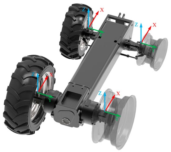
Figure 2.
Installation of four vibration sensors for measuring acceleration signals.
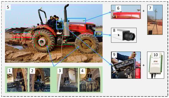
Figure 3.
The sensor installation diagram of the experimental tractor: 1. Vibration sensor for front axle (left), 2. Vibration sensor for front axle (right), 3. Vibration sensor for rear axle (left), 4. Vibration sensor for rear axle (right), 5. Experimental tractor, 6. GPS mobile station antenna, 7. GPS base station antenna, 8. Video camera, 9. Tractor touch vehicle terminal, 10. Vibration signal data acquisition system.
2.3. Acquisition System
Being different from the ground load of other vehicles, the ground load of the tractor vibration needs to include all the necessary ground conditions that a tractor may experience in regular transportation, as well as operating typical farm implements. The study considers six ground conditions of the test field: cement ground, hard soil ground, soft soil ground, sloped ground, ploughing ground, and rotary tillage ground, as shown in Figure 4. In the last two ground experiments, the tractor performs the farming operations. After the wheels roll, the rut formation can identify the hard and soft soil ground. The hard soil ground is mainly marked by shallow indentations, while the soft soil consists of fine soil and clods, marked by deep ruts covered with vegetation. The farm field uses soft soil ground for the vibration tests. The ploughing ground is the farm field after harvesting grains, and the rotary tillage ground for the test is the field after ploughing. The test field for each ground condition is 140 m in length and 3–5 lines in width. The tractor follows the driving speed listed in Table 3 to run the test field. In the ploughing test, the ploughing depth is about 25 cm.
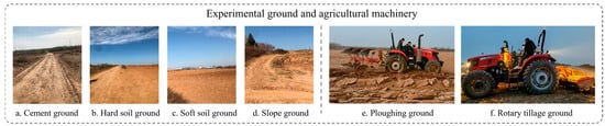
Figure 4.
Farm implements and the experimental ground sections.
Table 3.
Speed of different ground experiments.
3. Theory and Method
Figure 5 presents the theoretical basis with consistent steps for compiling the ground load spectrum of the whole tractor. Among the processes, the preprocessing section is essential for obtaining reliable acceleration load data. As shown, the process mainly includes three parts. First, there is a preprocessing section for dealing with the original ground load signals, including the welch power spectral density estimation of the six ground vibration loads, the CEEMDAN algorithm decomposition of the original signal, the wavelet threshold denoising algorithm, and the evaluation of the data denoising effect. Second, the study introduces a compilation method, including the time-domain extrapolation with the super-threshold model, GPD (Generalized Pareto Distribution) function, MEF (Mean Excess Function) threshold selection, and GPD parameter estimation. Third, the ground load spectrum is finalized for all ground testing and provides related software with multi-functions, including human–computer interaction, the visualization of real-time signal acquisition, data preprocessing display, and load spectrum compilation.
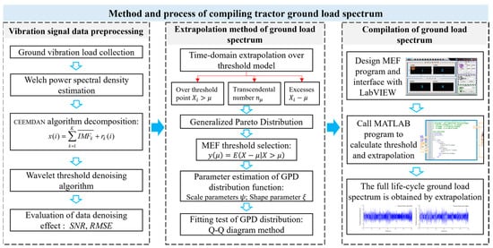
Figure 5.
Research on compiling method of tractor ground load spectrum.
3.1. Data Preprocessing Method
The ground vibration signal received by the tractor during driving has the characteristics of nonlinearity and non-stationary. In the process of data acquisition and transmission, vibration signals will be subject to different types of noise interference, including external ground environment interference, internal sensor uncertainties, and other hardware system errors [34], which will have a certain impact on the feature extraction and preprocessing analysis of acceleration signals. Therefore, it is necessary to denoise vibration signals and reduce abnormal points for ground load data preprocessing and load spectrum extrapolation.
(1) The CEEMDAN algorithm decomposition of the original signal
With regard to the acceleration signal processing problem, this paper adopts the Complete Ensemble Empirical Mode Decomposition with Adaptive Noise algorithm (CEEMDAN algorithm). The CEEMDAN algorithm decomposes the vibration signal into a series of intrinsic mode components (IMF) through the EMD algorithm and adds the idea of adaptive noise and multiple superposition in the EEMD method to reduce mode aliasing [35]. Then, the paper uses the wavelet threshold algorithm to denoise the high-frequency IMF components that carry more noise. The method aims to achieve a joint denoising effect and reduce the real information loss. The CEEMDAN method flowchart is shown in Figure 6.
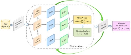
Figure 6.
The CEEMDAN method flowchart.
The CEEMDAN method is to add Gaussian white noise to the residual value every time the first order IMF component is calculated, calculating the mean value of the IMF component at this time, and iterating step by step. The process is as follows:
① Add Gaussian white noise w(i) of standard normal distribution to the collected original ground vibration signal x(i), perform J-times EMD decomposition of the newly generated signal, and repeat the overall average calculation of the generated modal component .
② Remove the residual of the first order component IMF1: .
③ Perform new EMD signal decomposition in r1(i) to obtain the first IMF1 component of the CEEMDAN decomposition. The second modal component and the residual r2(i) of the second order component are obtained by overall average calculation.
④ Repeat steps 2–3 until the residual signal obtained is a monotone function and the iteration cycle stops. Finally, K-times intrinsic modal components IMFk are obtained, and the original signal x(i) is decomposed into:
(2) Wavelet threshold denoising algorithm
The wavelet threshold denoising algorithm is used to reduce the order of IMF components of high-frequency noise through the Mallat tower algorithm, convert them into scale spaces of different scales, and obtain wavelet coefficients through threshold processing, filter and delete noise signals, and finally reconstruct signals. In this paper, the wavelet threshold is selected by the soft threshold function, where w is the wavelet coefficient and thr is the threshold.
Wavelet denoising soft threshold function expression is:
(3) Evaluation of data denoising effect
Reconstruct the processed signal components to obtain the complete signal after denoising. Through the comparative analysis of the waveform and spectrum before and after signal processing, the visual signal denoising effect is obtained. The preprocessing effect is measured by calculating the Signal Noise Ratio (SNR) and Root Mean Square Error (RMSE) of the vibration signal.
The SNR calculation formula is:
The RMSE calculation formula is:
where is the original vibration signal and is the processed signal. The smaller RMSE and the larger SNR indicate that the denoising effect of this method is better. Finally, the wavelet threshold denoising process is shown in Figure 7.
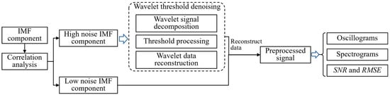
Figure 7.
Flow chart of wavelet threshold denoising.
3.2. Time-Domain Extrapolation Method of Ground Load
The load extrapolation method plays a vital role in the load spectrum compilation. The load extrapolation methods can be categorized as rainflow basin extrapolation and time-domain extrapolation. Skipping the rainflow counting steps, one can directly extrapolate a new ground load time series from the measured data while preserving the time history of the data to a great extent [36]. Therefore, after the CEEMED and wavelet threshold denoising algorithms preprocess the original data, we develop a comprehensive process of spectrum compilation based on the time-domain extrapolation method. Due to the ground load intensity and complexity, we establish a POT model-based time domain extrapolation method and complete several tasks as follows: establish an extreme value sampling model of POT; obtain the GPD function and estimate its parameters; select the threshold by the MEF method and complete the fitting test of the GPD. To be noted, the paper conducts the fitting of the GPD function to find the distribution features of the measured ground vibration load. Since the selection of the load threshold can greatly affect the amount of data over the threshold, it is crucial to determine a reasonable threshold range for ensuring high accuracy and fast computing speed. After determining all the extrapolation steps, we will further embed it in our developed software for generating the ground load spectrum. The following describes the specific details for each task:
(1) Establishment of extreme value sampling model of POT.
In the POT model, the selected data are the samples within specific extreme values (between the upper and lower thresholds). represents the ground vibration load data measured from the tractor’s front and rear axles. Each sample is a time series and has n random ground load data independent of each other while coming from the same distribution function F(x). represents the threshold. The data greater than () are the super-threshold data with the excess . Moreover, the corresponding super-threshold distribution function can be obtained as follows:
(2) Generalized Pareto Distribution
Since the ideal distribution function is unknown, the study analyzes the distribution of super-threshold data and the data amount to optimize and obtain a conditional distribution function. According to the theory, the super-threshold distribution is asymptotically distributed when the threshold is sufficiently large, which brings the GPD. Generally, the cumulative distribution function and the probability density function are used to describe the GPD, which can be expressed by Equations (7) and (8):
According to extreme value theory, if a random time series of loading sets has the characteristics of a fat tail, the excess of this dataset can be viewed as the GPD.
(3) Estimate parameters of GPD function
The research shows that it is more effective and consistent using the MLE method to find the solutions in the GPD function [37]. The present paper adopts the MLE method for solving the GPD function and solves the scale parameter and shape parameter . The details are shown as follows:
① When , the likelihood function is solved by taking the logarithm on both sides of the GPD function and gets:
By taking the partial derivatives of and and applying the Newton iteration method, Equation (9) is solved to obtain the likelihood estimates of and .
② When , the logarithm form of the likelihood function for the GPD function is expressed as:
Taking the partial derivative of on Equation (10) gets:
(4) The MEF threshold selection method
In the POT extreme value model, the threshold determines the quality of the fitting of the GPD function. If the selected threshold is too small, more super-threshold points will remain in the data sample, causing computation waste. If the selected threshold is too large, the obtained random data are deficient in fully reflecting the distribution features, causing poor accuracy. To find an appropriate threshold, we employ a graphical method with the use of the MEF method. According to the principle of the GPD, when the load data obey the GPD function , the distribution of the obtained data obeys the GPD function , where is the threshold. The average excess distribution function of the obtained data is expressed by Equation (12).
When determining appropriate parameters and and obtaining the corresponding GPD function, the averaged excess distribution function is linear to the selected threshold . In the MEF diagram, the region closest to the fluctuation area ensures the linear relationship between the averaged excess and the threshold . In this region, the relation expression between the average excess value and the threshold value is as follows:
Therefore, a threshold in the linear region of the MEF diagram is chosen as the optimal upper threshold for the GPD fitting.
(5) Goodness-of-fit test for GPD distribution
As discussed above, the extrapolated method finds the suggested scale and shape parameters , obtains the load data threshold, and then fits the extreme value data. However, the applicability and goodness of fitting the GPD is unclear. This task uses the Q-Q diagram method to assess the fitting effect and verify the proposed threshold.
After obtaining the distribution function, we obtain its uniformed distribution function over the interval (0, 1). represents the order statistic of the random time series and the uniformed distribution function can be expressed as:
Next, this study plots the Q-Q diagram for the extreme value data using the following equation:
This paper also draws a straight line of the selected distribution function on the Q-Q diagram to judge the quality of fitting the GPD. When the data points are close to the proposed line, the fitting agrees well with the original GPD.
3.3. Extrapolation Process of Ground Load Spectrum
After validating the suggested threshold with the goodness-of-fit for the GPD, we can extrapolate the selected sample following the steps shown in Figure 8.
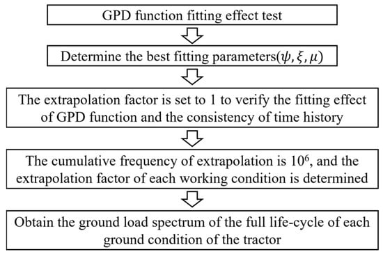
Figure 8.
Ground load spectrum extrapolation flowchart.
4. Results and Discussion
4.1. Data Collection and Preprocessing
4.1.1. Experimental Data Collection
Figure 9 provides the temporal curve of the rear axle (right) data with respect to different ground conditions. When the tractor runs on cement ground and hard soil ground, the corresponding data amplitude is lower than that of soft soil ground and slope ground due to the better ground flatness. Besides, the signals demonstrate a significantly higher amplitude and more severe fluctuations in the ploughing ground and rotary tillage ground experiments. Especially, the signal amplitude during the rotary tillage is the highest due to the reduction of ground smoothness and the addition of uneven-sized soil blocks after ploughing.
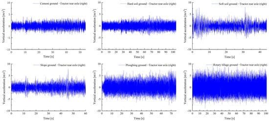
Figure 9.
Tractor rear axle (right) data curve for six kinds of ground.
Figure 10 shows the power spectral density (PSD) analysis of the rear axle (right) data under different ground conditions, using the Rectangular Window Welch method to describe the change of energy characteristics of vibration signals with frequency. It can be seen from the figure that, under different ground conditions, the vibration energy of most signals is concentrated in low frequency and high frequency areas. The cement ground is relatively stable, and its energy is concentrated in the middle and low frequency areas. The vibration data other than cement ground demonstrate a similar curve. However, their curves indicate that the intermediate frequency region possesses high energy components, which will cause interference to the feature parameter extraction in the following process. The processing of the denoising is thus required and necessary to eliminate the useless information from the vibration signals.
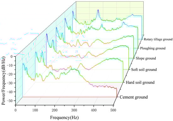
Figure 10.
Welch power spectral density estimation of six ground vibration loads.
4.1.2. Load Data Preprocessing
As discussed in the last section, the CEEMDAN algorithm is used to decompose the original vibration signal x(i). Taking the ploughing process of the tractor as an example, we use its vibration data of the rear axle (right) for presenting the effect of decomposition and denoising. In the acquisition, the sampling frequency of the signal is 1000 Hz, and the data length is 75,000. For the decomposition, the standard deviation of adding Gaussian white noise to the signal is 0.2, the average number of times of adding noise is 100, and the maximum number of iterations of the signal is set to 5000. Figure 11 shows that the CEEMDAN modal decomposition diagram has 19 IMF (IMF 1~IMF 19) frequencies from high to low.
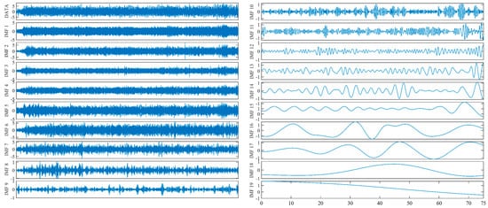
Figure 11.
The CEEMDAN decomposition results. Note: X−axis: Time (s), Y−axis: Vibration acceleration (m·s−2).
The Permutation Entropy algorithm (PE) is used to quantitatively evaluate the random noise contained in the signal sequence, which is used as the judgment basis for the high noise IMF component and the effective IMF component [38]. We calculate the PE value of each modal component IMF, as shown in Table 4. Next, a PE value of 0.5 is selected as the judgment threshold. When PE > 0.5, the corresponding IMF components are subject to wavelet denoising, and the other IMF components are retained. From the table, the PE values of IMF 1~IMF 7 are greater than 0.5, which indicates that the noise content is high. According to the verification and analysis, the first seven IMF components are subject to wavelet denoising.
Table 4.
The PE value of IMF components.
Next, the study employs the wavelet soft threshold denoising algorithm to denoise the IMF component data. The denoised vibration signal of the right rear axle for ploughing is reconstructed and shown in Figure 12, Besides, the corresponding vibration signal without denoising is also provided for comparison. In the figure, the overall amplitude of the denoised signal is decreased while the peaks have the same amplitude as the original signal. The processed signal denotes a reduction of the signal interference, effectively filtering the noise while retaining the true signal. As shown in Table 5, the denoising effect during preprocessing is measured by calculating the SNR and RMSE of the original vibration signal and the noise-reduced signal [39] to compare the three denoising methods used in the processing: 3σ-rule denoising, wavelet hard threshold denoising, and wavelet soft threshold denoising. The SNR after wavelet soft threshold denoising is relatively larger and the RMSE is smaller, which effectively reduces the high noise of the original signal, provides cleaner data for the preparation and extrapolation of the load spectrum of the ground vibration signal, and helps improve the accuracy and reliability of the load spectrum.
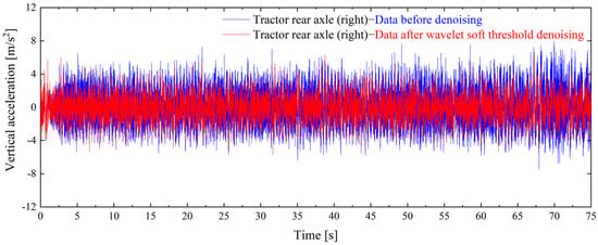
Figure 12.
Comparison before and after data denoising.
Table 5.
Effect comparison of different denoising methods.
4.2. Ground Load Spectrum Compilation and Extrapolation
Figure 13 plots the MEF diagram of the ploughing ground load data and demonstrates how the estimated mean excess varies with respect to the upper limit threshold value. Note that the lower threshold value is negative due to the opposite vibrating direction. As shown in the figure, the curve has a sharp decrease before the upper threshold reaches 0.5 m·s−2, and then gradually decreases with the increase in the upper threshold. Finally, the curve severely fluctuates when the upper threshold is higher than 4.2 m·s−2. As the threshold selection principle suggests, the region close to the beginning of the fluctuation usually has a linear relationship between the mean excess and the threshold. The optimal upper threshold can thus be picked in this region to ensure the quality of the fitting of the GPD. Figure 13 also presents the zoomed area prior to the fluctuation. The red line in the zoomed diagram denotes the linear relationship referring to the suggested function. The diagram verifies that the curve is very close to the red line, suggesting its good linearity. Therefore, an optimal upper threshold of μu = 4.152 m·s−2 is determined. Repeating such a method, we quickly obtain all the upper and lower thresholds of the four axle loads under all the ground conditions.
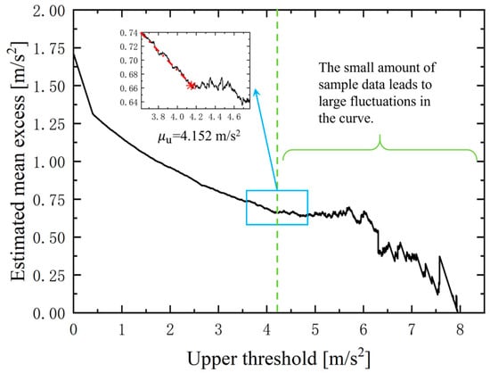
Figure 13.
The MEF diagram of the excess of the upper limit threshold of the ploughing ground load.
The study uses the maximum likelihood estimation Equations (9)–(11) to find the GPD parameters for the excess data after getting the optimal threshold value. Table 6 lists the corresponding results, including the calculated threshold, the shape parameter, and the scale parameter.
Table 6.
Fitting results of GPD distribution parameters for ploughing process data.
With the parameters provided in Table 6, the different POT models of the processed ground load data of the four axles are obtained. For instance, the bi-directional POT model for the load data on the tractor’s rear right axle is expressed by the upper and lower thresholds, respectively. For the upper threshold of the positive-directional vibration, the best-fitted GPD function of the POT model is:
For the lower threshold of the negative-directional vibration, the best-fitted GPD function of the POT model is:
Performing the mentioned steps obtains all the fitted GPD functions for the different ground load data of the different tractor axles. Next, the study follows Equation (15) and plots the Q-Q diagram to visually examine the effect of fitting the corresponding GPD. For instance, we plot the Q-Q diagram (Figure 14) for the rear right axle load of the ploughing ground. Based on the principle, a proper fitting features a typical fat-tailed shape of the scatter (sample data quantile vs. expected normal quantile) distribution. The figure shows that the fitted data (as marked by pink crosses) greatly fit the reference line in the middle area while deviating from the line at the two ends. Besides, the slight deviation denotes that the points roughly agree with the proposed line. Therefore, the Q-Q diagram suggests an appropriate fitting for the selected GPD functions.
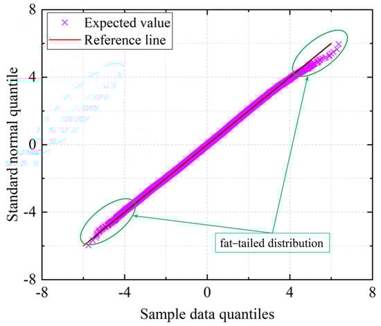
Figure 14.
The GPD-fitted Q-Q plot of ploughing ground.
The next step is determining the extrapolation factor to derive an appropriate ground load spectrum. The time-domain extrapolation method requires extrapolating the ground load data n times of the GPD probability density and cumulative distribution functions. According to previous studies, the cycle frequency of the rainflow counting matric should be up to 106 times in order to contain all the possible loads [40]. Therefore, the present study adopts the number of cycles of 106 as a criterion to determine the extrapolation factor for getting a full life-cycle load spectrum.
Figure 15 provides several generated load spectra by extrapolating different times on the ploughing load data of the tractor’s rear right axle. As shown in the figure, when the extrapolation factor equals 1, the generated load sample has the same size and cumulative number of cycles as the original sample (after denoising). The increase in the extrapolation factor leads to an apparent increase in the cumulative number of cycles. After consistent numerical computations, we find the cumulative cycle number reaches 106 times when the extrapolation factor is 287. Therefore, the extrapolation factor of 287 is determined and used for producing the ploughing ground load spectrum. Figure 16a,b present the extrapolated ground load spectrum for the extrapolation factors being 1 and 287, respectively. The original load data are also plotted in Figure 16a. Compared to the original sample, the 1-time extrapolated load spectrum is similar but slightly different. The difference demonstrates how preprocessing and extrapolation change on the original sample. When extrapolated 287 times, the generated load spectrum becomes much more intensive than the original one. The study further employs the analysis of the processed ground load spectra for validation.
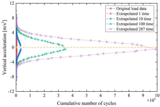
Figure 15.
Loading cycle frequency curve of different extrapolation factors.
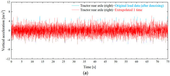
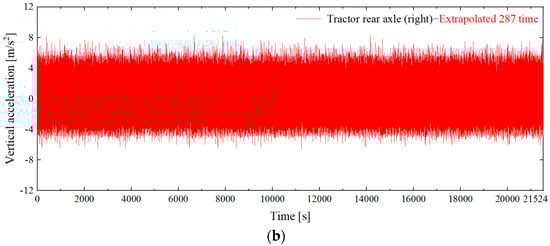
Figure 16.
Load data comparison curve: (a) Comparison of original load and extrapolated 1-time load spectrum; (b) Ground load spectrum extrapolated to the full life-cycle.
4.3. Correctness Inspection of Ground Load Spectrum Compilation
To assess the extrapolated ploughing ground load spectrum, this paper compares and analyzes the extrapolated results with the original data in two aspects, statistical and rainflow counting. The statistical analysis compares the maximum value, mean value, standard deviation, and variance to reveal the statistical features. The rainflow count analysis reflects the magnitude and cycle frequency features. Since it can efficiently explore the inherent characteristics of the actual load cycles, rainflow counting is usually applied in the fatigue damage evaluation. The study presents two analyses on different ground load spectra before and after the extrapolation. Still, it employs the ploughing ground load data for the tractor’s rear right axle to keep consistency with the above examples.
Table 7 shows the statistical parameters of the original and extrapolated data. Besides, the extrapolated load data with different extrapolation factors are considered. As seen in the table, the extreme value of the load data increases with larger extrapolation factors. After extrapolating 287 times, both the maximum and minimum amplitude are extrapolated. Specifically, the extreme value range has expanded from (−5.926, 6.438) to (−6.223, 6.736), and the ground load coverage is increased by 4.81%. At the same time, the mean, standard deviation, and variance values before and after the extrapolation are similar without any significant change. From a statistics perspective, the extrapolation keeps the characteristics of the original data and effectively expands the load amplitude and ground load coverage. Hence, the extrapolation mimics the original loading behavior while allowing for higher extreme loads in fatigue than the largest measured ones.
Table 7.
Statistical characteristics of extrapolated data of rear axle (right) load during ploughing.
The paper also investigates the rainflow counting analysis on the original and extrapolated load spectra. Aiming to reveal the similarity, this paper compares the original load (after denoising) spectrum with the 1-time extrapolation, which has the same load time histories. Figure 17 separately derives the load cycles versus mean and amplitude histograms to perform a correlation analysis. All the spectrum distributions after 1-time extrapolation present similar behaviors to that of the original data. To further investigate the correlation between the extrapolation and the original data, we calculate the correlation coefficients for each histogram. The results show that the correlation coefficient for the load mean histogram is 0.968, and the one for the load amplitude is 0.989. The rainflow counting matrices in Figure 18a,b also observe a high correlation. When extrapolating the data up to 287 times, their rainflow counting matrix in Figure 18c looks similar to the matrix in Figure 18a. This analysis indicates that such an extrapolation keeps the load characteristics of the original data. There are still some differences between the two matrices. The extrapolated one (extrapolating 287 times) presents not only an expansion in the mean and amplitude, but also a high number of cycles. Consequently, this analysis proves that the proposed time-domain extrapolation is applicable and effective in obtaining different ground load spectra for reproducing a longer period of the tractor’s vibration. In addition, in a future fatigue test of a four-poster rig for the tractor, instead of applying the largest measured load, the extrapolation allows for more extreme cycles with higher amplitude.
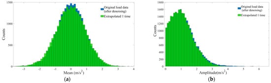
Figure 17.
Comparison of Mean and Amplitude counts of original load and extrapolated 1-time load data: (a) mean counts histogram; (b) amplitude counts histogram.
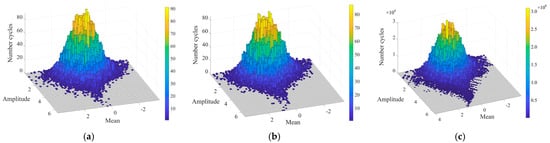
Figure 18.
Comparison of rainflow count matrices for load data: (a) Original load (after denoising) rainflow matrix, (b) Extrapolated 1-time rainflow matrix, (c) Extrapolated full life-cycle rainflow matrix.
5. Conclusions
To improve the ability of indoor tractor vibration testing on a four-poster rig, this paper proposed a data acquisition and spectrum compilation method for generating a full life-cycle load spectrum. To avoid overestimating the vibration and reproduce real-world ground profiles, this research considered the tractor’s actual working and transportation scenarios by properly incorporating different ground excitations that the tractor meets daily. This paper measured the tractor’s load vibration signals under six ground conditions: cement ground, hard soil ground, soft soil ground, slope ground, ploughing ground, and rotary tillage ground. Using a developed data acquisition system, we obtained all the vertical vibration signals of the tractor’s front and rear axles. Afterward, this paper used Welch power spectral density estimation and the CEEMDAN algorithm to decompose the original signal and utilized the Wavelet threshold denoising algorithm to denoise the original ground load signal. Additionally, a unified time-domain extrapolation method was investigated based on the study of the POT super-threshold model, POT sampling principle, threshold value selection by MEF curve, parameter estimation by GPD function, and the goodness-of-fit test for GPD function. After a series of correction analyses, the extrapolated ground load spectra were eventually determined with appropriate extrapolation factors.
The statistical analysis on the extrapolated ploughing-ground load spectrum of the tractor’s rear right axle demonstrates an enhancement. After the extrapolation, the extreme value range of data expanded from (−5.926, 6.438) to (−6.223, 6.736), and the ground load coverage increased by 4.81%. Other statistic parameter analyses (mean, standard deviation, and variance) indicated a similar behavior of the extrapolated load spectrum to the original ones. The rainflow counting analysis verified a high correlation between the 1-time extrapolation and the original data, in which the correlation coefficients for the load mean- and amplitude-histograms were 0.968 and 0.989, respectively. As shown in the analysis of the rainflow counting matrices, the load spectrum extrapolation demonstrated a similar behavior meanwhile, amplifying the mean and amplitude, as well as the number of cycles. These results validated that the extrapolation is capable of preserving the measured load characteristics to the fullest extent while enhancing the signal quality to some extent. Finally, the unified full life-cycle ground load spectrum consisting of six ground conditions and different farming operations was obtained.
In summary, the edited ground load spectrum is appropriate for comprehensively combining actual ground loads. Meanwhile, the unified study on tractor vibration data acquisition, data preprocessing, and load spectrum extrapolation was verified to reproduce complete and extrapolated load information effectively. However, more studies are required to figure out the correlations between environmental factors and tractor vibration. These are essential works for quantifying the reasons for reducing tractor fatigue and durability and finding the representative environmental factors. In the future, this study will also make more efforts to employ the proposed load spectrum on the four-poster rig for testing.
Author Contributions
Conceptualization, S.W.; methodology, D.D.; software, D.D.; validation, D.D. and S.L.; investigation, D.D. and S.L.; resources, X.M., D.C. and B.Z.; data curation, D.D. and S.L.; writing—original draft preparation, D.D.; writing—review and editing, D.D. and X.M.; project administration, X.M., Z.M., D.C. and Z.W. All authors have read and agreed to the published version of the manuscript.
Funding
This work was financially supported by Jiangsu Province and Education Ministry Co-sponsored Synergistic Innovation Center of Modern Agricultural Equipment (XTCX2005, XTCX2011), the National Natural Science Foundation of China (32201687), and National Key Research and Development Program of China (Grant No. 2016YFD0700102).
Institutional Review Board Statement
Not applicable.
Data Availability Statement
The data presented in this study are available on demand from the first author at daidong_zb@cau.edu.cn.
Acknowledgments
The authors thank the Jiangsu Province and Education Ministry Cosponsored Synergistic Innovation Center of Modern Agricultural Equipment (XTCX2005, XTCX2011) and National Key Research and Development Program of China (Grant No. 2016YFD0700102) for funding.
Conflicts of Interest
The authors declare no conflict of interest.
References
- Mattetti, M.; Maraldi, M.; Sedoni, E.; Molari, G. Optimal criteria for durability test of stepped transmissions of agricultural tractors. Biosyst. Eng. 2019, 178, 145–155. [Google Scholar] [CrossRef]
- Zhao, C. Analysis of tractor product characteristics and development trend at home and abroad. Tract. Farm Transp. 2021, 48, 1–9+15. [Google Scholar]
- Hostens, I.; Anthonis, J.; Kennes, P.; Ramon, H. PM—Power and Machinery: Six-degrees-of-freedom test rig design for simulation of mobile agricultural machinery vibrations. J. Agric. Eng. Res. 2000, 77, 155–169. [Google Scholar] [CrossRef]
- Li, M.; Yang, Q.; Chen, J. Design of tractor vibration testing system. J. Northwest AF Univ. (Nat. Sci. Ed.) 2010, 38, 229–234. [Google Scholar]
- Abubakar, M.S.; Ahmad, D.; Akande, F.B. A review of farm tractor overturning accidents and safety. Pertanika J. Sci. Technol. 2010, 18, 377–385. [Google Scholar]
- Wang, B. Cause analysis and preventive measures of agricultural machinery vibration. Farm Mach. Using Maint. 2014, 2, 26. [Google Scholar]
- Zhang, W.; Zhang, W.; Lu, Z.; Wang, B.; Tong, B. Research of wheeled tractor roll stability based on virtual prototyping technology. J. Mech. Strength 2017, 39, 138–142. [Google Scholar]
- Mattetti, M.; Molari, G.; Vertua, A. New methodology for accelerating the four-post testing of tractors using wheel hub displacements. Biosyst. Eng. 2015, 129, 307–314. [Google Scholar] [CrossRef]
- Tucker, L.; Bussa, S. The SAE cumulative fatigue damage test program. In SAE Technical Paper; 750038; SAE: Warrendale, PA, USA, 1975; pp. 1–51. [Google Scholar]
- Molari, G.; Mattetti, M.; Falagario, A.; Sedoni, E. Tractor accelerated structural testing by means of the rainflow method. In Solutions for Intelligent and Sustainable Farming; VDI: Düsseldorf, Germany, 2011; pp. 217–222. [Google Scholar]
- Chindamo, D.; Gadola, M.; Marchesin, F.P. Reproduction of real-world road profiles on a four-poster rig for indoor vehicle chassis and suspension durability testing. Adv. Mech. Eng. 2017, 9, 1–10. [Google Scholar] [CrossRef]
- Zou, C. Research on the application of four column vibration table in vehicle fatigue test. Auto Parts 2018, 11, 142–144. [Google Scholar]
- Li, S.; Li, Y.; Ma, L. Research on road simulation test of electric vehicle. Automob. Technol. 2017, 02, 16–19. [Google Scholar]
- Shen, J.; Chen, Y.; Hu, H.; Xu, W.; Wang, W. Development of road simulation test for lower control arm on passenger cars. Chin. J. Automot. Eng. 2017, 1, 66–71. [Google Scholar]
- Duan, H.; Shi, F.; Xie, F.; Zhang, K. Summary of research on road spectrum measurement. J. Electron. Meas. Instrum. 2010, 24, 72–79. [Google Scholar] [CrossRef]
- Yan, J.G.; Wang, C.G.; Xie, S.S.; Wang, L.J. Design and validation of a surface profiling apparatus for agricultural terrain roughness measurements. R D Natl. Inst. Agric. Food Ind. Mach.-INMA Buchar. 2019, 59, 169–180. [Google Scholar] [CrossRef]
- Schiehlen, W.; Hu, B. Spectral simulation and shock absorber identification. Int. J. Non-Linear Mech. 2003, 38, 161–171. [Google Scholar] [CrossRef]
- Perera, R.W. Certification of Inertial Profilers. In Proceedings of the International Conference on Highway Pavements and Airfield Technology 2017, Philadelphia, PA, USA, 27–30 August 2017; pp. 268–278. [Google Scholar]
- Gillespie, T.D.; Sayers, M.W.; Segel, L. Calibration of response-type road roughness measuring systems. In NCHRP Report; Transport Research Board: Washington, DC, USA, 1980; pp. 1–290. [Google Scholar]
- Han, S.B. Measuring displacement signal with an accelerometer. J. Mech. Sci. Technol. 2010, 26, 1329–1335. [Google Scholar] [CrossRef]
- Huang, J. Research on Pavement Spectrum Test of Hillside Tractors and Its Reappearance Method. Master Dissertation, Jilin University, Changchun, China, 2018. [Google Scholar]
- Ma, R.; Song, H.; Lai, X. Pavement roughness measurement system based on laser displacement sensors. J. Chang. Univ. (Nat. Sci. Ed.) 2006, 26, 38–41. [Google Scholar]
- Lu, Z.; Jin, W.; Jin, F.; Jiang, C.; Liu, Y.; Xu, H.; Wang, Z. Design and test of non-contact laser surface roughness instrument. J. Nanjing Agric. Univ. 2015, 38, 511–516. [Google Scholar]
- Luan, S.; Yu, J.; Zheng, S. Vehicle load correlation analysis method and optimization application of road simulation test. Mech. Sci. Technol. Aerosp. Eng. 2021, 40, 1944–1951. [Google Scholar]
- Londhe, A.; Kangde, S.; Karthikeyan, K. Deriving the compressed accelerated test cycle from measured road load data. In SAE Technical Paper; SAE: Warrendale, PA, USA, 2012; pp. 1–12. [Google Scholar]
- Ge, S.; Han, C. Investigation of equivalent load spectrum for simulation test of whole tractor. J. Anhui Inst. Technol. 1990, 9, 71–77. [Google Scholar]
- Kim, D.C.; Ryu, I.H.; Kim, K.U. Analysis of tractor transmission and driving axle loads. Trans. ASAE 2001, 44, 751–757. [Google Scholar]
- Mattetti, M.; Molari, G.; Sedoni, E. Methodology for the realisation of accelerated structural tests on tractors. Biosyst. Eng. 2012, 13, 266–271. [Google Scholar] [CrossRef]
- Wang, Y.; Wang, L.; Zong, J.; Lv, D.; Wang, S. Research on loading method of tractor pto based on dynamic load spectrum. Agriculture 2021, 11, 982. [Google Scholar] [CrossRef]
- Yang, Z.; Song, Z.H.; Zhao, X.Y.; Zhou, X.X. Time-domain extrapolation method for tractor drive shaft loads in stationary operating conditions. Biosyst. Eng. 2021, 210, 143–155. [Google Scholar] [CrossRef]
- Pan, H.; Liu, J.; Wang, N.; Zhao, J. Development of on-line monitoring equipment for tractor reliability test. Tract. Farm Transp. 2021, 48, 35–36. [Google Scholar]
- Li, J.; Sun, S.; Leng, J.; Zhang, Y. Research on frequency domain vibration fatigue acceleration testing of tractor hood based on damage equivalence. Agric. Equip. Veh. Eng. 2019, 57, 223–225. [Google Scholar]
- GB/T 7031-1986; Vehicle Vibration—Describing Method for Road Surface Irregularity. National Bureau of Statistics of China: Beijing, China, 1987; pp. 1–16.
- Duan, H.; Xie, F.; Zhang, K.; Ma, Y.; Shi, F. Methods of signal pre-processing with massive road surface measurement data. J. Vib. Shock 2011, 30, 101–106. [Google Scholar]
- Fei, H.; Shan, J. Application of CEEMDAN-Wavelet Threshold Method in the Signal Processing of Blasting Vibration. Blasting. 2022, 3, 41–47. [Google Scholar]
- Wang, Y.; Wang, L.; Wen, C.; Lv, D.; Wang, S. Extrapolation of tractor PTO torque load spectrum based on automated threshold selection with FDR. Trans. Chin. Soc. Agric. Mach. 2021, 52, 364–372. [Google Scholar]
- Wang, P.; Sun, H.; Chen, J.; Zhang, M.; He, C. Selection of time domain extrapolation GPD estimation method in super-threshold model. Chin. Hydraul. Pneum. 2021, 45, 38–43. [Google Scholar]
- Zhang, Z.; Liu, M.P.; Zhang, Z.T.; Wang, Q.N. A new method for power quality disturbance signal denoising based on CEEMDAN and wavelet soft threshold. Mod. Electron. Tech. 2021, 44, 63–68. [Google Scholar]
- Gu, Z. Research on Tracked Vehicle Engine Support Test System. Master Dissertation, North University of China, Taiyuan, China, 2020. [Google Scholar]
- Zhang, Y.; Wang, G.; Wang, J.; Hou, X.; Zhang, E.; Huang, J. Load spectrum compiling and fatigue life prediction of wheel loader axle shaft. J. Jilin Univ. Eng. Technol. Ed. 2011, 41, 1646–1651. [Google Scholar]


Disclaimer/Publisher’s Note: The statements, opinions and data contained in all publications are solely those of the individual author(s) and contributor(s) and not of MDPI and/or the editor(s). MDPI and/or the editor(s) disclaim responsibility for any injury to people or property resulting from any ideas, methods, instructions or products referred to in the content. |
© 2023 by the authors. Licensee MDPI, Basel, Switzerland. This article is an open access article distributed under the terms and conditions of the Creative Commons Attribution (CC BY) license (https://creativecommons.org/licenses/by/4.0/).