
Segmentation and Stratification Methods of Field Maize Terrestrial LiDAR Point Cloud

Abstract
:1. Introduction
- Go deep into the farmland and use reliable methods to complete the collection, registration, and cropping of field maize point clouds;
- Explore and verify, based on 3D laser point cloud technology, the spatial morphological characteristics of field maize;
- Create an individual maize segmentation model that can automatically identify and segment each maize plant from the scanned point cloud of the maize field;
- Create a maize organ stratification model that can accurately segment and visualized all maize organs from the field maize point cloud.
2. Materials and Methods
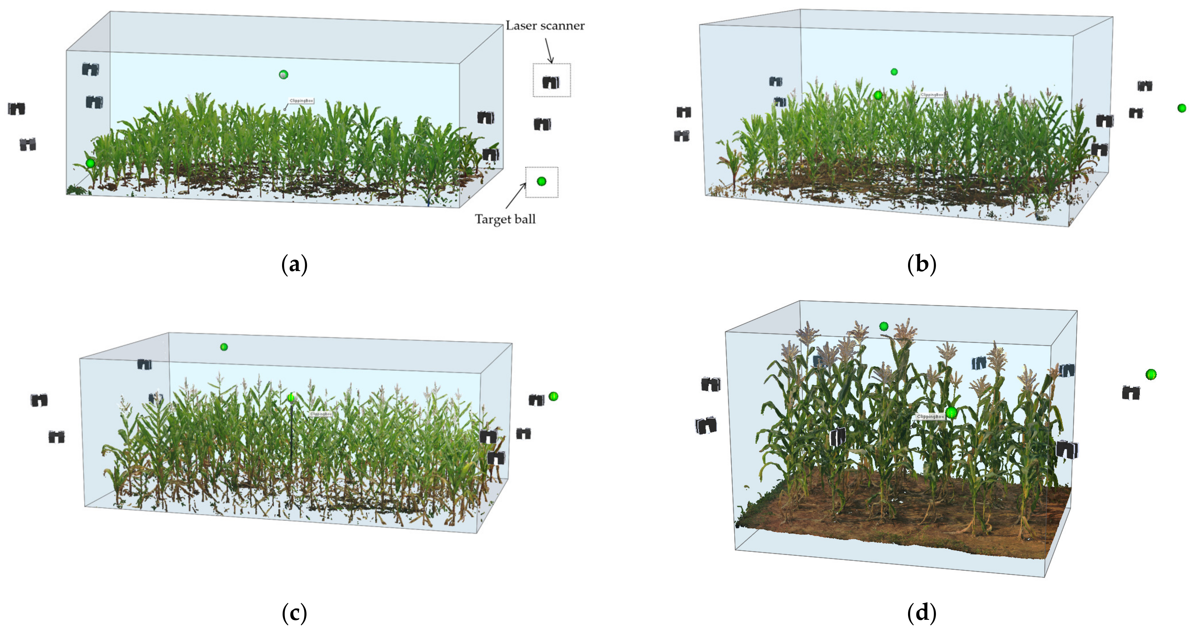
2.1. Material
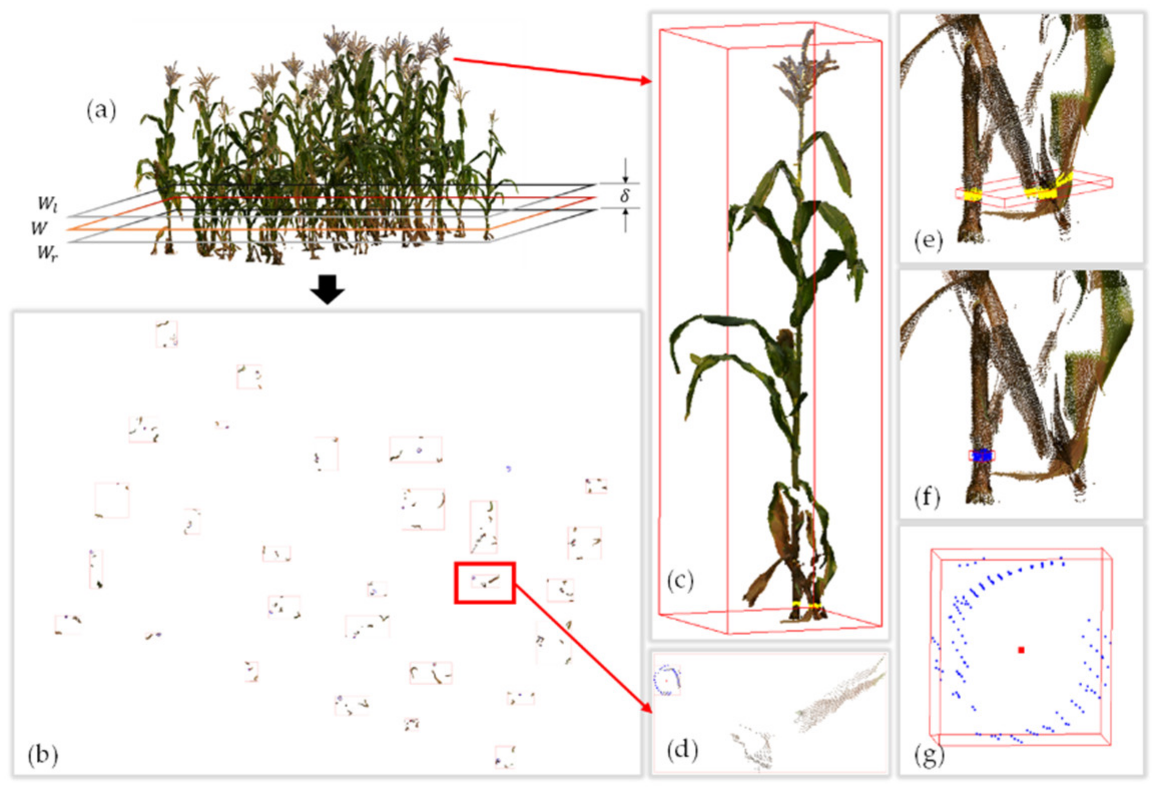
2.2. Individual Maize Segmentation Model
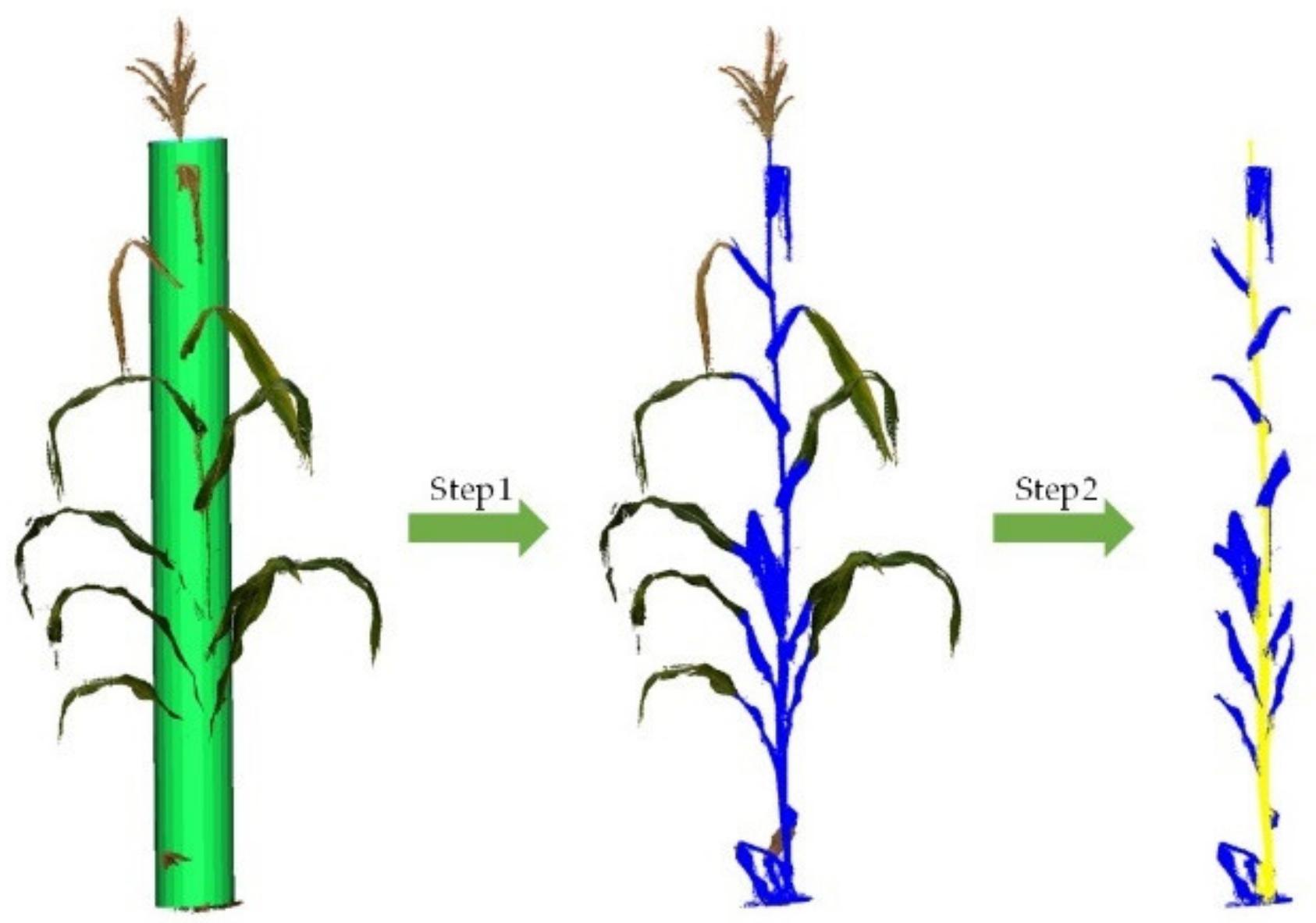
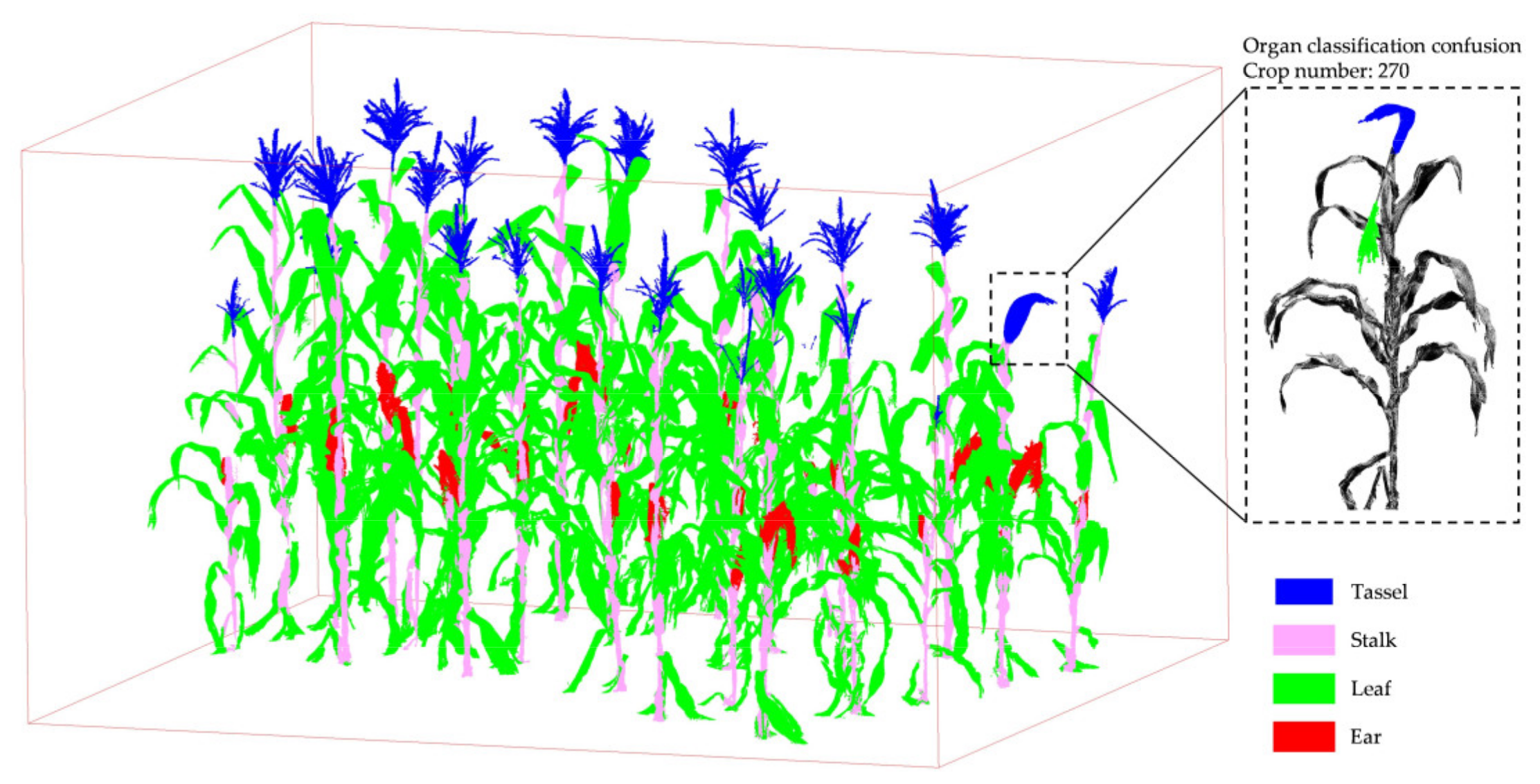
2.3. Maize Organ Stratification Model
- Stem segmentation
- 2.
- Identification of ear point sets
- 3.
- Identification of tassel and leaf point sets
2.4. Model Evaluation Metrics
3. Results and Discussion
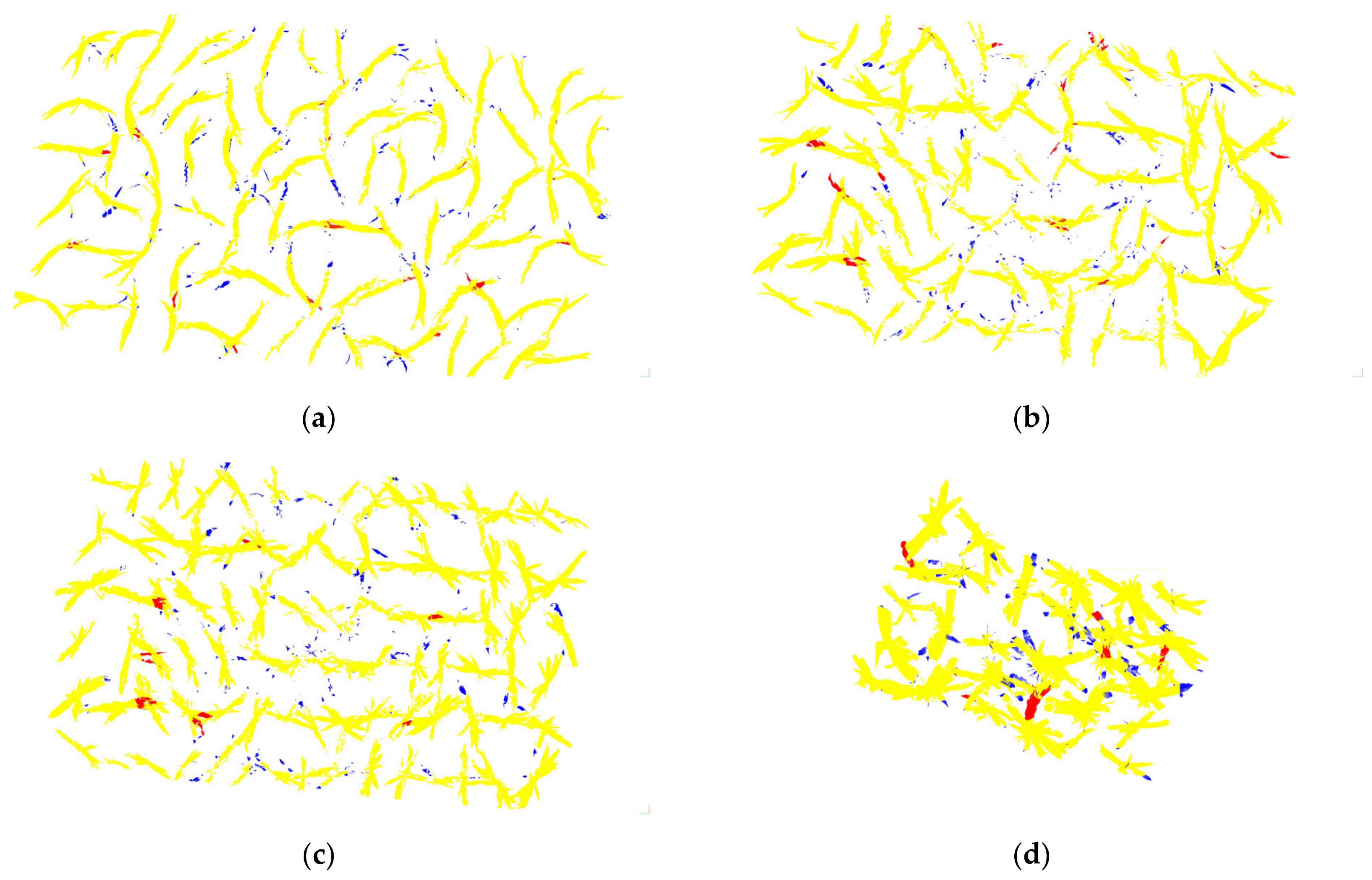
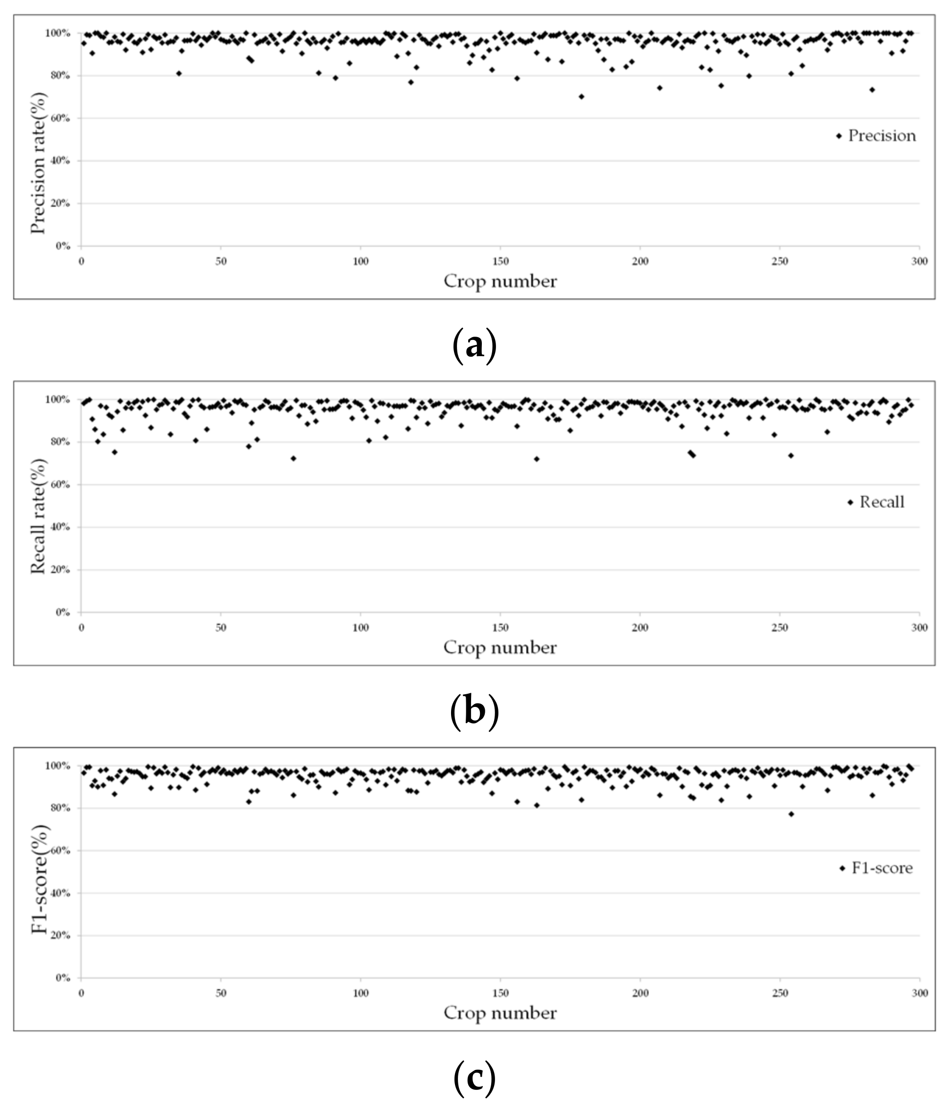
3.1. Segmentation Results and Analysis
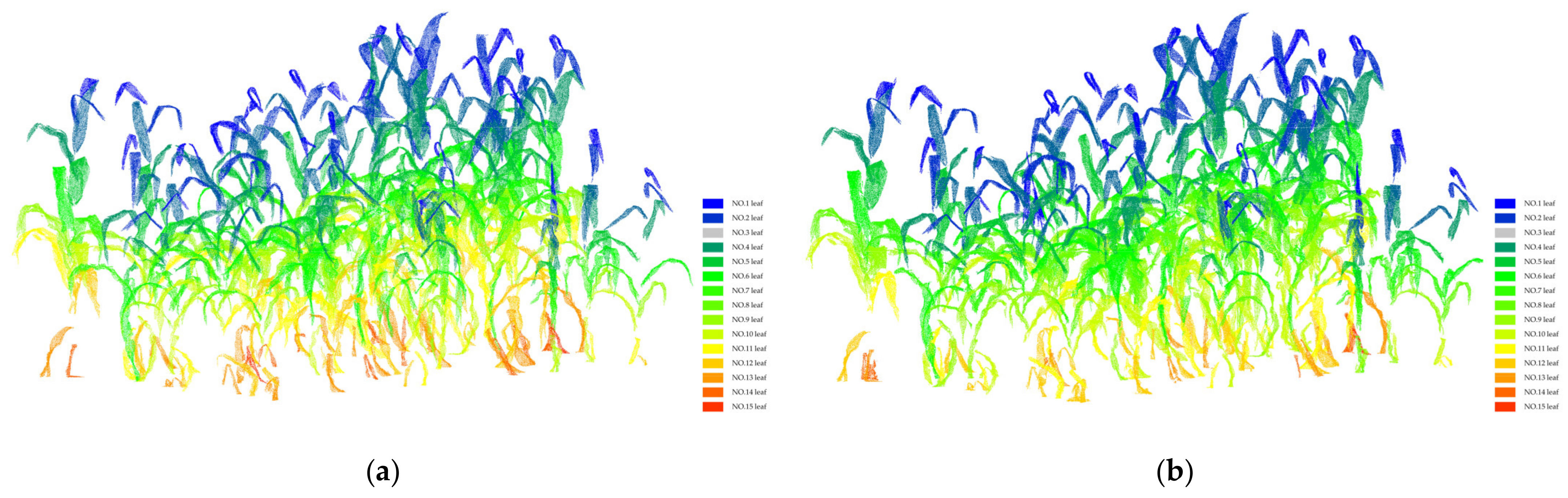
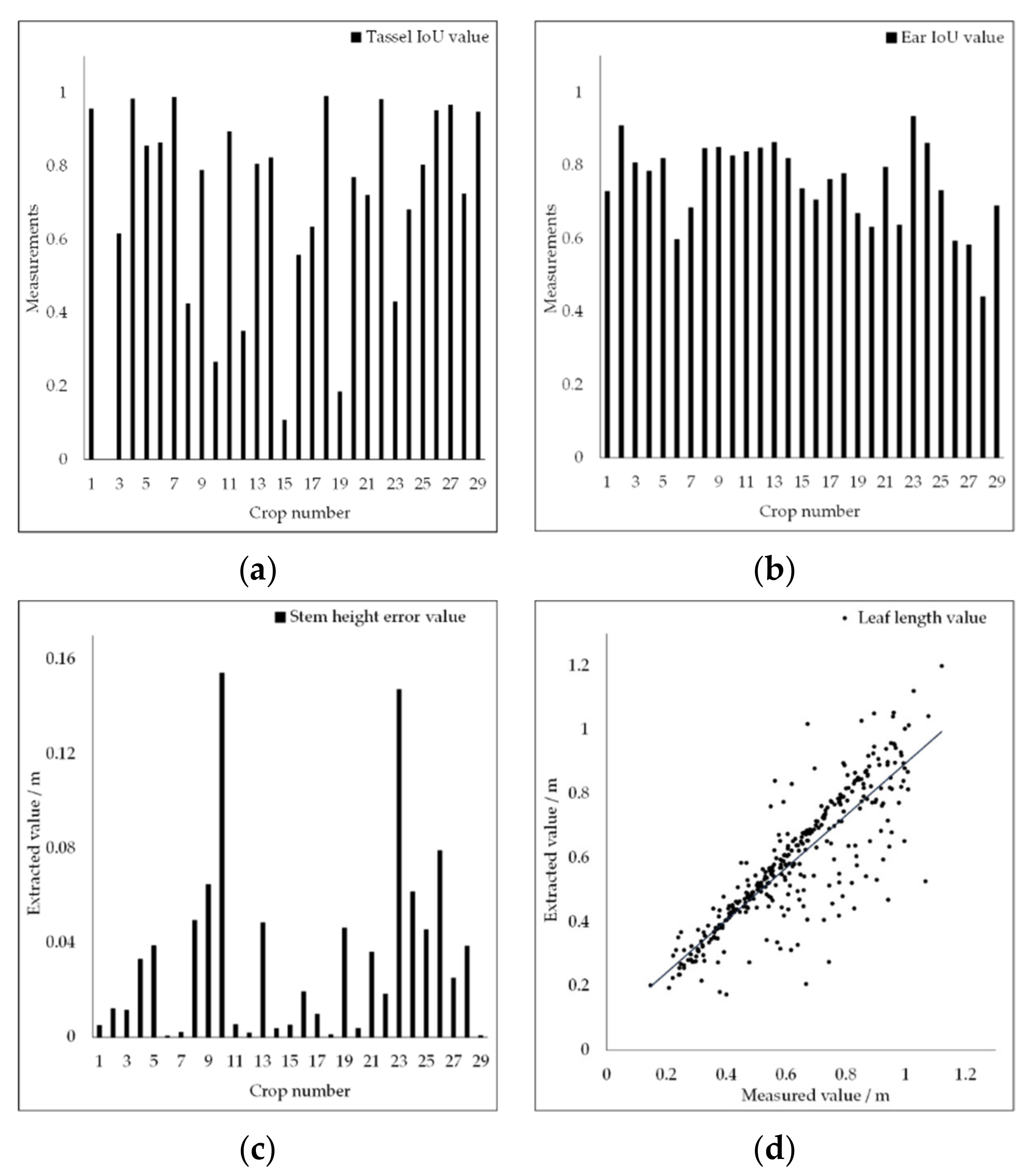
3.2. Organ Stratification Model Accuracy Analysis
4. Conclusions
Author Contributions
Funding
Institutional Review Board Statement
Informed Consent Statement
Data Availability Statement
Conflicts of Interest
References
- Ranum, P.; Peña-Rosas, J.P.; Garcia-Casal, M.N. Global Maize Production, Utilization, and Consumption. Ann. N. Y. Acad. Sci. 2014, 1312, 105–112. [Google Scholar] [CrossRef] [PubMed]
- Indirabai, I.; Nair, M.V.H.; Jaishanker, R.N.; Nidamanuri, R.R. Terrestrial Laser Scanner Based 3D Reconstruction of Trees and Retrieval of Leaf Area Index in a Forest Environment. Ecol. Inform. 2019, 53, 100986. [Google Scholar] [CrossRef]
- Indirabai, I.; Nair, M.V.H.; Nair, J.R.; Nidamanuri, R.R. Direct Estimation of Leaf Area Index of Tropical Forests Using LiDAR Point Cloud. Remote Sens. Appl. Soc. Environ. 2020, 18, 100295. [Google Scholar] [CrossRef]
- Friedli, M.; Kirchgessner, N.; Grieder, C.; Liebisch, F.; Mannale, M.; Walter, A. Terrestrial 3D Laser Scanning to Track the Increase in Canopy Height of Both Monocot and Dicot Crop Species under Field Conditions. Plant Methods 2016, 12, 9. [Google Scholar] [CrossRef]
- Calders, K.; Adams, J.; Armston, J.; Bartholomeus, H.; Bauwens, S.; Bentley, L.P.; Chave, J.; Danson, F.M.; Demol, M.; Disney, M.; et al. Terrestrial Laser Scanning in Forest Ecology: Expanding the Horizon. Remote Sens. Environ. 2020, 251, 112102. [Google Scholar] [CrossRef]
- Barbeito, I.; Dassot, M.; Bayer, D.; Collet, C.; Drössler, L.; Löf, M.; del Rio, M.; Ruiz-Peinado, R.; Forrester, D.I.; Bravo-Oviedo, A.; et al. Terrestrial Laser Scanning Reveals Differences in Crown Structure of Fagus Sylvatica in Mixed vs. Pure European Forests. For. Ecol. Manag. 2017, 405, 381–390. [Google Scholar] [CrossRef]
- De Conto, T.; Olofsson, K.; Görgens, E.B.; Rodriguez, L.C.E.; Almeida, G. Performance of Stem Denoising and Stem Modelling Algorithms on Single Tree Point Clouds from Terrestrial Laser Scanning. Comput. Electron. Agric. 2017, 143, 165–176. [Google Scholar] [CrossRef]
- Hosoi, F.; Nakabayashi, K.; Omasa, K. 3-D Modeling of Tomato Canopies Using a High-Resolution Portable Scanning Lidar for Extracting Structural Information. Sensors 2011, 11, 2166–2174. [Google Scholar] [CrossRef]
- Rosell, J.R.; Sanz, R. A Review of Methods and Applications of the Geometric Characterization of Tree Crops in Agricultural Activities. Comput. Electron. Agric. 2012, 81, 124–141. [Google Scholar] [CrossRef]
- Rose, J.; Paulus, S.; Kuhlmann, H. Accuracy Analysis of a Multi-View Stereo Approach for Phenotyping of Tomato Plants at the Organ Level. Sensors 2015, 15, 9651–9665. [Google Scholar] [CrossRef] [Green Version]
- Li, Y.; Wen, W.; Miao, T.; Wu, S.; Yu, Z.; Wang, X.; Guo, X.; Zhao, C. Automatic Organ-Level Point Cloud Segmentation of Maize Shoots by Integrating High-Throughput Data Acquisition and Deep Learning. Comput. Electron. Agric. 2022, 193, 106702. [Google Scholar] [CrossRef]
- Zhou, J.; Fu, X.; Zhou, S.; Zhou, J.; Ye, H.; Nguyen, H.T. Automated Segmentation of Soybean Plants from 3D Point Cloud Using Machine Learning. Comput. Electron. Agric. 2019, 162, 143–153. [Google Scholar] [CrossRef]
- Paproki, A.; Sirault, X.; Berry, S.; Furbank, R.; Fripp, J. A Novel Mesh Processing Based Technique for 3D Plant Analysis. BMC Plant Biol. 2012, 12, 63. [Google Scholar] [CrossRef]
- Paulus, S.; Dupuis, J.; Mahlein, A.-K.; Kuhlmann, H. Surface Feature Based Classification of Plant Organs from 3D Laserscanned Point Clouds for Plant Phenotyping. BMC Bioinform. 2013, 14, 238. [Google Scholar] [CrossRef]
- Mortensen, A.K.; Bender, A.; Whelan, B.; Barbour, M.M.; Sukkarieh, S.; Karstoft, H.; Gislum, R. Segmentation of Lettuce in Coloured 3D Point Clouds for Fresh Weight Estimation. Comput. Electron. Agric. 2018, 154, 373–381. [Google Scholar] [CrossRef]
- Lin, Y. LiDAR: An Important Tool for next-Generation Phenotyping Technology of High Potential for Plant Phenomics? Comput. Electron. Agric. 2015, 119, 61–73. [Google Scholar] [CrossRef]
- Comba, L.; Biglia, A.; Ricauda Aimonino, D.; Gay, P. Unsupervised Detection of Vineyards by 3D Point-Cloud UAV Photogrammetry for Precision Agriculture. Comput. Electron. Agric. 2018, 155, 84–95. [Google Scholar] [CrossRef]
- White, J.W.; Andrade-Sanchez, P.; Gore, M.A.; Bronson, K.F.; Coffelt, T.A.; Conley, M.M.; Feldmann, K.A.; French, A.N.; Heun, J.T.; Hunsaker, D.J.; et al. Field-Based Phenomics for Plant Genetics Research. Field Crops Res. 2012, 133, 101–112. [Google Scholar] [CrossRef]
- Elnashef, B.; Filin, S.; Lati, R.N. Tensor-Based Classification and Segmentation of Three-Dimensional Point Clouds for Organ-Level Plant Phenotyping and Growth Analysis. Comput. Electron. Agric. 2019, 156, 51–61. [Google Scholar] [CrossRef]
- Miao, T.; Zhu, C.; Xu, T.; Yang, T.; Li, N.; Zhou, Y.; Deng, H. Automatic Stem-Leaf Segmentation of Maize Shoots Using Three-Dimensional Point Cloud. Comput. Electron. Agric. 2021, 187, 106310. [Google Scholar] [CrossRef]
- Wu, G.; Li, B.; Zhu, Q.; Huang, M.; Guo, Y. Using Color and 3D Geometry Features to Segment Fruit Point Cloud and Improve Fruit Recognition Accuracy. Comput. Electron. Agric. 2020, 174, 105475. [Google Scholar] [CrossRef]
- Araus, J.L.; Cairns, J.E. Field High-Throughput Phenotyping: The New Crop Breeding Frontier. Trends Plant Sci. 2014, 19, 52–61. [Google Scholar] [CrossRef]
- Zhou, C.; Yang, G.; Liang, D.; Yang, X.; Xu, B. An Integrated Skeleton Extraction and Pruning Method for Spatial Recognition of Maize Seedlings in MGV and UAV Remote Images. IEEE Trans. Geosci. Remote Sens. 2018, 56, 4618–4632. [Google Scholar] [CrossRef]
- Wu, S.; Wen, W.; Xiao, B.; Guo, X.; Du, J.; Wang, C.; Wang, Y. An Accurate Skeleton Extraction Approach From 3D Point Clouds of Maize Plants. Front. Plant Sci. 2019, 10, 248. [Google Scholar] [CrossRef]
- Jiang, A.; Liu, J.; Zhou, J.; Zhang, M. Skeleton Extraction from Point Clouds of Trees with Complex Branches via Graph Contraction. Vis. Comput. 2021, 37, 2235–2251. [Google Scholar] [CrossRef]
- Cao, W.; Wu, J.; Shi, Y.; Chen, D. Restoration of Individual Tree Missing Point Cloud Based on Local Features of Point Cloud. Remote Sens. 2022, 14, 1346. [Google Scholar] [CrossRef]
- Liu, F.; Song, Q.; Zhao, J.; Mao, L.; Bu, H.; Hu, Y.; Zhu, X. Canopy Occupation Volume as an Indicator of Canopy Photosynthetic Capacity. New Phytol. 2021, 232, 941–956. [Google Scholar] [CrossRef]
- Xiao, F.; Li, W.; Xiao, M.; Yang, Z.; Cheng, W.; Gao, S.; Li, G.; Ding, Y.; Paul, M.J.; Liu, Z. A Novel Light Interception Trait of a Hybrid Rice Ideotype Indicative of Leaf to Panicle Ratio. Field Crops Res. 2021, 274, 108338. [Google Scholar] [CrossRef]
- Qiu, Q.; Sun, N.; Bai, H.; Wang, N.; Fan, Z.; Wang, Y.; Meng, Z.; Li, B.; Cong, Y. Field-Based High-Throughput Phenotyping for Maize Plant Using 3D LiDAR Point Cloud Generated with a “Phenomobile". Front. Plant Sci. 2019, 10, 554. [Google Scholar] [CrossRef]
- Jin, S.; Su, Y.; Wu, F.; Pang, S.; Gao, S.; Hu, T.; Liu, J.; Guo, Q. Stem–Leaf Segmentation and Phenotypic Trait Extraction of Individual Maize Using Terrestrial LiDAR Data. IEEE Trans. Geosci. Remote Sens. 2019, 57, 1336–1346. [Google Scholar] [CrossRef]
- Qi, C.R.; Su, H.; Mo, K.; Guibas, L.J. PointNet: Deep Learning on Point Sets for 3D Classification and Segmentation. In Proceedings of the IEEE Conference on Computer Vision and Pattern Recognition (CVPR), Las Vegas, NV, USA, 27–30 June 2016. [Google Scholar]
- Qi, C.R.; Yi, L.; Su, H.; Guibas, L.J. PointNet++: Deep Hierarchical Feature Learning on Point Sets in a Metric Space. In Proceedings of the Advances in Neural Information Processing Systems 30: Annual Conference on Neural Information Processing Systems 2017, Long Beach, CA, USA, 4–9 December 2017. [Google Scholar]
- Li, T.; Feng, Q.; Qiu, Q.; Xie, F.; Zhao, C. Occluded Apple Fruit Detection and Localization with a Frustum-Based Point-Cloud-Processing Approach for Robotic Harvesting. Remote Sens. 2022, 14, 482. [Google Scholar] [CrossRef]
- Schmohl, S.; Narváez Vallejo, A.; Soergel, U. Individual Tree Detection in Urban ALS Point Clouds with 3D Convolutional Networks. Remote Sens. 2022, 14, 1317. [Google Scholar] [CrossRef]
- Jin, S.; Su, Y.; Gao, S.; Wu, F.; Hu, T.; Liu, J.; Li, W.; Wang, D.; Chen, S.; Jiang, Y.; et al. Deep Learning: Individual Maize Segmentation From Terrestrial Lidar Data Using Faster R-CNN and Regional Growth Algorithms. Front. Plant Sci. 2018, 9, 866. [Google Scholar] [CrossRef] [PubMed]
- Deery, D.; Jimenez-Berni, J.; Jones, H.; Sirault, X.; Furbank, R. Proximal Remote Sensing Buggies and Potential Applications for Field-Based Phenotyping. Agronomy 2014, 4, 349–379. [Google Scholar] [CrossRef]
- Magney, T.S.; Eusden, S.A.; Eitel, J.U.H.; Logan, B.A.; Jiang, J.; Vierling, L.A. Assessing Leaf Photoprotective Mechanisms Using Terrestrial LiDAR: Towards Mapping Canopy Photosynthetic Performance in Three Dimensions. New Phytol. 2014, 201, 344–356. [Google Scholar] [CrossRef] [PubMed]
- Eitel, J.U.H.; Magney, T.S.; Vierling, L.A.; Brown, T.T.; Huggins, D.R. LiDAR Based Biomass and Crop Nitrogen Estimates for Rapid, Non-Destructive Assessment of Wheat Nitrogen Status. Field Crops Res. 2014, 159, 21–32. [Google Scholar] [CrossRef]
- Kjaer, K.; Ottosen, C.-O. 3D Laser Triangulation for Plant Phenotyping in Challenging Environments. Sensors 2015, 15, 13533–13547. [Google Scholar] [CrossRef]
- Deng, X.; Tang, G.; Wang, Q. A Novel Fast Classification Filtering Algorithm for LiDAR Point Clouds Based on Small Grid Density Clustering. Geod. Geodyn. 2022, 13, 38–49. [Google Scholar] [CrossRef]
- Czerniawski, T.; Sankaran, B.; Nahangi, M.; Haas, C.; Leite, F. 6D DBSCAN-Based Segmentation of Building Point Clouds for Planar Object Classification. Autom. Constr. 2018, 88, 44–58. [Google Scholar] [CrossRef]
- Ferrara, R.; Virdis, S.G.P.; Ventura, A.; Ghisu, T.; Duce, P.; Pellizzaro, G. An Automated Approach for Wood-Leaf Separation from Terrestrial LIDAR Point Clouds Using the Density Based Clustering Algorithm DBSCAN. Agric. For. Meteorol. 2018, 262, 434–444. [Google Scholar] [CrossRef]
- Sugiyama, M. Clustering. In Introduction to Statistical Machine Learning; Elsevier: Amsterdam, The Netherlands, 2016; Volume 37, pp. 447–456. [Google Scholar]
- Ester, M.; Kriegel, H.-P.; Sander, J.; Xu, X. A Density-Based Algorithm for Discovering Clusters in Large Spatial Databases with Noise. In KDD-96 Proceedings; Simoudis, E., Ed.; AAAI Press: Palo Alto, CA, USA, 1996. [Google Scholar]
- Wald, I.; Havran, V. On Building Fast Kd-Trees for Ray Tracing, and on Doing That in O(N Log N). In Proceedings of the 2006 IEEE Symposium on Interactive Ray Tracing, Salt Lake City, UT, USA, 18–20 September 2006; pp. 61–69. [Google Scholar]
- Shi, J.; Malik, J. Normalized Cuts and Image Segmentation. IEEE Trans. Pattern Anal. Mach. Intell. 2000, 22, 888–905. [Google Scholar] [CrossRef] [Green Version]


| Number | Type of Maize | Acquisition Date (Day/Month/Year) | Maize Numbers | Growing Stage | Area Size | Number of Scan Stations | Number of Scan Points | Average Position Deviation |
|---|---|---|---|---|---|---|---|---|
| Maize-01 | Feed grade yellow maize | 13 July 2021 | 89 | Seedling stage | 5.9 × 3.4 m | 8 | 12,585,028 | 0.61 mm |
| Maize-02 | Sweet maize | 17 July 2021 | 89 | heading stage | 6.1 × 3.9 m | 8 | 11,686,560 | 0.64 mm |
| Maize-03 | Sweet maize | 29 July 2021 | 90 | heading stage | 5.9 × 3.6 m | 8 | 10,688,590 | 0.73 mm |
| Maize-04 | Waxy maize | 30 July 2021 | 29 | Full ripening stage | 4.0 × 2.7 m | 8 | 12,920,643 | 0.69 mm |
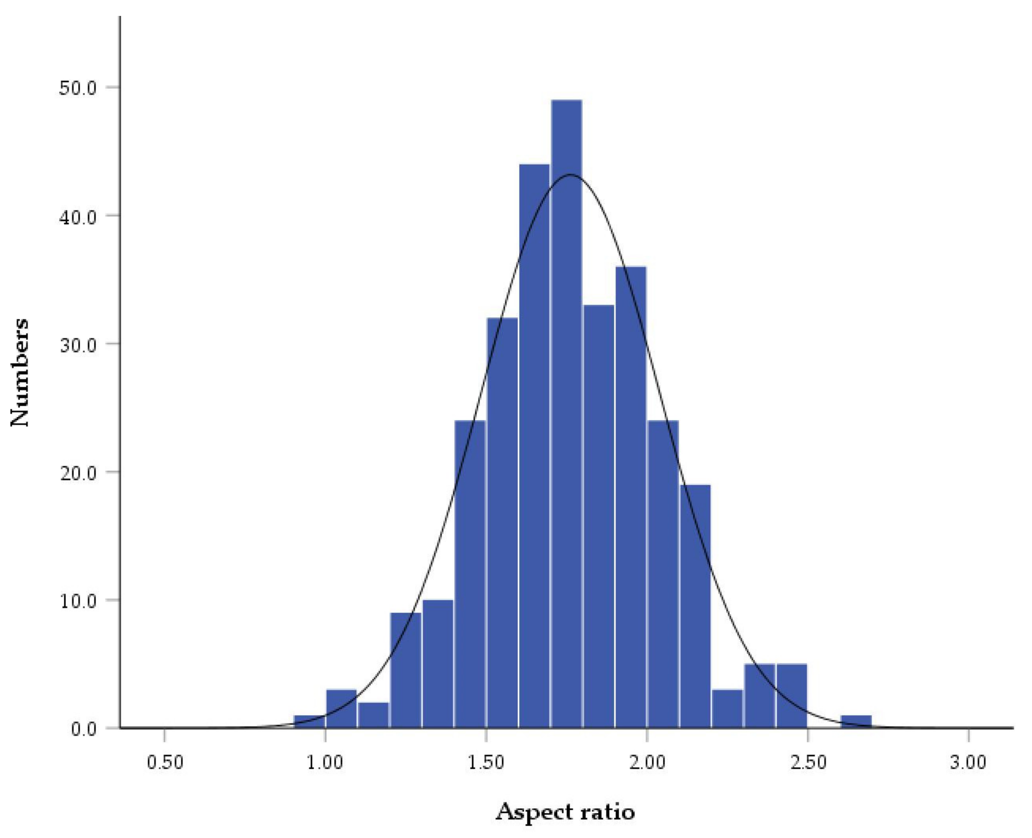
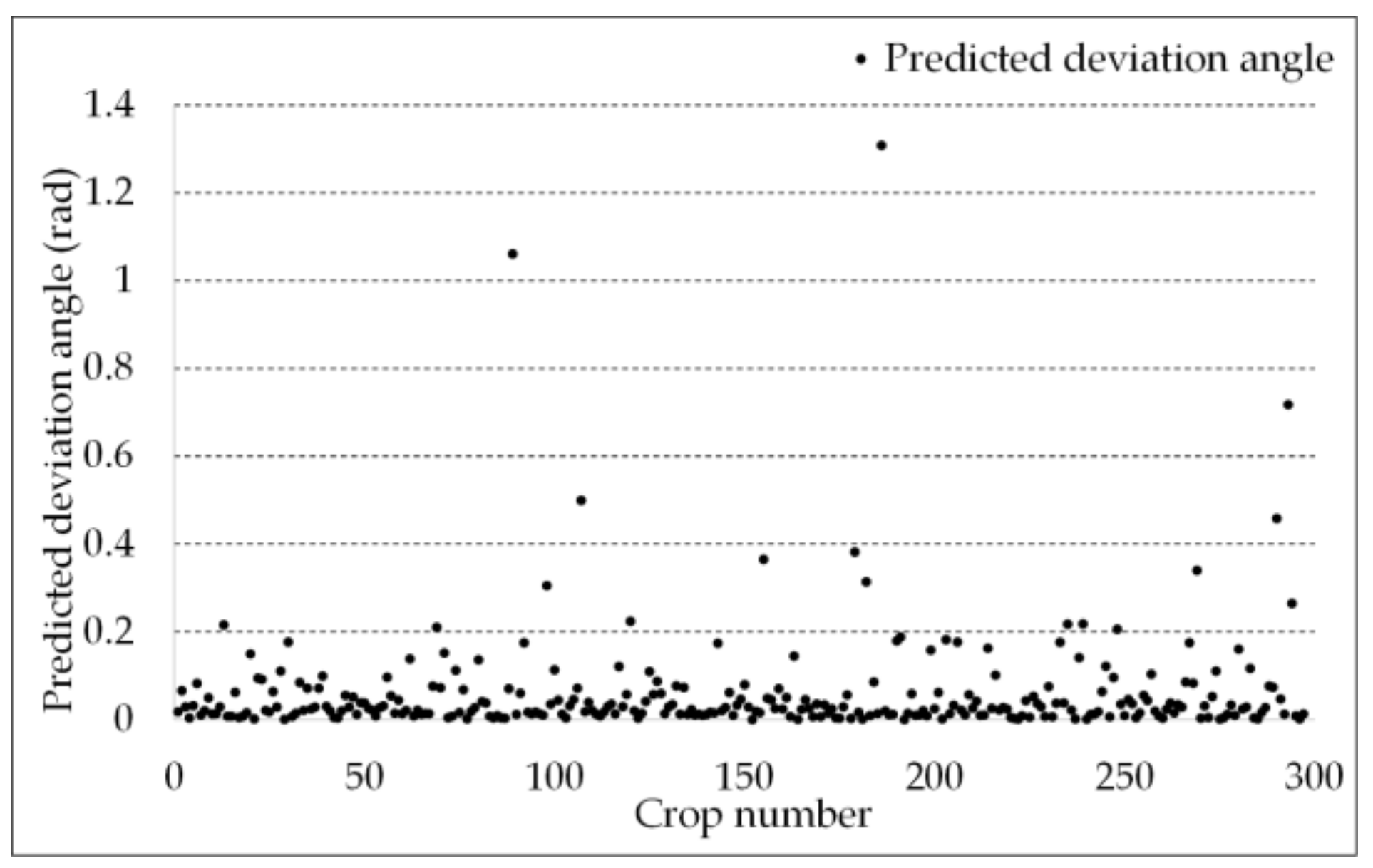
| N | Skewness | Kurtosis | |||
|---|---|---|---|---|---|
| Statistic | Std. Error | Statistic | Std. Error | ||
| Valid N | 300 | 0.113 | 0.141 | 0.161 | 0.281 |
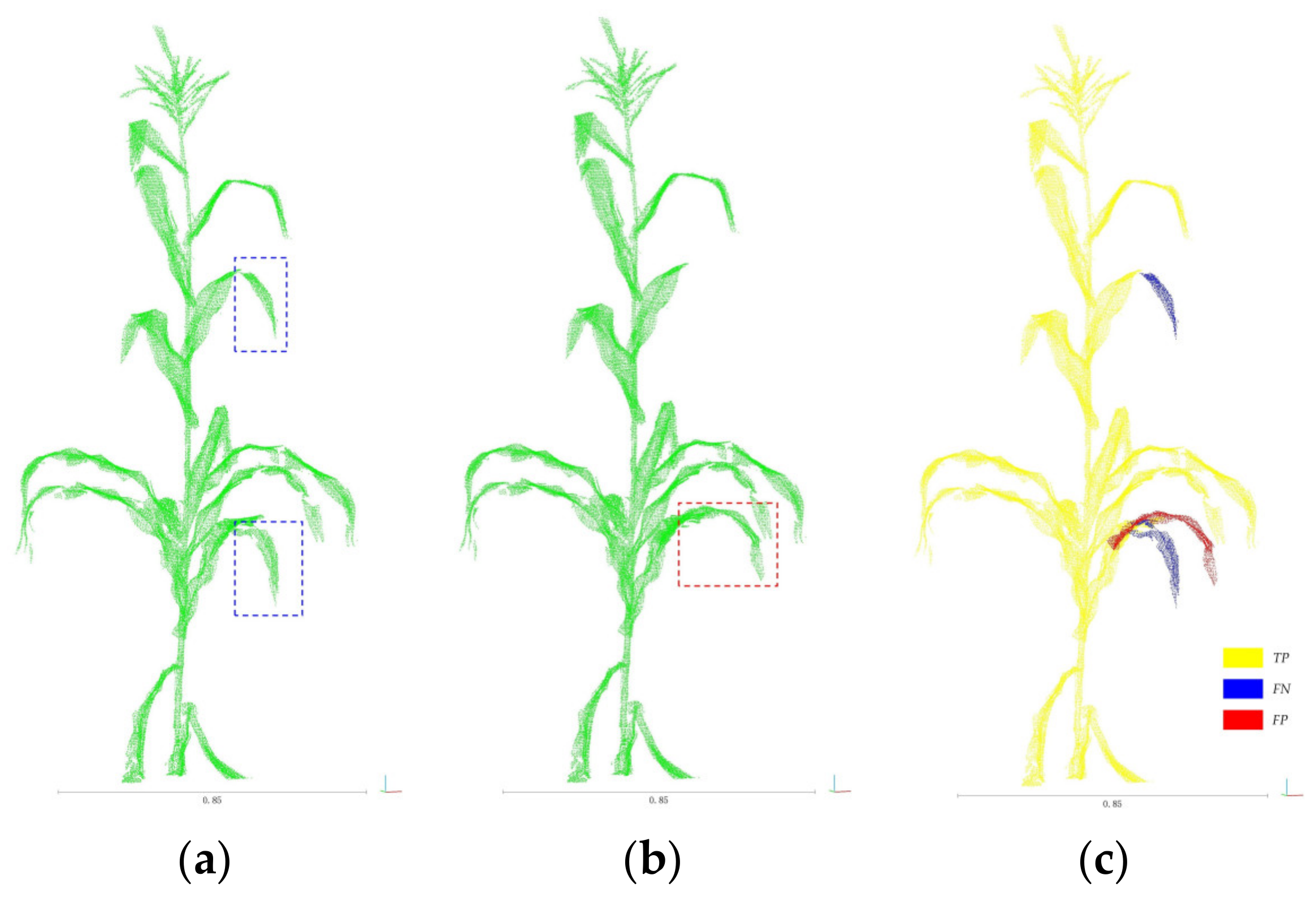
| TP (Yellow) | FN (Blue) | FP (Red) | P | R | F-Score | OA | |||||||
|---|---|---|---|---|---|---|---|---|---|---|---|---|---|
| [0, 80%] | [80%, 95%] | [95%, 100%] | [0, 80%] | [80%, 95%] | [95%, 100%] | [0, 80%] | [80%, 95%] | [95%, 100%] | |||||
| Maize-01 | 5,727,642 | 73,579 | 62,781 | 0 | 13 | 76 | 3 | 22 | 64 | 0 | 28 | 61 | 0.98 |
| Maize-02 | 8,826,515 | 157,479 | 108,064 | 3 | 16 | 70 | 1 | 23 | 65 | 0 | 27 | 62 | 0.97 |
| Maize-03 | 9,815,061 | 268,093 | 285,177 | 4 | 20 | 66 | 3 | 15 | 72 | 1 | 23 | 66 | 0.95 |
| Maize-04 | 5,913,240 | 228,412 | 123,822 | 1 | 2 | 26 | 0 | 11 | 18 | 0 | 6 | 23 | 0.94 |
Publisher’s Note: MDPI stays neutral with regard to jurisdictional claims in published maps and institutional affiliations. |
© 2022 by the authors. Licensee MDPI, Basel, Switzerland. This article is an open access article distributed under the terms and conditions of the Creative Commons Attribution (CC BY) license (https://creativecommons.org/licenses/by/4.0/).
Share and Cite
Lin, C.; Hu, F.; Peng, J.; Wang, J.; Zhai, R. Segmentation and Stratification Methods of Field Maize Terrestrial LiDAR Point Cloud. Agriculture 2022, 12, 1450. https://doi.org/10.3390/agriculture12091450
Lin C, Hu F, Peng J, Wang J, Zhai R. Segmentation and Stratification Methods of Field Maize Terrestrial LiDAR Point Cloud. Agriculture. 2022; 12(9):1450. https://doi.org/10.3390/agriculture12091450
Chicago/Turabian StyleLin, Chengda, Fangzheng Hu, Junwen Peng, Jing Wang, and Ruifang Zhai. 2022. "Segmentation and Stratification Methods of Field Maize Terrestrial LiDAR Point Cloud" Agriculture 12, no. 9: 1450. https://doi.org/10.3390/agriculture12091450
APA StyleLin, C., Hu, F., Peng, J., Wang, J., & Zhai, R. (2022). Segmentation and Stratification Methods of Field Maize Terrestrial LiDAR Point Cloud. Agriculture, 12(9), 1450. https://doi.org/10.3390/agriculture12091450