


An Empirical Investigation into Greenhouse Gas Emissions and Agricultural Economic Performance in Baltic Countries: A Non-Linear Framework

 , and
, and
Abstract
:1. Introduction
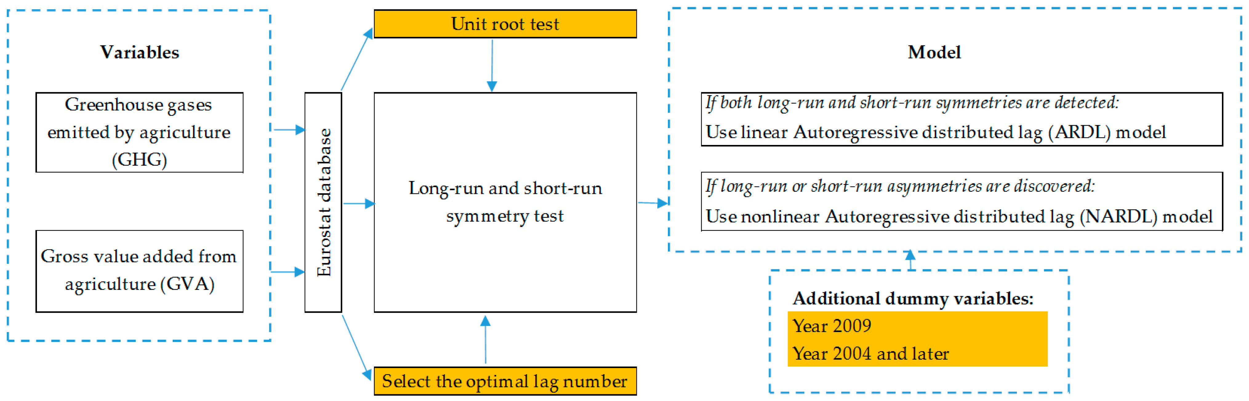
2. Materials and Methods
2.1. Methods
2.2. Data Sources
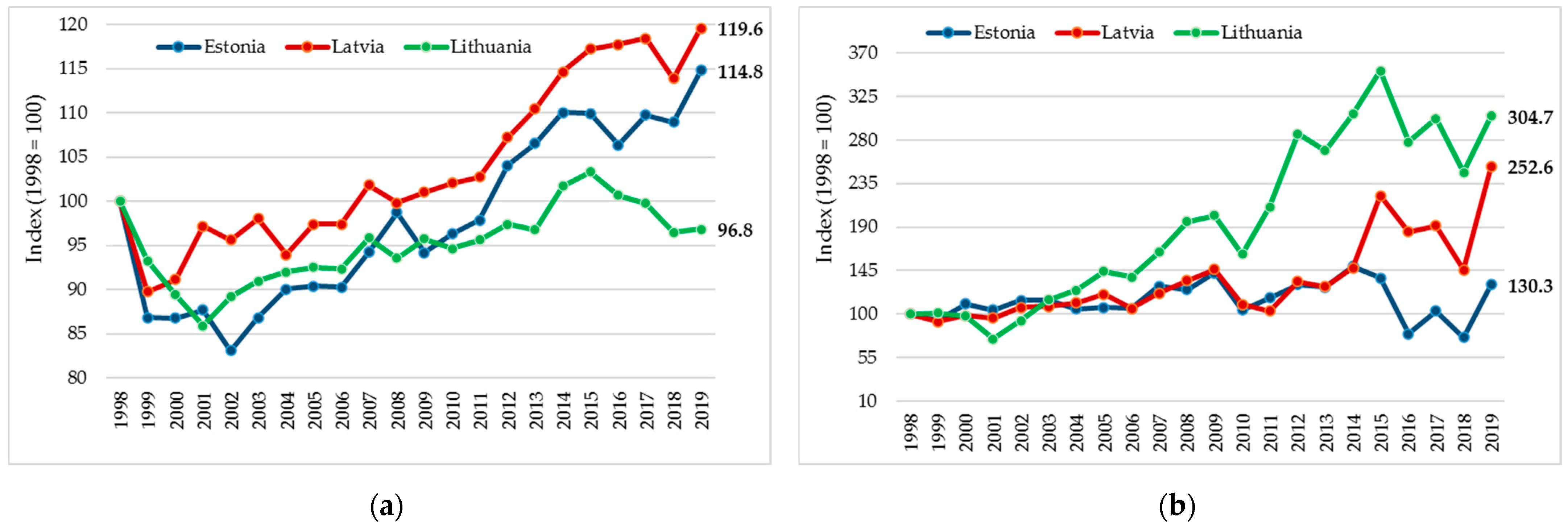
3. Results
4. Discussion
4.1. Contextualization with Previous Research
4.2. Future Research Guidelines
4.3. Practical Implications
5. Conclusions
Author Contributions
Funding
Institutional Review Board Statement
Informed Consent Statement
Data Availability Statement
Conflicts of Interest
Appendix A

| Information Criteria | Schwarz Criterion | Akaike Criterion | Hannan-QUINN Criterion | ||||||
|---|---|---|---|---|---|---|---|---|---|
| Time Lag | q = 1 | q = 2 | q = 3 | q = 1 | q = 2 | q = 3 | q = 1 | q = 2 | q = 3 |
| Lithuania | |||||||||
| p = 1 | 238.1 | 233.4 | 228.3 | 231.1 | 224.4 | 217.9 | 232.5 | 226.2 | 219.6 |
| p = 2 | 225.7 | 213.4 | 209.3 | 218.1 | 204.0 | 198.0 | 219.4 | 205.6 | 199.9 |
| Latvia | |||||||||
| p = 1 | 226.2 | 229.0 | 215.6 | 219.2 | 220.0 | 205.3 | 220.6 | 221.8 | 207.0 |
| p = 2 | 219.0 | 221.1 | 217.9 | 211.4 | 211.6 | 206.5 | 212.7 | 213.2 | 208.5 |
| Estonia | |||||||||
| p = 1 | 207.6 | 213.4 | 194.9 | 200.7 | 204.5 | 184.5 | 202.0 | 206.2 | 186.3 |
| p = 2 | 201.3 | 207.2 | 195.5 | 193.7 | 197.7 | 184.1 | 195.0 | 199.3 | 186.1 |
| Panel | |||||||||
| p = 1 | 686.4 | 694.5 | 652.9 | 671.8 | 675.7 | 630.5 | 677.5 | 683.0 | 639.2 |
| p = 2 | 648.4 | 654.5 | 656.7 | 632.1 | 634.1 | 632.2 | 638.4 | 642.0 | 641.7 |
Appendix B
| Variable | Coefficient | p-Value |
|---|---|---|
| Constant | 7007.23 | <0.0001 |
| GHG (−1) | −1.7567 | <0.0001 |
| GVA+ (−1) | 0.6828 | <0.0001 |
| GVA– (−1) | 0.9376 | 0.0001 |
| ΔGHG (−1) | 0.5356 | 0.0048 |
| ΔGHG (−2) | 0.4279 | 0.0022 |
| ΔGVA (0) | 0.2385 | 0.0002 |
| ΔGVA (−1) | −0.4303 | 0.0010 |
| ΔGVA (−2) | −0.1924 | 0.0192 |
| Additional hypotheses: h1: reject, p-value 0.0002 h2: reject, p-value < 0.0001 h3: reject, p-value < 0.0001 Long-run coefficients: , p-value: 0.8390 , p-value: 0.7414 | Additional estimations, p-values: Normality of residual: 0.0016 Unit-root of residual (constant): 0.1893 Unit-root of residual (trend): 0.6138 ARCH effect: 0.9308 R-squared: 0.9224 QLR test p-value: 0.0216, year: 2011 | |
Appendix C
| Variable | Coefficient | p-Value |
|---|---|---|
| Constant | 21.29 | 0.0875 |
| ΔGVA (0) | 0.2275 | 0.0300 |
| Additional estimations, p-values: Normality of residual: 0.7553 Unit-root of residual (constant): 0.0110 Unit-root of residual (trend): 0.6849 ARCH effect: 0.6540 R-squared: 0.2480 QLR test p-value: 0.1716, year: 2002 | ||
Appendix D
| Variable | Coefficient | p-Value |
|---|---|---|
| Constant | 789.94 | 0.0016 |
| GHG (−1) | −0.7515 | 0.0015 |
| GVA+ (−1) | 0.9025 | 0.0016 |
| GVA– (−1) | 0.3309 | 0.0166 |
| ΔGVA (0) | 0.4034 | 0.0005 |
| S_2004 | 44.0169 | 0.0229 |
| D_2009 | −77.2390 | 0.0110 |
| Additional hypotheses: h1: reject, p-value 0.0082 Long-run coefficients: , p-value: 0.2127 , p-value: 0.4303 | Additional estimations, p-values: Normality of residual: 0.3051 Unit-root of residual (constant): 0.0110 Unit-root of residual (trend): 0.6849 ARCH effect: 0.1004 R-squared: 0.8174 | |
References
- European Environment Agency. Climate Change Mitigation. Available online: https://www.eea.europa.eu/themes/climate/intro (accessed on 15 December 2021).
- IPCC Summary for Policymakers Climate Change 2022: Impacts, Adaptation and Vulnerability. Part B: Observed and Projected Impacts and Risks; Pörtner, H.-O.; Roberts, M.; Tignor, E.S.; Poloczanska, K.; Mintenbeck, A.; Alegría, M.; Craig, S.; Langsdorf, S.; Löschke, V.; Möller, A.; et al. (Eds.) Cambridge University Press: Cambridge, UK, 2022. [Google Scholar]
- Zafeiriou, E.; Sofios, S.; Partalidou, X. Environmental Kuznets curve for EU agriculture: Empirical evidence from new entrant EU countries. Environ. Sci. Pollut. Res. 2017, 24, 15510–15520. [Google Scholar] [CrossRef] [PubMed]
- European Environment Agency. Agriculture and Climate Change. Available online: https://www.eea.europa.eu/media/infographics/climate-change-and-agriculture/view (accessed on 5 December 2021).
- Li, T.; Baležentis, T.; Makutėnienė, D.; Streimikiene, D.; Kriščiukaitienė, I. Energy-related CO2 emission in European Union agriculture: Driving forces and possibilities for reduction. Appl. Energy 2016, 180, 682–694. [Google Scholar] [CrossRef]
- Yan, Q.; Yin, J.; Baležentis, T.; Makutėnienė, D.; Štreimikienė, D. Energy-related GHG emission in agriculture of the European countries: An application of the Generalized Divisia Index. J. Clean. Prod. 2017, 164, 686–694. [Google Scholar] [CrossRef]
- Garnier, J.; Le Noë, J.; Marescaux, A.; Sanz-Cobena, A.; Lassaletta, L.; Silvestre, M.; Thieu, V.; Billen, G. Long-term changes in greenhouse gas emissions from French agriculture and livestock (1852–2014): From traditional agriculture to conventional intensive systems. Sci. Total Environ. 2019, 660, 1486–1501. [Google Scholar] [CrossRef] [PubMed]
- Mohammed, S.; Alsafadi, K.; Takács, I.; Harsányi, E. Contemporary changes of greenhouse gases emission from the agricultural sector in the EU-27. Geol. Ecol. Landsc. 2020, 4, 282–287. [Google Scholar] [CrossRef]
- Eurostat; European Commission. Greenhouse Gas Emissions by Source Sector (Source: EEA). Eurostat. Available online: https://appsso.eurostat.ec.europa.eu/nui/show.do?dataset=env_air_gge&lang=en (accessed on 11 April 2022).
- IPCC Summary for Policymakers Climate Change 2014: Impacts, Adaptation and Vulnerability. Part A: Global and Sectoral Aspects; Field, C.B.; Barros, V.R.; Dokken, D.J.; Mach, K.J.; Mastrandrea, M.D.; Bilir, T.E.; Chatterjee, M.C.; Ebi, K.L.; Estrada, Y.O.; Genova, R.C.; et al. (Eds.) Cambridge University Press: Cambridge, UK, 2014. [Google Scholar]
- Karimi, V.; Karami, E.; Keshavarz, M. Climate change and agriculture: Impacts and adaptive responses in Iran. J. Integr. Agric. 2018, 17, 1–15. [Google Scholar] [CrossRef]
- Kar, A.K. Environmental Kuznets curve for CO2 emissions in Baltic countries: An empirical investigation. Environ. Sci. Pollut. Res. 2022, 29, 47189–47208. [Google Scholar] [CrossRef]
- Communication from the Commission. The European Green Deal. Brussels, 11 December 2019. COM(2019) 640 Final. Available online: https://eur-lex.europa.eu/legal-content/EN/TXT/?qid=1576150542719&uri=COM%3A2019%3A640%3AFIN (accessed on 8 December 2021).
- Communication from the Commission. A Farm to Fork Strategy for a Fair, Healthy and Environmentally-Friendly Food System. Brussels, 20 May 2020. COM(2020) 381 Final. Available online: https://eur-lex.europa.eu/legal-content/EN/TXT/?uri=CELEX:52020DC0381 (accessed on 10 December 2021).
- Communication from the Commission. EU Biodiversity Strategy for 2030. Brussels, 20 May 2020 COM(2020) 380 Final. Available online: https://eur-lex.europa.eu/legal-content/EN/TXT/?qid=1590574123338&uri=CELEX:52020DC0380 (accessed on 9 December 2021).
- Communication from the Commission to the European Parliament, the Council, the European Economic and Social Committee of the Regions a New Circular Economy Action Plan for a Cleaner and More Competitive Europe. COM/2020/98 Final. Available online: https://eur-lex.europa.eu/legal-content/EN/TXT/?qid=1583933814386&uri=COM:2020:98:FIN (accessed on 8 December 2021).
- Grossman, G.M.; Krueger, A.B. Environmental Impacts of a North American Free Trade Agreement; Working Paper No. 3914; National Bureau of Economic Research: Cambridge, MA, USA, 1991. [Google Scholar]
- Beckerman, W. Economic growth and the environment: Whose growth? Whose environment? World Dev. 1992, 20, 481–496. [Google Scholar] [CrossRef]
- Panayotou, T. Empirical Tests and Policy Analysis of Environmental Degradation at Different Stages of Economic Development (No. 992927783402676); International Labour Organization: Geneva, Switzerland, 1993. [Google Scholar]
- Grossman, G.M.; Krueger, A.B. Economic growth and the environment. Q. J. Econ. 1995, 110, 353–377. [Google Scholar] [CrossRef]
- Gill, A.R.; Viswanathan, K.K.; Hassan, S. The Environmental Kuznets Curve (EKC) and the environmental problem of the day. Renew. Sustain. Energy Rev. 2018, 81, 1636–1642. [Google Scholar] [CrossRef]
- Kaika, D.; Zervas, E. The Environmental Kuznets Curve (EKC) theory—Part A: Concept, causes and the CO2 emissions case. Energy Policy 2013, 62, 1392–1402. [Google Scholar] [CrossRef]
- Chen, Q.; Taylor, D. Economic development and pollution emissions in Singapore: Evidence in support of the Environmental Kuznets Curve hypothesis and its implications for regional sustainability. J. Clean. Prod. 2020, 243, 118637. [Google Scholar] [CrossRef]
- Destek, M.A.; Sarkodie, S.A. Investigation of environmental Kuznets curve for ecological footprint: The role of energy and financial development. Sci. Total Environ. 2019, 650, 2483–2489. [Google Scholar] [CrossRef]
- Balibey, M. Relationships among CO2 emissions, economic growth and foreign direct investment and the environmental Kuznets curve hypothesis in Turkey. Int. J. Energy Econ. Policy 2015, 5, 1042–1049. [Google Scholar]
- Sarkodie, S.A.; Strezov, V. Empirical study of the environmental Kuznets curve and environmental sustainability curve hypothesis for Australia, China, Ghana and USA. J. Clean. Prod. 2018, 201, 98–110. [Google Scholar] [CrossRef]
- Bekhet, H.A.; Othman, N.S. The role of renewable energy to validate dynamic interaction between CO2 emissions and GDP toward sustainable development in Malaysia. Energy Econ. 2018, 72, 47–61. [Google Scholar] [CrossRef]
- Zambrano-Monserrate, M.A.; Silva-Zambrano, C.A.; Davalos-Penafiel, J.L.; Zambrano-Monserrate, A.; Ruano, M.A. Testing environmental Kuznets curve hypothesis in Peru: The role of renewable electricity, petroleum and dry natural gas. Renew. Sustain. Energy Rev. 2018, 82, 4170–4178. [Google Scholar] [CrossRef]
- Sinha, A.; Shahbaz, M. Estimation of environmental Kuznets curve for CO2 emission: Role of renewable energy generation in India. Renew. Energy 2018, 119, 703–711. [Google Scholar] [CrossRef]
- Dong, K.; Sun, R.; Jiang, H.; Zeng, X. CO2 emissions, economic growth, and the environmental Kuznets curve in China: What roles can nuclear energy and renewable energy play? J. Clean. Prod. 2018, 196, 51–63. [Google Scholar] [CrossRef]
- Balado-Naves, R.; Baños-Pino, J.F.; Mayor, M. Do countries influence neighbouring pollution? A spatial analysis of the EKC for CO2 emissions. Energy Policy 2018, 123, 266–279. [Google Scholar] [CrossRef]
- Xie, Q.; Xu, X.; Liu, X. Is there an EKC between economic growth and smog pollution in China? New evidence from semiparametric spatial autoregressive models. J. Clean. Prod. 2019, 220, 873–883. [Google Scholar] [CrossRef]
- Balsalobre-Lorente, D.; Shahbaz, M.; ChiappettaJabbour, C.J.; Driha, O.M. The role of energy innovation and corruption in carbon emissions: Evidence based on the EKC hypothesis. In Energy and Environmental Strategies in the Era of Globalization; Springer: Cham, Switzerland, 2019; pp. 271–304. [Google Scholar]
- Baležentis, T.; Streimikiene, D.; Zhang, T.; Liobikiene, G. The role of bioenergy in greenhouse gas emission reduction in EU countries: An Environmental Kuznets Curve modelling. Resour. Conserv. Recycl. 2019, 142, 225–231. [Google Scholar] [CrossRef]
- Chen, Y.; Wang, Z.; Zhong, Z. CO2 emissions, economic growth, renewable and non-renewable energy production and foreign trade in China. Renew. Energy 2019, 131, 208–216. [Google Scholar] [CrossRef]
- Shahbaz, M. Globalization–emissions nexus: Testing the EKC hypothesis in Next-11 Countries. Glob. Bus. Rev. 2022, 23, 75–100. [Google Scholar] [CrossRef]
- Erdogan, S.; Adedoyin, F.F.; Bekun, F.V.; Sarkodie, S.A. Testing the transport-induced environmental Kuznets curve hypothesis: The role of air and railway transport. J. Air Transp. Manag. 2020, 89, 101935. [Google Scholar] [CrossRef]
- Ongan, S.; Isik, C.; Ozdemir, D. Economic growth and environmental degradation: Evidence from the US case environmental Kuznets curve hypothesis with application of decomposition. J. Environ. Econ. Policy 2021, 10, 14–21. [Google Scholar] [CrossRef]
- Shah, S.A.R.; Naqvi, S.A.A.; Nasreen, S.; Abbas, N. Associating drivers of economic development with environmental degradation: Fresh evidence from Western Asia and North African region. Ecol. Indic. 2021, 126, 107638. [Google Scholar] [CrossRef]
- Tiwari, A.K.; Shahbaz, M.; Hye, Q.M.A. The environmental Kuznets curve and the role of coal consumption in India: Cointegration and causality analysis in an open economy. Renew. Sustain. Energy Rev. 2013, 18, 519–527. [Google Scholar] [CrossRef]
- Tan, F.; Lean, H.H.; Khan, H. Growth and environmental quality in Singapore: Is there any trade-off? Ecol. Indic. 2014, 47, 149–155. [Google Scholar] [CrossRef]
- Saidi, K.; Mbarek, M.B. The impact of income, trade, urbanization, and financial development on CO2 emissions in 19 emerging economies. Environ. Sci. Pollut. Res. 2017, 24, 12748–12757. [Google Scholar] [CrossRef]
- Pata, U.K. Renewable energy consumption, urbanization, financial development, income and CO2 emissions in Turkey: Testing EKC hypothesis with structural breaks. J. Clean. Prod. 2018, 187, 770–779. [Google Scholar] [CrossRef]
- Zoundi, Z. CO2 emissions, renewable energy and the Environmental Kuznets Curve, a panel cointegration approach. Renew. Sustain. Energy Rev. 2017, 72, 1067–1075. [Google Scholar] [CrossRef]
- Apergis, N.; Ozturk, I. Testing environmental Kuznets curve hypothesis in Asian countries. Ecol. Indic. 2015, 52, 16–22. [Google Scholar] [CrossRef]
- Osabuohien, E.S.; Efobi, U.R.; Gitau, C.M.W. Beyond the environmental Kuznets curve in Africa: Evidence from panel cointegration. J. Environ. Policy Plan. 2014, 16, 517–538. [Google Scholar] [CrossRef]
- Liu, X.; Zhang, S.; Bae, J. The impact of renewable energy and agriculture on carbon dioxide emissions: Investigating the environmental Kuznets curve in four selected ASEAN countries. J. Clean. Prod. 2017, 164, 1239–1247. [Google Scholar] [CrossRef]
- Rupasingha, A.; Goetz, S.J.; Debertin, D.L.; Pagoulatos, A. The environmental Kuznets curve for US counties: A spatial econometric analysis with extensions. Pap. Reg. Sci. 2004, 83, 407–424. [Google Scholar] [CrossRef]
- Lau, L.S.; Choong, C.K.; Eng, Y.K. Investigation of the environmental Kuznets curve for carbon emissions in Malaysia: Do foreign direct investment and trade matter? Energy Policy 2014, 68, 490–497. [Google Scholar] [CrossRef]
- Dinda, S. Environmental Kuznets curve hypothesis: A survey. Ecol. Econ. 2004, 49, 431–455. [Google Scholar] [CrossRef]
- Mert, M.E.R.T.; Bölük, G.; Büyükyilmaz, A. Fossil & renewable energy consumption, GHGs and economic growth: Evidence from a ridge regression of Kyoto annex countries. Akdeniz İİbf Derg. 2015, 15, 45–69. [Google Scholar]
- Pata, U.K.; Aydin, M. Testing the EKC hypothesis for the top six hydropower energy-consuming countries: Evidence from Fourier Bootstrap ARDL procedure. J. Clean. Prod. 2020, 264, 121699. [Google Scholar] [CrossRef]
- Ben Jebli, M.; Ben Youssef, S.; Ozturk, I. The Environmental Kuznets Curve: The Role of Renewable and Non-Renew Energy Consumption and Trade Openness; Munich Personal RePEc Archive: Munich, Germany, 2013. [Google Scholar]
- Robalino-López, A.; Mena-Nieto, Á.; García-Ramos, J.E.; Golpe, A.A. Studying the relationship between economic growth, CO2 emissions, and the environmental Kuznets curve in Venezuela (1980–2025). Renew. Sustain. Energy Rev. 2015, 41, 602–614. [Google Scholar] [CrossRef]
- Chiu, Y.B. Deforestation and the environmental Kuznets curve in developing countries: A panel smooth transition regression approach. Can. J. Agric. Econ. /Rev. Can. 2012, 60, 177–194. [Google Scholar] [CrossRef]
- Alonzo, R.P.; Puzon, K.M. Environmental quality, economic development, and political institutions in East Asia: A survey of issues. DLSU Bus. Econ. Rev. 2013, 22, 15–36. [Google Scholar]
- Farhani, S.; Mrizak, S.; Chaibi, A.; Rault, C. The environmental Kuznets curve and sustainability: A panel data analysis. Energy Policy 2014, 71, 189–198. [Google Scholar] [CrossRef]
- Alvarado, R.; Toledo, E. Environmental degradation and economic growth: Evidence for a developing country. Environ. Dev. Sustain. 2017, 19, 1205–1218. [Google Scholar] [CrossRef]
- Zafeiriou, E.; Mallidis, I.; Galanopoulos, K.; Arabatzis, G. Greenhouse gas emissions and economic performance in EU agriculture: An empirical study in a non-linear framework. Sustainability 2018, 10, 3837. [Google Scholar] [CrossRef]
- Asumadu-Sarkodie, S.; Owusu, P.A. The relationship between carbon dioxide and agriculture in Ghana: A comparison of VECM and ARDL model. Environ. Sci. Pollut. Res. 2016, 23, 10968–10982. [Google Scholar] [CrossRef]
- Pesaran, M.H.; Shin, Y.; Smith, R.J. Bounds testing approaches to the analysis of level relationships. J. Appl. Econom. 2001, 16, 289–326. [Google Scholar] [CrossRef]
- Shin, Y.; Yu, B.; Greenwood-Nimmo, M. Modelling asymmetric cointegration and dynamic multipliers in a nonlinear ARDL framework. In Festschrift in Honor of Peter Schmidt; Springer: New York, NY, USA, 2014; pp. 281–314. [Google Scholar]
- Wald, A. Tests of statistical hypotheses concerning several parameters when the number of observations is large. Trans. Am. Math. Soc. 1943, 54, 426–482. [Google Scholar] [CrossRef]
- Ditzen, J. Estimating Long Run Effects in Models with Cross-Sectional Dependence Using xtdcce2; Working Paper; Centre for Energy Economics Research and Policy: Edinburgh, UK, 2019. [Google Scholar]
- Blackburne, E.F.; Frank, M.W. Estimation of nonstationary heterogeneous panels. Stata J. 2007, 7, 197–208. [Google Scholar] [CrossRef]
- Quandt, R.E. Tests of the hypothesis that a linear regression system obeys two separate regimes. J. Am. Stat. Assoc. 1960, 55, 324–330. [Google Scholar] [CrossRef]
- Chow, G.C. Tests of equality between sets of coefficients in two linear regressions. Econom. J. Econom. Soc. 1960, 28, 591–605. [Google Scholar] [CrossRef]
- Said, S.E.; Dickey, D.A. Testing for unit roots in autoregressive-moving average models of unknown order. Biometrika 1984, 71, 599–607. [Google Scholar] [CrossRef]
- Engle, R.F.; Granger, C.W. Co-integration and error correction: Representation, estimation, and testing. Econom. J. Econom. Soc. 1987, 251–276. [Google Scholar] [CrossRef]
- Eurostat. European Commission. Economic Accounts for Agriculture—Values at Constant Prices (2010 = 100) [aact_eaa07]. Available online: https://appsso.eurostat.ec.europa.eu/nui/show.do?dataset=aact_eaa07&lang=en (accessed on 2 February 2022).
- Key results of the 2020 Farm Structure Survey in Estonia, Latvia and Lithuania. Results of the Agricultural Census 2020. Available online: https://osp.stat.gov.lt/zus2020-rezultatai/zemes-ukio-surasymo-pagrindiniai-rezultatai-estijoje-latvijoje-ir-lietuvoje (accessed on 10 August 2022).
- Eurostat; European Commission. Area under Organic Farming. Available online: https://ec.europa.eu/eurostat/databrowser/view/sdg_02_40/default/table?lang=en (accessed on 12 August 2022).
- Murshed, M. LPG consumption and environmental Kuznets curve hypothesis in South Asia: A time-series ARDL analysis with multiple structural breaks. Environ. Sci. Pollut. Res. 2021, 28, 8337–8372. [Google Scholar] [CrossRef]
- Ali, W.; Abdullah, A.; Azam, M. Re-visiting the environmental Kuznets curve hypothesis for Malaysia: Fresh evidence from ARDL bounds testing approach. Renew. Sustain. Energy Rev. 2017, 77, 990–1000. [Google Scholar] [CrossRef]
- Akalpler, E.; Hove, S. Carbon emissions, energy use, real GDP per capita and trade matrix in the Indian economy-an ARDL approach. Energy 2019, 168, 1081–1093. [Google Scholar] [CrossRef]
- Ali, M.U.; Gong, Z.; Ali, M.U.; Wu, X.; Yao, C. Fossil energy consumption, economic development, inward FDI impact on CO2 emissions in Pakistan: Testing EKC hypothesis through ARDL model. Int. J. Financ. Econ. 2021, 26, 3210–3221. [Google Scholar] [CrossRef]
- Syed, Q.R.; Bouri, E. Impact of economic policy uncertainty on CO2 emissions in the US: Evidence from bootstrap ARDL approach. J. Public Aff. 2021, 22, e2595. [Google Scholar]
- Rahman, S.M.; Ogura, Y.; Uddin, M.N.; Haque, R.; Rahman, S.M. Economy, Commerce, and Energy: How Do the Factors Influence Carbon Dioxide Emissions in Japan? An Application of ARDL Model. Stat. Politics Policy 2022, 13, 219–233. [Google Scholar] [CrossRef]
- Hasson, A.; Masih, M. Energy Consumption, Trade Openness, Economic Growth, Carbon Dioxide Emissions and Electricity Consumption: Evidence from South Africa Based on ARDL. 2017. Available online: https://mpra.ub.uni-muenchen.de/79424/ (accessed on 9 April 2022).
- Raggad, B. Carbon dioxide emissions, economic growth, energy use, and urbanization in Saudi Arabia: Evidence from the ARDL approach and impulse saturation break tests. Environ. Sci. Pollut. Res. 2018, 25, 14882–14898. [Google Scholar] [CrossRef] [PubMed]
- Ali, H.S.; Abdul-Rahim, A.S.; Ribadu, M.B. Urbanization and carbon dioxide emissions in Singapore: Evidence from the ARDL approach. Environ. Sci. Pollut. Res. 2017, 24, 1967–1974. [Google Scholar] [CrossRef] [PubMed]
- Tong, T.; Ortiz, J.; Xu, C.; Li, F. Economic growth, energy consumption, and carbon dioxide emissions in the E7 countries: A bootstrap ARDL bound test. Energy Sustain. Soc. 2020, 10, 1–17. [Google Scholar] [CrossRef]
- Habib-Ur-Rahman, G.A.; Bhatti, G.A.; Khan, S.U. Role of economic growth, financial development, trade, energy and FDI in environmental Kuznets curve for Lithuania: Evidence from ARDL bounds testing approach. Eng. Econ. 2020, 31, 39–49. [Google Scholar] [CrossRef] [Green Version]
- Simionescu, M.; Wojciechowski, A.; Tomczyk, A.; Rabe, M. Revised environmental Kuznets curve for V4 countries and Baltic states. Energies 2021, 14, 3302. [Google Scholar] [CrossRef]
- He, P.; Ya, Q.; Chengfeng, L.; Yuan, Y.; Xiao, C. Nexus between environmental tax, economic growth, energy consumption, and carbon dioxide emissions: Evidence from China, Finland, and Malaysia based on a Panel-ARDL approach. Emerg. Mark. Financ. Trade 2021, 57, 698–712. [Google Scholar] [CrossRef]
- Twerefou, D.K.; Adusah-Poku, F.; Bekoe, W. An empirical examination of the Environmental Kuznets Curve hypothesis for carbon dioxide emissions in Ghana: An ARDL approach. Environ. Socio-Econ. Stud. 2016, 4, 1–12. [Google Scholar] [CrossRef]
- Mrabet, Z.; Alsamara, M. Testing the Kuznets Curve hypothesis for Qatar: A comparison between carbon dioxide and ecological footprint. Renew. Sustain. Energy Rev. 2017, 70, 1366–1375. [Google Scholar] [CrossRef]
- Dogan, N. Agriculture and Environmental Kuznets Curves in the case of Turkey: Evidence from the ARDL and bounds test. Agric. Econ. 2016, 62, 566–574. [Google Scholar]
- Zeraibi, A.; Balsalobre-Lorente, D.; Shehzad, K. Examining the asymmetric nexus between energy consumption, technological innovation, and economic growth; Does energy consumption and technology boost economic development? Sustainability 2020, 12, 8867. [Google Scholar] [CrossRef]
- Khan, M.K.; Teng, J.Z.; Khan, M.I. Effect of energy consumption and economic growth on carbon dioxide emissions in Pakistan with dynamic ARDL simulations approach. Environ. Sci. Pollut. Res. 2019, 26, 23480–23490. [Google Scholar] [CrossRef] [PubMed]
- Toumi, S.; Toumi, H. Asymmetric causality among renewable energy consumption, CO2 emissions, and economic growth in KSA: Evidence from a non-linear ARDL model. Environ. Sci. Pollut. Res. 2019, 26, 16145–16156. [Google Scholar] [CrossRef] [PubMed]
- Zhang, L.; Godil, D.I.; Bibi, M.; Khan, M.K.; Sarwat, S.; Anser, M.K. Caring for the environment: How human capital, natural resources, and economic growth interact with environmental degradation in Pakistan? A dynamic ARDL approach. Sci. Total Environ. 2021, 774, 145553. [Google Scholar] [CrossRef] [PubMed]
- Asiedu, B.A.; Gyamfi, B.A.; Oteng, E. How do trade and economic growth impact environmental degradation? New evidence and policy implications from the ARDL approach. Environ. Sci. Pollut. Res. 2021, 28, 49949–49957. [Google Scholar] [CrossRef]
- Sharif, A.; Afshan, S.; Chrea, S.; Amel, A.; Khan, S.A.R. The role of tourism, transportation and globalization in testing environmental Kuznets curve in Malaysia: New insights from quantile ARDL approach. Environ. Sci. Pollut. Res. 2020, 27, 25494–25509. [Google Scholar] [CrossRef]
- Latif, A.; Javed, R. Does economic growth, population growth and energy use impact carbon-dioxide emissions in Pakistan? An ARDL approach. Bull. Bus. Econ. 2021, 10, 85–91. [Google Scholar]
- Ali, S.; Ying, L.; Shah, T.; Tariq, A.; Ali Chandio, A.; Ali, I. Analysis of the nexus of CO2 emissions, economic growth, land under cereal crops and agriculture value-added in Pakistan using an ARDL approach. Energies 2019, 12, 4590. [Google Scholar] [CrossRef]
- Aslam, B.; Hu, J.; Ali, S.; AlGarni, T.S.; Abdullah, M.A. Malaysia’s economic growth, consumption of oil, industry and CO2 emissions: Evidence from the ARDL model. Int. J. Environ. Sci. Technol. 2021, 19, 3189–3200. [Google Scholar] [CrossRef]
- Ghazouani, T.; Boukhatem, J.; Sam, C.Y. Causal interactions between trade openness, renewable electricity consumption, and economic growth in Asia-Pacific countries: Fresh evidence from a bootstrap ARDL approach. Renew. Sustain. Energy Rev. 2020, 133, 110094. [Google Scholar] [CrossRef]
- Khan, M.K.; Khan, M.I.; Rehan, M. The relationship between energy consumption, economic growth and carbon dioxide emissions in Pakistan. Financ. Innov. 2020, 6, 1–13. [Google Scholar] [CrossRef]
- Saint Akadiri, S.; Alola, A.A.; Olasehinde-Williams, G.; Etokakpan, M.U. The role of electricity consumption, globalization and economic growth in carbon dioxide emissions and its implications for environmental sustainability targets. Sci. Total Environ. 2020, 708, 134653. [Google Scholar] [CrossRef] [PubMed]
| Indicators | Lithuania | Latvia | Estonia | |||
|---|---|---|---|---|---|---|
| GHG | GVA | GHG | GVA | GHG | GVA | |
| Using initial value GHG and GVA: | ||||||
| Mean | 4163.5 | 1354.3 | 1917.9 | 464.68 | 1275.3 | 384.49 |
| Median | 4192.0 | 1332.8 | 1875.3 | 414.96 | 1255.8 | 382.58 |
| Minimum | 3767.4 | 506.66 | 1653.2 | 313.38 | 1083.4 | 254.66 |
| Maximum | 4530.0 | 2401.5 | 2202.4 | 861.58 | 1496.9 | 500.95 |
| Standard deviation | 190.25 | 584.55 | 175.67 | 147.37 | 127.85 | 64.157 |
| Skewness | 0.0026 | 0.1932 | 0.3256 | 1.3634 | 0.1955 | −0.1944 |
| Kurtosis | −0.3643 | −1.3157 | −1.2257 | 1.0238 | −1.3683 | −0.4070 |
| Using first level difference ∆GHG and ∆GVA: | ||||||
| Mean | −6.6457 | 66.529 | 17.179 | 24.782 | 9.1786 | 4.8552 |
| Median | 14.350 | 129.18 | 21.700 | 22.010 | 20.660 | 0.9000 |
| Minimum | −296.50 | −505.43 | −188.39 | −156.76 | −171.71 | −194.08 |
| Maximum | 216.89 | 515.23 | 111.02 | 365.26 | 80.990 | 183.26 |
| Standard deviation | 124.50 | 253.43 | 70.897 | 116.61 | 57.500 | 80.181 |
| Skewness | −0.3896 | −0.5128 | −1.1834 | 1.2478 | −1.5295 | −0.4043 |
| Kurtosis | −0.2208 | −0.1116 | 1.5062 | 2.2555 | 2.7089 | 0.9219 |
| Indicators | Lithuania | Latvia | Estonia | ||||||
|---|---|---|---|---|---|---|---|---|---|
| GHG | GVA | Coint. | GHG | GVA | Coint. | GHG | GVA | Coint. | |
| Using absolute value, p-values: | |||||||||
| test with constant | 0.5564 | 0.8179 | 0.0532 | 0.8900 | 0.9016 | 0.3138 | 0.9592 | 0.1645 | 0.9872 |
| with constant and trend | 0.3729 | 0.4032 | 0.1132 | 0.7633 | 0.4666 | 0.7850 | 0.1065 | 0.4852 | 0.3472 |
| Using first level difference, p-values: | |||||||||
| test with constant | 0.0169 | 0.0049 | 0.0239 | 0.1137 | 0.0088 | 0.1241 | 0.0022 | 0.0269 | 0.0034 |
| with constant and trend | 0.1345 | 0.0353 | 0.2430 | 0.3527 | 0.0473 | 0.3282 | 0.0128 | 0.1509 | 0.0576 |
| Time Period | Long Run, p-Value | Short Run, p-Value | Conclusion |
|---|---|---|---|
| Lithuania | 0.0221 | 0.5177 | Only long run asymmetry |
| Latvia | 0.1451 | 0.3413 | No asymmetry |
| Estonia | 0.0081 | 0.1820 | Only long run symmetry |
| All three countries | 0.1966 | 0.4688 | No asymmetry |
| Variable | Coefficient | p-Value |
|---|---|---|
| Constant | 7568.96 | 0.0001 |
| GHG (−1) | −1.9087 | 0.0001 |
| GVA+ (−1) | 0.7277 | 0.0002 |
| GVA– (−1) | 1.0022 | 0.0003 |
| ΔGHG (−1) | 0.5885 | 0.0079 |
| ΔGHG (−2) | 0.3294 | 0.0360 |
| ΔGVA (0) | 0.2239 | 0.0009 |
| ΔGVA (−1) | −0.4746 | 0.0014 |
| ΔGVA (−2) | −0.2048 | 0.0213 |
| S_2004 | 63.0262 | 0.2218 |
| D_2009 | 15.8409 | 0.7669 |
| Additional hypotheses: h1: reject, p-value 0.0009 h2: reject, p-value 0.0003 h3: reject, p-value 0.0005 Long-run coefficients: , p-value: 0.7510 , p-value: 0.8256 | Additional estimations, p-values: Normality of residual: 0.0025 Unit-root of residual (constant): <0.0001 Unit-root of residual (trend): 0.0007 ARCH effect: 0.9904 R-squared: 0.9370 | |
| Variable | Coefficient | p-Value |
|---|---|---|
| Constant | −178.964 | 0.6636 |
| GHG (−1) | 0.2337 | 0.4852 |
| GVA (−1) | −0.4889 | 0.3373 |
| ΔGHG (−1) | −0.7100 | 0.1124 |
| ΔGVA (0) | 0.1273 | 0.4911 |
| ΔGVA (−1) | 0.3828 | 0.1941 |
| ΔGVA (−2) | 0.2270 | 0.2928 |
| S_2004 | −14.4963 | 0.7242 |
| D_2009 | −50.2782 | 0.4358 |
| Additional hypotheses: h1: accept, p-value 0.4705 h2: accept, p-value 0.3370 h3: accept, p-value 0.1942 h4: accept, p-value 0.3868 | Additional estimations, p-values: Normality of residual: 0.1284 Unit-root of residual (constant): <0.0001 Unit-root of residual (trend): 0.8537 ARCH effect: 0.8381 R-squared: 0.4806 | |
| Variable | Coefficient | p-Value |
|---|---|---|
| Constant | 563.674 | 0.0618 |
| GHG (−1) | −0.5566 | 0.0492 |
| GVA+ (−1) | 0.7830 | 0.0350 |
| GVA− (−1) | 0.3566 | 0.1025 |
| ΔGHG (−1) | −0.2750 | 0.2581 |
| ΔGHG (−2) | −0.1921 | 0.1804 |
| ΔGVA (0) | 0.4718 | 0.0016 |
| ΔGVA (−1) | 0.0965 | 0.5659 |
| ΔGVA (−2) | −0.0173 | 0.8890 |
| S_2004 | 63.6336 | 0.0225 |
| D_2009 | 73.7197 | 0.0251 |
| Additional hypotheses: h1: accept, p-value 0.159031 h2: reject, p-value 0.0095 h3: reject, p-value 0.0273 Long-run coefficients: , p-value: 0.1981 , p-value: 0.4720 | Additional estimations, p-values: Normality of residual: 0.06679 Unit-root of residual (constant): 0.0050 Unit-root of residual (trend): 0.0457 ARCH effect: 0.9755 R-squared: 0.7047 | |
| Variable | Coefficient | p-Value |
|---|---|---|
| Constant | 40.4640 | 0.1549 |
| GHG (−1) | −0.0006 | 0.9638 |
| GVA (−1) | −0.0203 | 0.4979 |
| ΔGHG (−1) | −0.0794 | 0.4812 |
| ΔGHG (−2) | 0.1465 | 0.1813 |
| ΔGVA (0) | 0.2247 | <0.0001 |
| S_2004 | −11.5443 | 0.6574 |
| D_2009 | −19.3475 | 0.6023 |
| Additional hypotheses: h1: accept, p-value 0.3523 h2: reject, p-value < 0.0001 h3: reject, p-value 0.0001 h4: accept, p-value 0.6365 | Additional estimations, p-values: Normality of residual: 0.2152 Unit-root of residual (constant): 0.0002 Unit-root of residual (trend): 0.0142 R-squared: 0.3760 | |
Publisher’s Note: MDPI stays neutral with regard to jurisdictional claims in published maps and institutional affiliations. |
© 2022 by the authors. Licensee MDPI, Basel, Switzerland. This article is an open access article distributed under the terms and conditions of the Creative Commons Attribution (CC BY) license (https://creativecommons.org/licenses/by/4.0/).
Share and Cite
Makutėnienė, D.; Staugaitis, A.J.; Makutėnas, V.; Juočiūnienė, D.; Bilan, Y. An Empirical Investigation into Greenhouse Gas Emissions and Agricultural Economic Performance in Baltic Countries: A Non-Linear Framework. Agriculture 2022, 12, 1336. https://doi.org/10.3390/agriculture12091336
Makutėnienė D, Staugaitis AJ, Makutėnas V, Juočiūnienė D, Bilan Y. An Empirical Investigation into Greenhouse Gas Emissions and Agricultural Economic Performance in Baltic Countries: A Non-Linear Framework. Agriculture. 2022; 12(9):1336. https://doi.org/10.3390/agriculture12091336
Chicago/Turabian StyleMakutėnienė, Daiva, Algirdas Justinas Staugaitis, Valdemaras Makutėnas, Dalia Juočiūnienė, and Yuriy Bilan. 2022. "An Empirical Investigation into Greenhouse Gas Emissions and Agricultural Economic Performance in Baltic Countries: A Non-Linear Framework" Agriculture 12, no. 9: 1336. https://doi.org/10.3390/agriculture12091336
APA StyleMakutėnienė, D., Staugaitis, A. J., Makutėnas, V., Juočiūnienė, D., & Bilan, Y. (2022). An Empirical Investigation into Greenhouse Gas Emissions and Agricultural Economic Performance in Baltic Countries: A Non-Linear Framework. Agriculture, 12(9), 1336. https://doi.org/10.3390/agriculture12091336