Article

Analysis of Regional Differences and Factors Influencing the Intensity of Agricultural Water in China

1
College of Earth and Environmental Sciences, Lanzhou University, Lanzhou 730000, China
2
Institute of County Economic Development, Lanzhou University, Lanzhou 730000, China
3
Research and Assessment Center for Ecological Civilization Construction, Lanzhou University, Lanzhou 730000, China
4
College of Pastoral Agriculture Science and Technology, Lanzhou University, Lanzhou 730000, China
*
Author to whom correspondence should be addressed.
Agriculture 2022, 12(4), 546; https://doi.org/10.3390/agriculture12040546
Submission received: 28 March 2022 / Revised: 7 April 2022 / Accepted: 8 April 2022 / Published: 12 April 2022
(This article belongs to the Section Agricultural Water Management)

Abstract

:
The output intensity of water resources has become a subject of increasing concern. Based on spatial autocorrelation, the Gini coefficient, the Theil index, and geographically and temporally weighted models, this work studied the spatial correlation and regional differences of the output intensity of agricultural water and the main factors influencing the output intensity of agricultural water from a spatial–temporal perspective in China from 2003 to 2019. The results show that the output intensity of agricultural water showed an upward trend and that the output in the central region was higher than the output in the eastern region, and the eastern region had higher output than the western region. By analyzing the spatial autocorrelation, it was found that the output intensity of agricultural water presented a significant spatial dispersion trend and showed the spatial difference. The overall difference in the output intensity of agricultural water in China showed an increasing trend, but the widening difference showed an alleviating trend; the main reason for this increase in the overall differences is that the intra-group differences in the three regions were increasing, with the largest intra-group differences being observed in the western region followed by the eastern region and the central region. Population scale, water use scale, water use structure, effective irrigation scale, urbanization, and industrial structure create significant spatial differences in the output intensity of agricultural water. However, the level of economic development positively impacts the agricultural water output intensity of all provinces. Therefore, water resource management departments should formulate water resource management policies based on regional water conditions and the differences between influencing factors.

1. Introduction

Water resources are important resources related to the development of national economies and societies and are crucial for the ecological environment [1]. Water resources are used by all industries and are especially used for the development of agriculture. Agricultural production accounts for more than 70% of total water consumption [1,2]. Agricultural water directly affects crop production and is crucial to food security [3,4,5]. The agricultural water supply also affects the level of sustainable development in a country or region [6]. Agricultural production is the sector with the largest water resource consumption in the world [7]. Therefore, it is very important to pay attention to the efficiency of agricultural water use and improve the output intensity of agricultural water to solve problems related to food security and water shortages [8,9]. As the population continues to increase and as we continue to see rapid improvements in social and economic development, the world’s level of food demand is likely to increase by 60% in 2050 [10,11], and this will inevitably lead to an increase in agricultural water, affecting the security of the future water supply [12,13]. With the continuous increase in water consumption, the sustainable utilization of water resources becomes bottlenecked, leading to water crises [14,15], and water conflicts between agricultural systems and other systems will become more severe [16]. In order to avoid these crises and achieve the sustainable utilization of water resources, the scientific and effective management of water resources is necessary, especially for agricultural water, which accounts for the largest proportion of the water supply [7,15]. Therefore, improving the output intensity of agricultural water is an important way to relieve the pressure on agricultural water resources and is very necessary to alleviate water shortages effectively.
As a traditional agricultural country with a large population, China consumes significant water resources during agricultural production. China feeds 21% of the world’s population, with 6.5% of the world’s water resources [17,18]. According to statistical data, China’s total water consumption was 532 billion cubic meters in 2003, of which 64.5% was used as agricultural water, and the effective utilization coefficient of farmland irrigation water was 0.45. In 2019, the total water consumption was 602.1 billion cubic meters, of which 61.2% was agricultural water, and the effective utilization coefficient of farmland irrigation water was 0.559. It has been determined that agricultural water consumption continues to increase, especially the amount used for agricultural irrigation, and China has the largest amount of irrigated farmland in the world, accounting for 13.4–19.3% of the world’s total consumption of irrigation water [16]. Compared to developed countries, such as the United States and Israel, China’s effective utilization coefficient of farmland irrigation water reaches 0.7–0.8. To protect China’s agricultural water resources, the Chinese Government imposed the “three red lines” restriction policy to efficiently control water quantity, efficiency, and quality in 2010. In 2019, the National Development and Reform Commission and the Ministry of Water Resources jointly issued “The National Water Saving Action Plan,” vigorously promoting water-saving behavior among all of society, improving the efficiency of water resources, strengthening the water resource carrying capacity in situations with rigid constraints, implementing dual control targets for water consumption and for the output of water consumption, ensuring water security for the country, and promoting the development of high-quality water resource infrastructure. According to the plan, by 2022, China’s total water use will be limited to 670 billion cubic meters; water consumption per CNY 10,000 of the GDP will be reduced by 30% compared to 2015; the planning requirements for the effective utilization coefficient of farmland irrigation water will be increased to above 0.56. At the same time, China’s total water use will be limited to 700 billion cubic meters by 2035. The agricultural sector accounts for more than 60% of the total water consumption in China, and China’s effective utilization coefficient of farmland irrigation water is relatively low [19]. The decline in the proportion of agricultural water is bound to affect agricultural production. Therefore, the efficiency of agricultural water and the output intensity of agricultural water need to be improved. Agricultural water output intensity represents the agricultural output value per unit of agricultural water and reflects the management and use efficiency of agricultural water to a certain extent. China comprises a large area, and water resources are not evenly distributed geographically, making the utilization and allocation efficiency of water resources relatively low [20]. Meanwhile, each province has a different water situation and level of economic development. Therefore, it is necessary to study the spatio-temporal variation characteristics, regional differences, and influencing factors of the agricultural water output intensity at the provincial level.
Water is the lifeblood of agriculture. The input of water resources directly determines agricultural output. At present, the research on agricultural water mainly focuses on the sustainable management of agricultural water, virtual water, agricultural water efficiency, etc., and little attention has been paid to the output intensity of agricultural water. China is a large agricultural country with relatively scarce water resources, and choosing China to study the output intensity of agricultural water is of great significance. This study analyzes the changes in the agricultural water output in China based on the agricultural water output intensity. In this study, the ratio of agricultural added value to agricultural water consumption is used to characterize the output intensity of agricultural water. Existing research on agricultural water resources mainly focuses on the carrying capacity, water use efficiency, and water footprint of water resources, and there is little research on the output intensity of agricultural water. The output intensity of agricultural water can directly reflect the output of agricultural water. “The National Water Saving Action Plan” calls for water-saving actions from two perspectives: total volume and intensity. Therefore, this study takes agricultural water output intensity as the entry point to study the temporal and spatial changes, regional differences, and influencing factors of the output intensity of agricultural water in China. Due to China’s vast area and the uneven distribution of regional water resources, this study first explores the temporal and spatial variations in the output intensity of agricultural water. Secondly, the Gini coefficient and Theil index are used to study the temporal and spatial differences changes in the output intensity of agricultural water at the provincial level in China. Finally, a geographically and temporally weighted regression model (GTWR) is used to analyze the overall trend and spatial trends of the factors influencing the output intensity of agricultural water in China. Through this study, we can understand the factors influencing the regional output intensity of agricultural water and provide a reference for the government when formulating regional agricultural water policies.

2. Methodology and Data

2.1. Study Area

The study region contains the 31 provinces, autonomous regions, and municipalities in mainland China, apart from Hong Kong, Macao, and Taiwan. In 2019, China’s total water consumption was 602.12 billion cubic meters, of which 368.23 billion cubic meters were used for agriculture, accounting for 61.2 percent of the total water consumption. The total area used for sowing crops in China was 165.9307 million ha, with 116.0604 million ha used for sowing grain. Additionally, 68.6786 million hectares were under effective irrigation. China’s grain output reached 66,384,400 tons. Xinjiang, Heilongjiang, Jiangsu, Guangxi, Hunan, and other central and eastern provinces have the highest agricultural water consumption in China. The average annual agricultural water consumption in these provinces ranges from 12 to 50 billion tons, with Xinjiang having the largest consumption. However, in most Chinese provinces, the total agricultural water consumption showed a downward trend.

2.2. Index of Regional Differences

We generally use the Gini coefficient and the Theil index to measure economic inequality and other economic phenomena. Now, they are also widely used to measure imbalances in regional development. In contrast to the Gini coefficient, the Theil index can decompose overall regional differences into two parts: between-group differences and within-group differences between different provinces [21]. The two indices verify each other to ensure the reliability of the results. This also makes up for the insolvability of the Gini coefficient.
The Gini coefficient and Theil index can be defined as follows [22,23,24,25,26]:
G i N i = 2 n 2 x i = 1 m i k i m + 1 m
where m is the number of provinces; x is the average output intensity of agricultural water; and ki is the sequence value of the output intensity of agricultural water in the ith province from low to high.
T = T b e t w e e n g r o u p + T w i t h i n g r o u p = i = 1 n x i [ j = 1 m x i j l n y i j ] + i = 1 n x i j l n y i
where n and m represent the number of regions and the number of provinces within the region; xi represents the proportion of agricultural water in region i to the total amount of agricultural water in China; xij represents the proportion of agricultural water in province j within region i to the total amount of agricultural water in China; di represents the ratio of the output intensity of agricultural water in region i to the total output intensity of agricultural water in China; dij represents the ratio of the output intensity of agricultural water in province j within region i to the total output intensity of agricultural water in China. This paper defines the output intensity of agricultural water as the ratio of agricultural added value to agricultural water consumption.

2.3. The Spatial Auto-Correlation

Spatial autocorrelation analysis can be divided into global and local spatial autocorrelation [27].
Global spatial autocorrelation describes the spatial characteristics of the attribute values in a whole region. It is commonly used to represent the average correlation degree and significance of all the spatial units in the whole research area [28,29]. The global spatial autocorrelation is as follows:
I = n i = 1 n j = 1 n W i j ( x i x ) ( x j x ) i = 1 n j = 1 n W i j i = 1 n ( x j x ) 2
Local spatial autocorrelation measures the spatial correlation of the research object from a local perspective. The measurement of the similarity between the observed values in the local area and those in the surrounding area can be used to identify the agglomeration and dispersion characteristics of the local spatial pattern. The local spatial autocorrelation is as follows [30]:
I l = ( x i x ) j = 1 n W i j ( x j x ) S 2
where I and Il represent the global Moran index and the local Moran index, respectively; n is the number of provinces; xi and xj represent the output intensity of agricultural water in provinces i and j, respectively; x is the average value of the output intensity of the agricultural water of each province; Wij is the space weights of provinces i and j; S2 is the variance of the sample.

2.4. Geographically and Temporally Weighted Regression

Different factors in different regions have different influences on research objects. Therefore, it is necessary to discuss the influences of various factors on research objects from a local perspective. As such, the geographically weighted regression model is used in this study. However, the explanatory stability of the traditional geographically weighted regression model is limited by the sample size, so the model parameters cannot be estimated. The geographically and temporally weighted regression model effectively breaks through this limitation and introduces the time dimension into the geographically weighted regression model, solving the nonstationary problem of space and time and making the estimation more effective [31,32,33,34]. The geographically and temporally weighted regression model is expressed as:
Y i = β 0 ( μ i , ν i , τ i ) + k = 1 p β k ( μ i , ν i , τ i ) X i k + ε i
where Y and X are the dependent variables and independent variables, respectively; i is the sample area; μ and ν are the coordinates of the sample region; τ is time; β0(μi,νi,τi) is the intercept term; βk(μi,νi,τi) is the estimated coefficient of the kth independent variable; εi is the residual error.

2.5. Data Resource and Variables

The research area for this study is mainland China and does not include Hong Kong, Macao, and Taiwan. Due to data availability, this paper focuses on the period of 2003–2019. All data in this paper were collected from the China Rural Statistical Yearbook (2004–2020). All economic indicators were converted using 2003 as the base year. Agricultural water was divided into irrigation water and natural water. Natural water is a non-market product and can be regarded as an exogenous variable. In this paper, agricultural water resources refer to irrigation water.
The factors influencing the output intensity of agricultural water include many social and economic development factors. We constructed the factors influencing the output intensity of agricultural water from two main aspects of water resources and the agricultural economy. Population scale, economic level, water scale, water use structure, effective irrigation scale, urbanization rate, and industrial structure were the selected factors influencing the agricultural water output intensity (Table 1). Changes in the size of the population affect the changes in food demand and agricultural water use. The scale and structure of water consumption determine the level of agricultural water consumption. The level of economic development affects people’s demand for food, which, in turn, affects agricultural water. Improving the level of economic development will increase the demand for food and domestic water and ultimately affect agricultural water consumption. An effective irrigation scale will affect agricultural output and agricultural water consumption. Accelerated urbanization processes will lead to an increase in domestic water consumption, which, in turn, will crowd out agricultural water consumption. Adjusting the industrial structure will affect the agricultural output value.

3. Results and Discussions

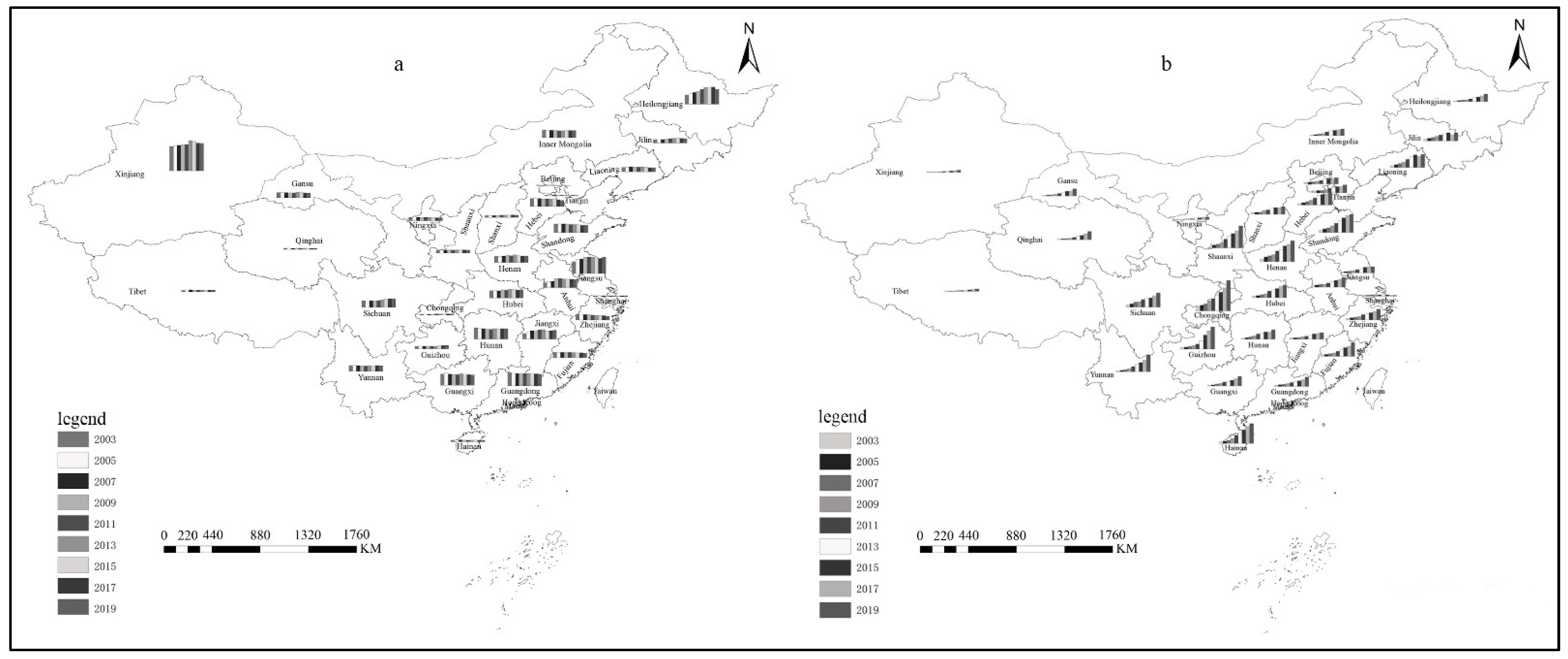
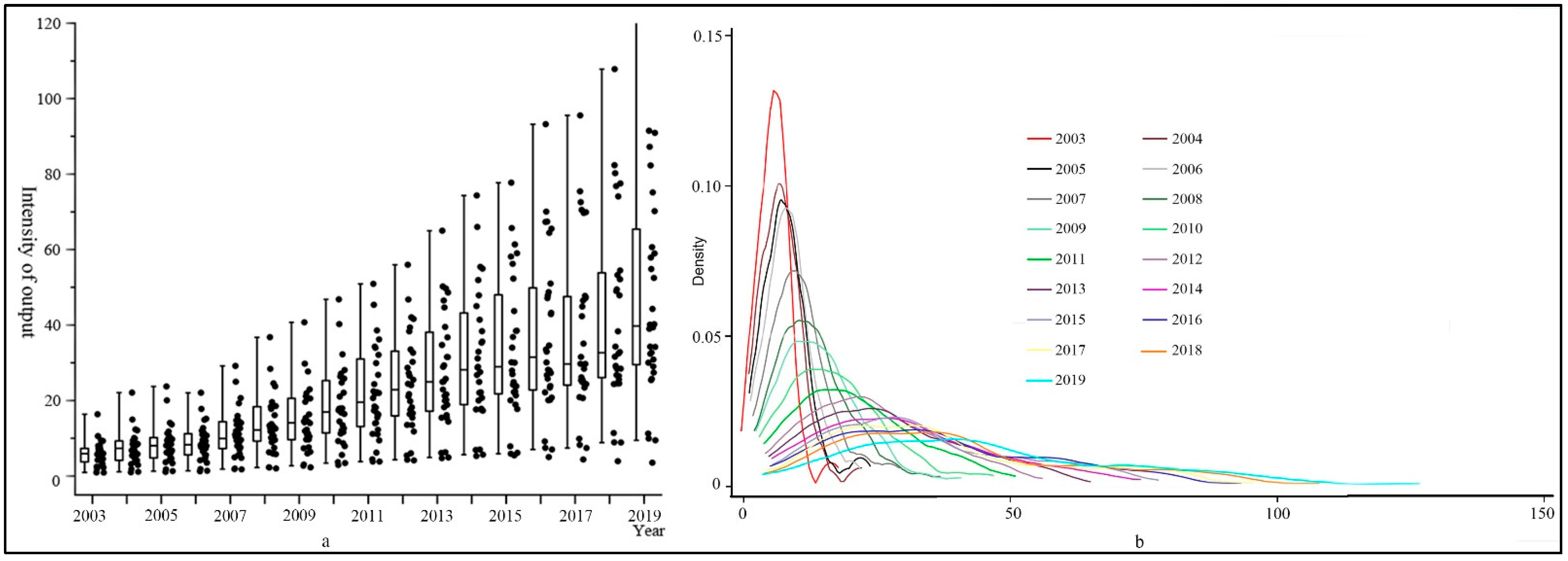
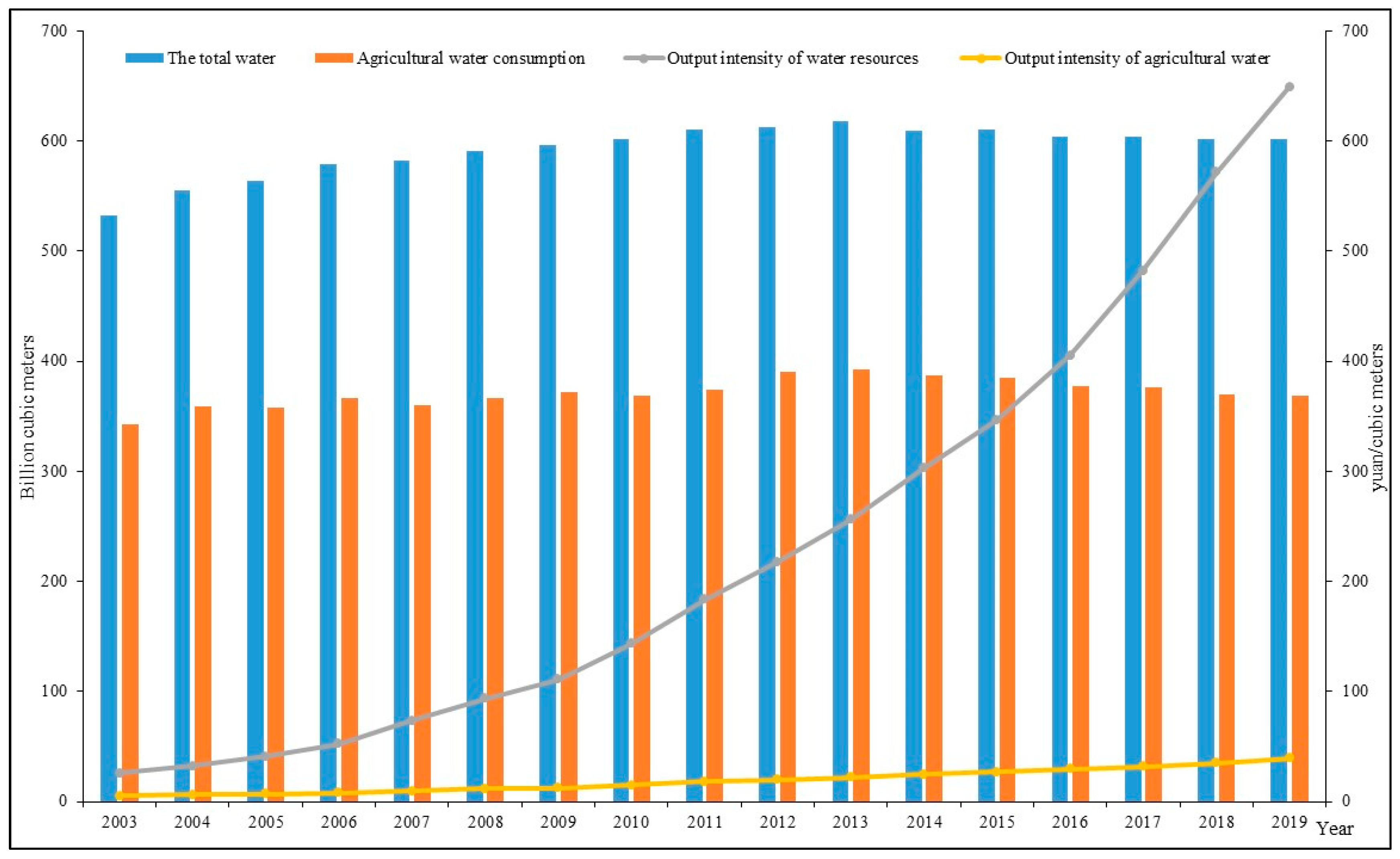
3.1. Spatial and Temporal Sequence Analysis of Output Intensity of Agricultural Water

Figure 1 shows the changes in the total water use, agricultural water use, and output intensity from 2003 to 2019. It can be seen that the total water consumption and agricultural water consumption first experienced an increasing trend and then a decreasing trend during the study period, showing an upward trend from 2003 to 2013 and a downward trend from 2013 to 2019. This is because the Chinese government implemented the “three red lines” restriction policy for agricultural water use in 2010 to achieve effective control over water quantity, efficiency, and quality. The proportion of agricultural water consumption in the amount of total water consumption showed a fluctuating and declining trend. The output intensity of water resources has steadily increased, and, compared to the overall output intensity of water resources, the range of the increase in the agricultural water output intensity was relatively low. Compared to 2003, the overall water output intensity increased by 25 times, while the agricultural water output intensity only increased by seven times; therefore, it is necessary to improve the efficiency of agricultural water use, especially in terms of the effective utilization coefficient of agricultural irrigation water. In 2012, the State Council of the People’s Republic of China issued the “Opinions on Implementing the Strictest Water Resources Management System,” which required the strict implementation of total water consumption control methods, strengthening the management of water use efficiency under the red line and comprehensively promoting the construction of a water-saving society. During the 12th Five-Year Plan period and the 13th Five-Year Plan period, water conservancy departments continued to implement supporting projects for the extension of medium-sized irrigation areas. In addition, they continued to promote the construction of regional large-scale high-efficiency water-saving irrigation projects, increasing the number of high-efficiency water-saving irrigation areas, significantly improving the effective utilization efficiency of farmland irrigation water and improving the effective utilization efficiency of farmland irrigation water.
Figure 2a,b present the changes in the total agricultural water use and agricultural water output intensity for each province in China from 2003 to 2019. As seen in Figure 2a, the total agricultural water consumption in most provinces showed a downward trend during the research period, except for Xinjiang, Heilongjiang, and Sichuan. The provinces with high agricultural water consumption are mainly the eastern and central provinces such as Xinjiang, Heilongjiang, Jiangsu, Guangxi, and Hunan. The average annual agricultural water consumption in these provinces ranges from 12 billion tons to 50 billion tons, with Xinjiang having the largest consumption. These provinces are important grain-producing areas and are important areas that guarantee food security in China. The provinces with low agricultural water consumption are Beijing, Tianjin, Shanghai, and provinces in the western region. The main reason for this low consumption is that the western region has a limited number of water resources, and Beijing, Tianjin, and Shanghai carry out limited agricultural activities. As seen in Figure 2b, the output intensity of agricultural water showed an increasing trend during the study period, with the exception of Shanghai. Chongqing, Henan, Shandong, Shaanxi, Hainan, and other central and eastern provinces have a higher output intensity, with the average production intensity above CNY 30.00/ton and the average production intensity of Chongqing reaching CNY 57.94/ton. This is mainly due to the developed agricultural economy and the high level of agricultural water management in these provinces. The provinces with low agricultural water output intensity are mainly Xinjiang, Tibet, Ningxia, Qinghai, Gansu, and other western regions, which is mainly due to the low level of agricultural economic development and water-saving irrigation agriculture in these regions. Overall, the agricultural water output intensity shows a high spatial pattern in the central parts of the country and a low spatial pattern in the eastern and western parts of the country.
As seen in Figure 3a, during the research period, the intensity of the agricultural water output increased year by year in China; the scattered points of the agricultural water output intensity in different provinces became more and more dispersed, indicating that the differences among provinces were widening. To further understand the distribution of the agricultural water output intensity, a kernel density estimation was carried out to determine the output intensity of agricultural water. The results are shown in Figure 3b. The overall distribution trend of the kernel density curve changes with the curves shifting to the right, indicating that the intensity of the agricultural water output was gradually increasing; a change from a “double peak” to a “single peak” indicates that the differences in agricultural water output intensity between provinces were gradually increasing; a decreasing peak height and increasing peak width indicating that the degree of concentration of the agricultural water output intensity was decreasing in different provinces and that the differences among provinces were increasing; and the tail of the kernel density curve becoming longer, indicating that the number of provinces with high agricultural water output intensity was increasing.

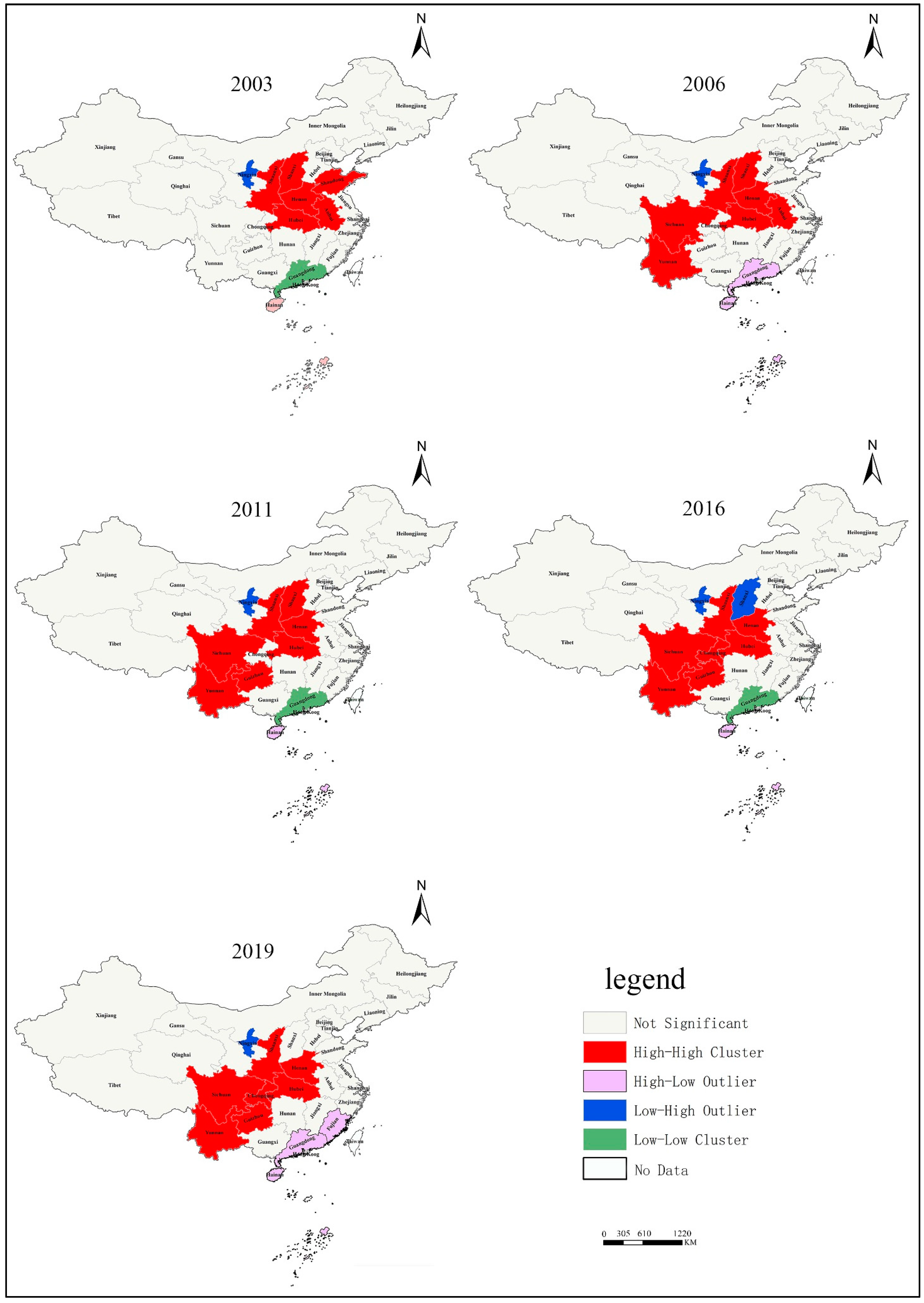
3.2. Spatial Autocorrelation Analysis of Output Intensity of Agricultural Water

Table 2 shows the global Moran I index of the output intensity of agricultural water and the statistical Z-value and P-value from 2003 to 2019. The global Moran I index passed the statistical significance test for Z and P. The Global Moran I index is significantly positive, between 0.2141 and 0.1342, indicating that the output intensity of agricultural water exhibits a significant spatial dispersion trend.
The Global Moran I index reflects the overall spatial correlation characteristics of the output intensity of agricultural water, but it ignores the spatial relationships between partial regions. The spatial pattern characteristics of the output intensity of agricultural water between regions in 2003, 2006, 2011, 2016, and 2019 were visualized with the help of ArcGIS software. Figure 4 shows the local spatial pattern characteristics of the output intensity of agricultural water. The local spatial pattern was relatively stable, with the high–high agglomeration areas mainly being distributed in Southwest China and Central China And shown to be expanding. The low–high agglomeration areas were mainly concentrated around Shaanxi Province, and the low–high agglomeration areas were relatively stable. Guangdong Province changed between being a high–low agglomeration and low–low agglomeration area. Hainan Province has always been in a high–low agglomeration area. The results show that the local spatial patterns of the output intensity of agricultural water have mostly been stable since 2011.

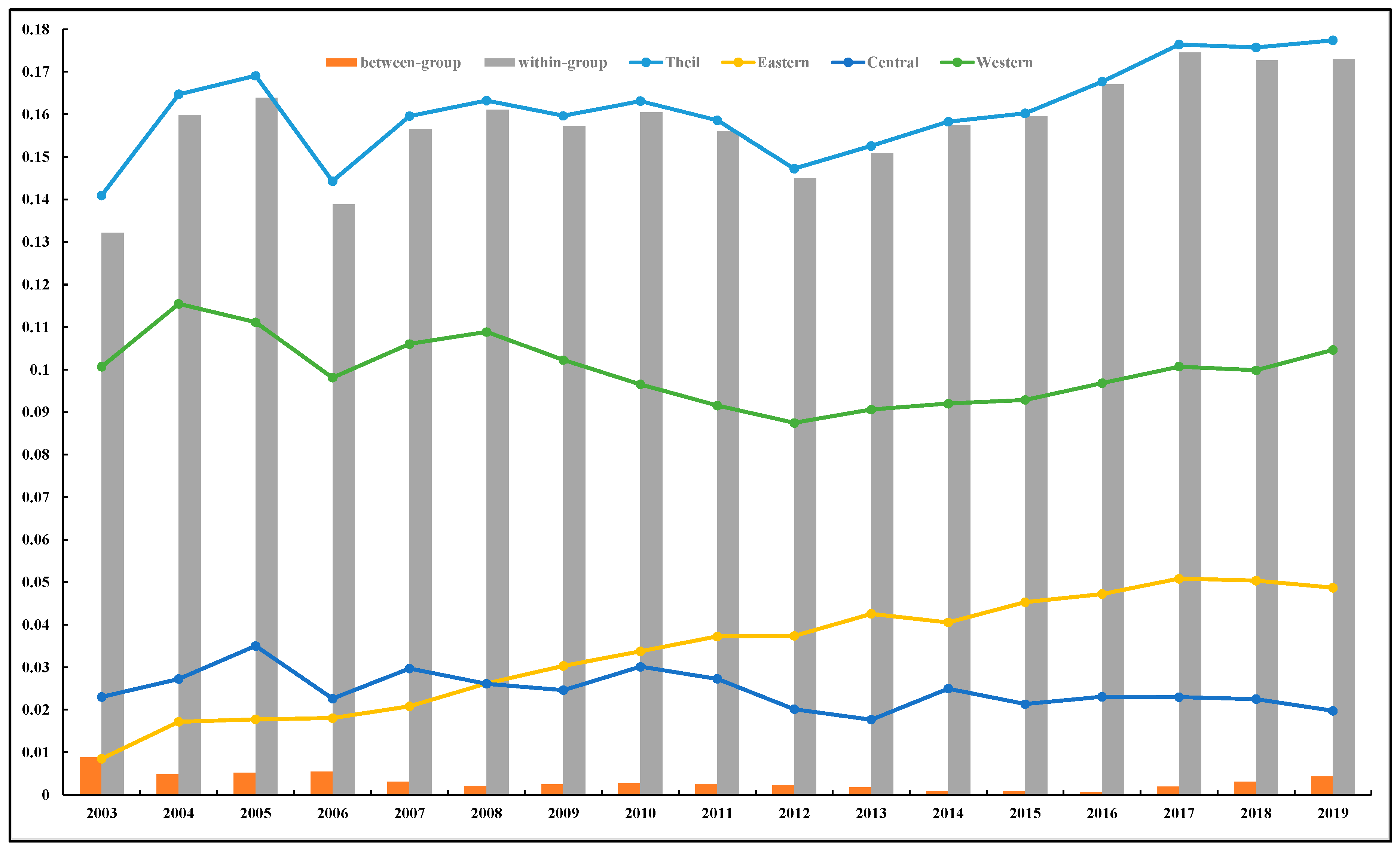
3.3. Analysis of Regional Differences of Output Intensity of Agricultural Water

To ensure the accuracy of the results, we calculated the Gini coefficient and the Theil index to verify each other. According to Figure 5, the Gini coefficient and Theil index show similar trends during the study period. The Gini coefficient and Theil index showed M-shaped change characteristics from 2003 to 2012 and showed a slight upward trend, but the changes were not significant; the Gini coefficient and Theil index showed a significant upward trend from 2012 to 2019. During the entire study period, the growth rate of the Gini coefficient and Theil index showed the same increasing or decreasing trend, indicating that although the changes in the output intensity of agricultural water were different in different provinces, the regional differences had the same change trends. The growth rate of the Gini coefficient and Theil index underwent the largest changes in 2004 and 2006, respectively, but both achieved their maximum value in 2019. While the Gini coefficient and Theil index were increasing, their growth rates were falling, suggesting that while regional differences were growing, the rate at which they were widening was slowing down. Throughout the study period, the Gini coefficient remained larger than the Theil index. The Gini coefficient was more sensitive to changes in the middle values, and the Theil index was more sensitive to changes in the values at both ends [24,35]. Therefore, we can determine that medium-level changes in the output intensity of agricultural water in provinces are stronger than they are in provinces with high-level and low-level changes.
In addition, we compared the changes in the Gini coefficient, Theil index, and Moran index, and we could see that the change trends in the Moran index were completely opposite to those of the Gini coefficient and Theil index. It also indicated that the overall difference was increasing during the study period.
To reveal the differences in the output intensity of agricultural water in eastern, central, and western China, we decomposed the Theil index using the formula. As seen in Figure 6, the within-group Theil index of the output intensity of agricultural water had the same trend as the overall Theil index, and the within-group differences were much larger than the between-group differences. The within-group Theil index accounted for more than 98% of the overall Theil index, indicating that the overall difference was mainly dominated by within-group differences. The within-group Theil index increased from 0.1322 in 2013 to 0.1731 in 2019, with an average annual increase of 1.98%. The between-group Theil index first showed a decreasing trend and then an increasing trend, but a decreasing trend overall.
At the regional level, the Theil index was the largest in the western region, followed by the eastern and central regions, with mean values of 0.099, 0.034, and 0.025, respectively. The Theil index in the eastern region showed an increasing trend during the study period and increased from 0.0085 in 2003 to 0.0487 in 2019, with an annual increase of 13.4%. The Theil index in the central region showed a fluctuating downward trend during the study period and decreased from 0.023 in 2003 to 0.019 in 2019. In the western region, the Theil index showed a decreasing trend and then an increasing trend during the study period, reaching its minimum value in 2012 and then rising, indicating that the difference in the western region was the lowest in 2012. After 2021 the difference began to increase. In the western region, the trend of the Theil index was like that of the overall Theil index and the within-group Theil index, and the Theil index in the western region accounted for 61.9% of the overall Theil index and 63.12% of the within-group Theil index, indicating that the differences in the western region affected the overall difference.

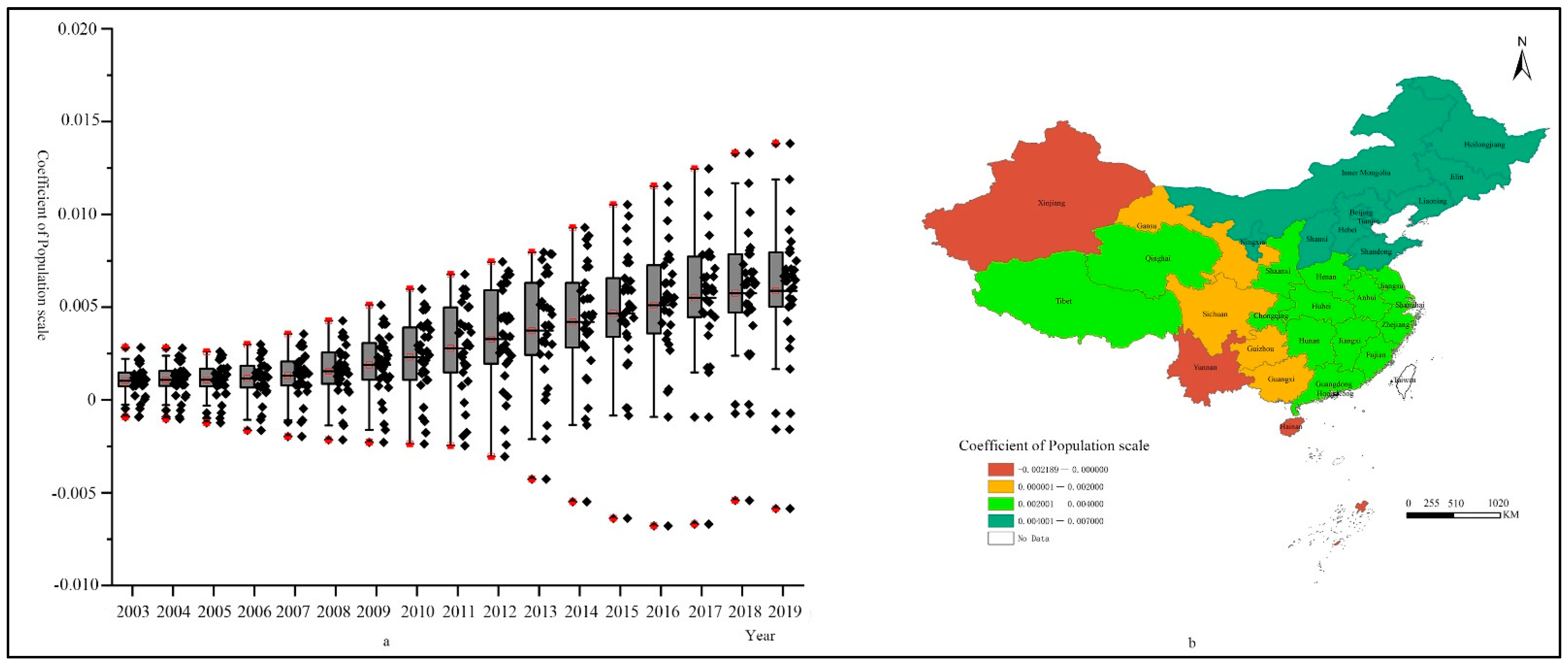
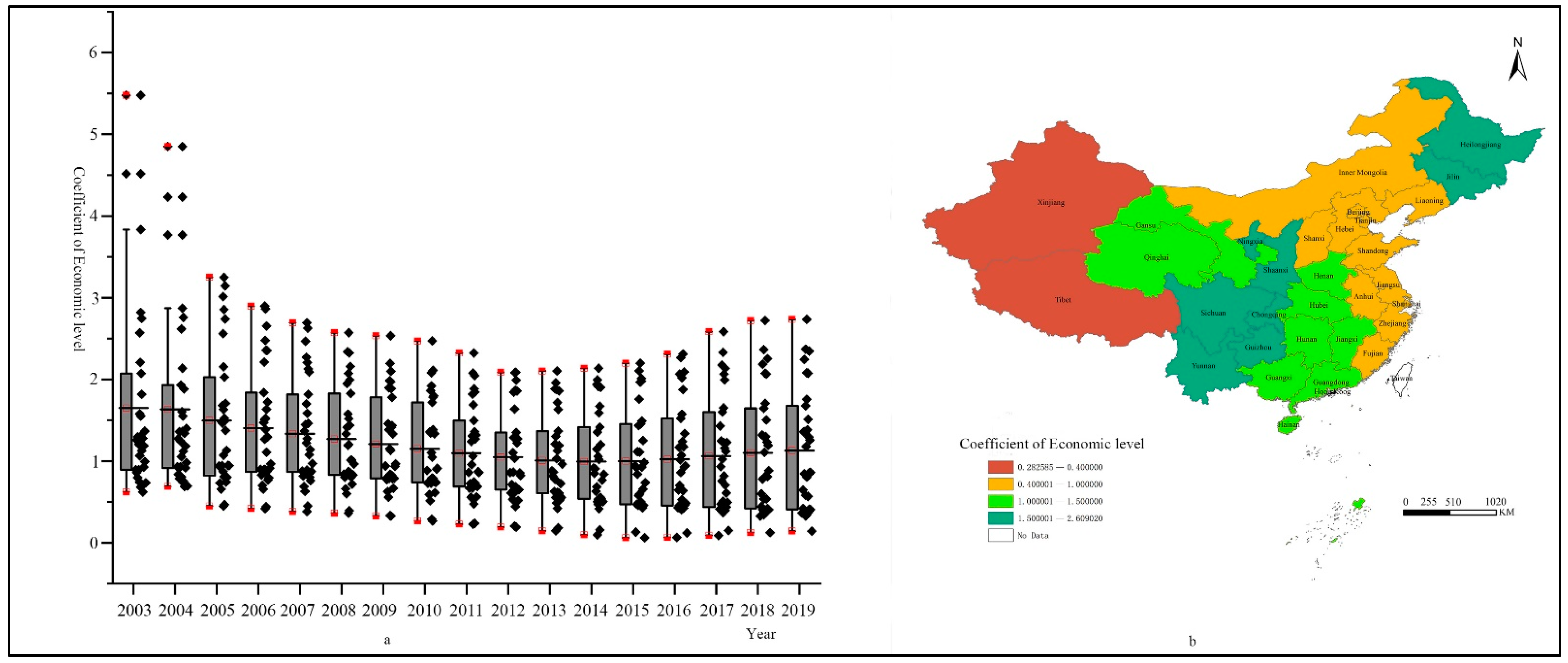
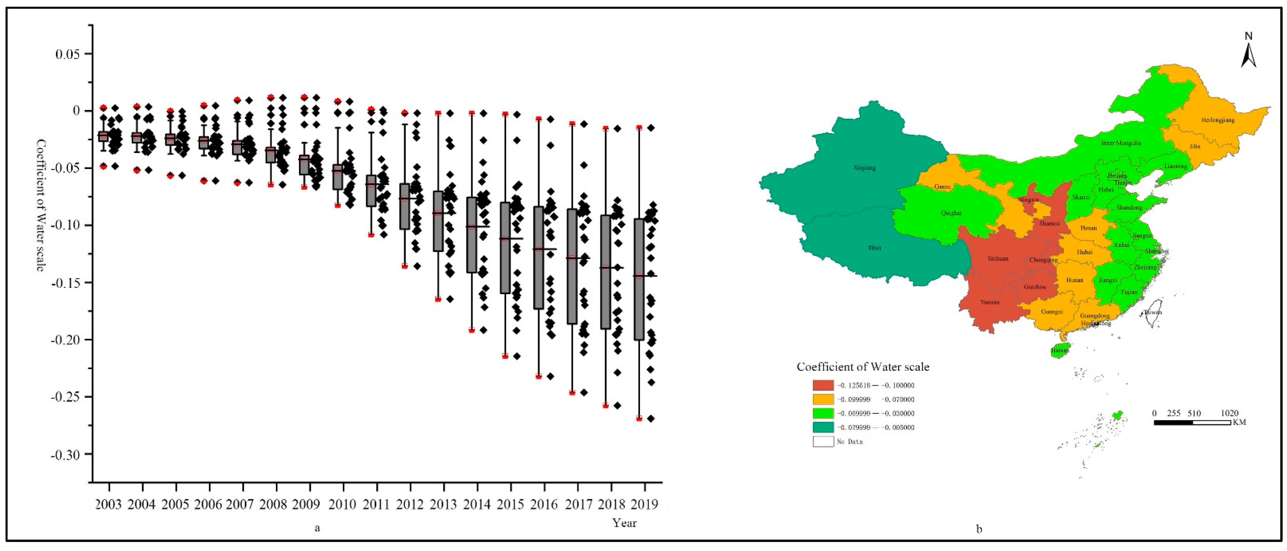
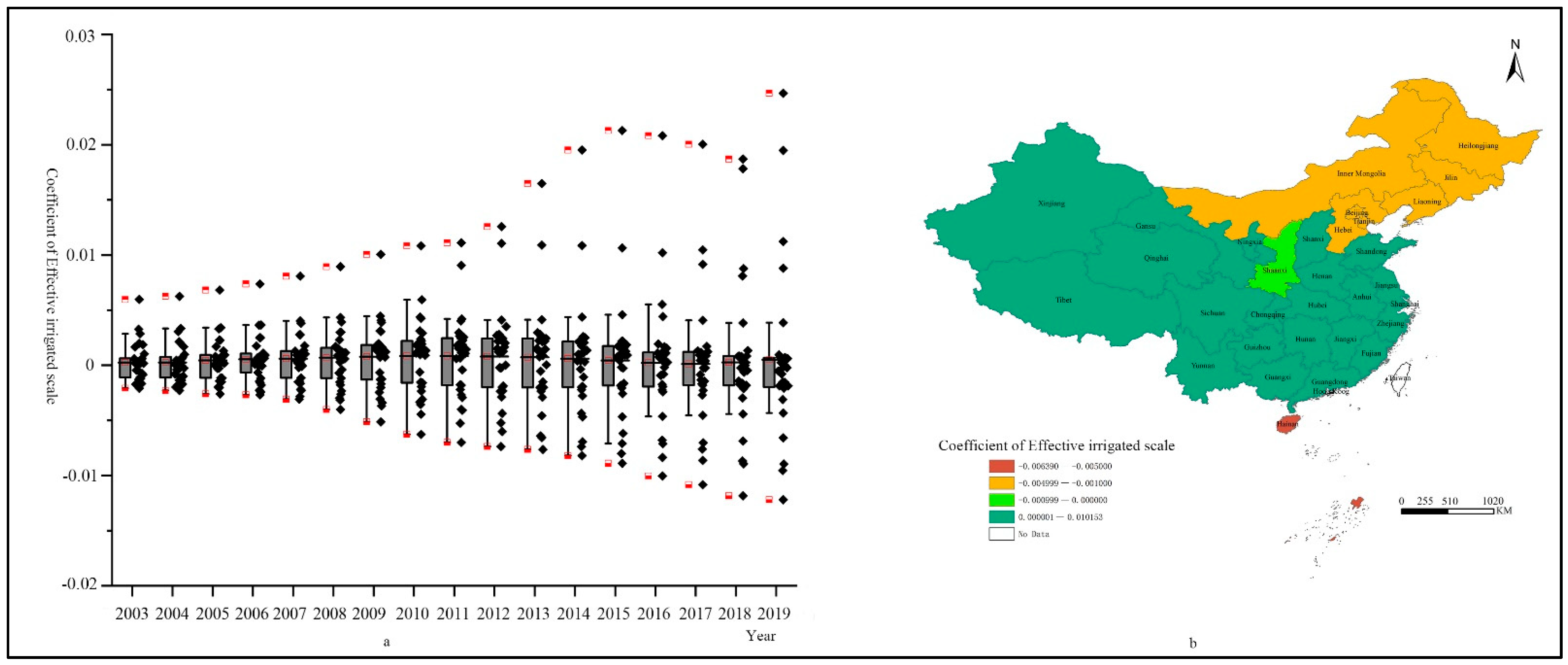
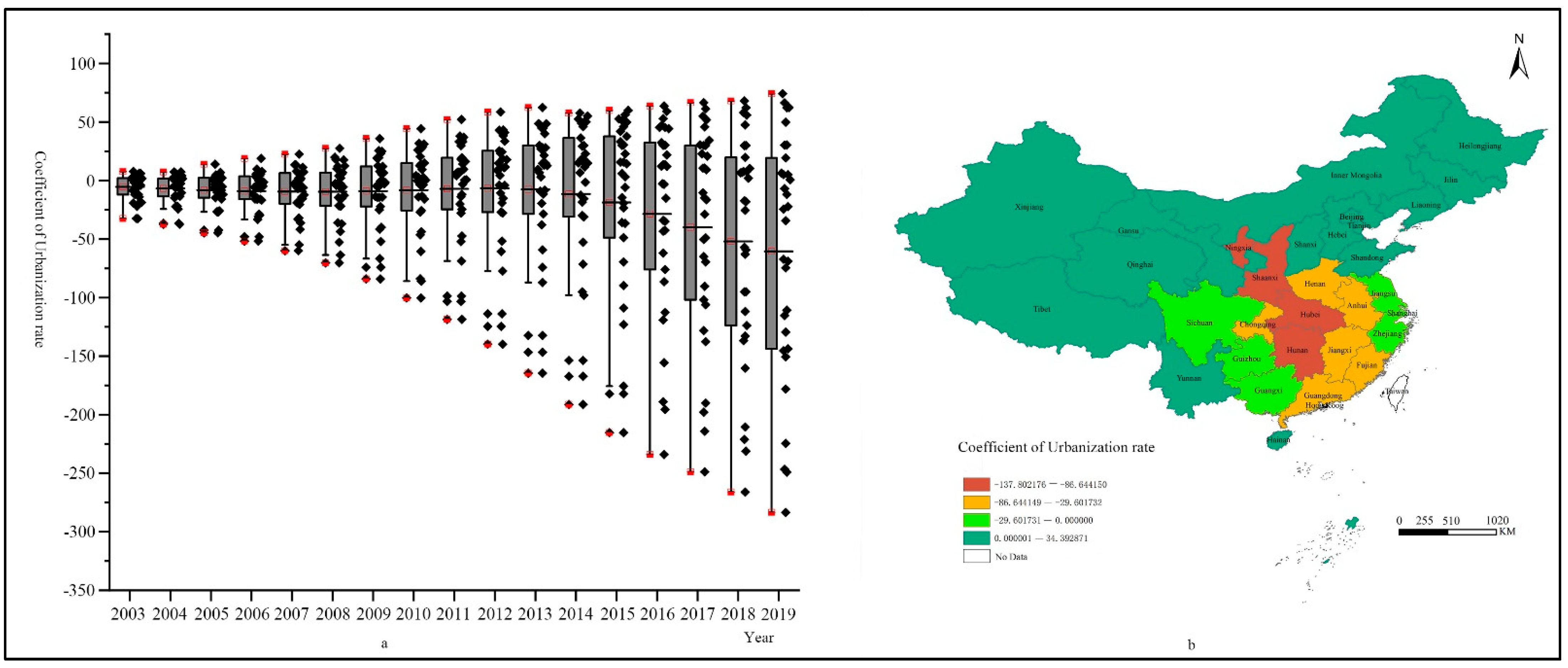
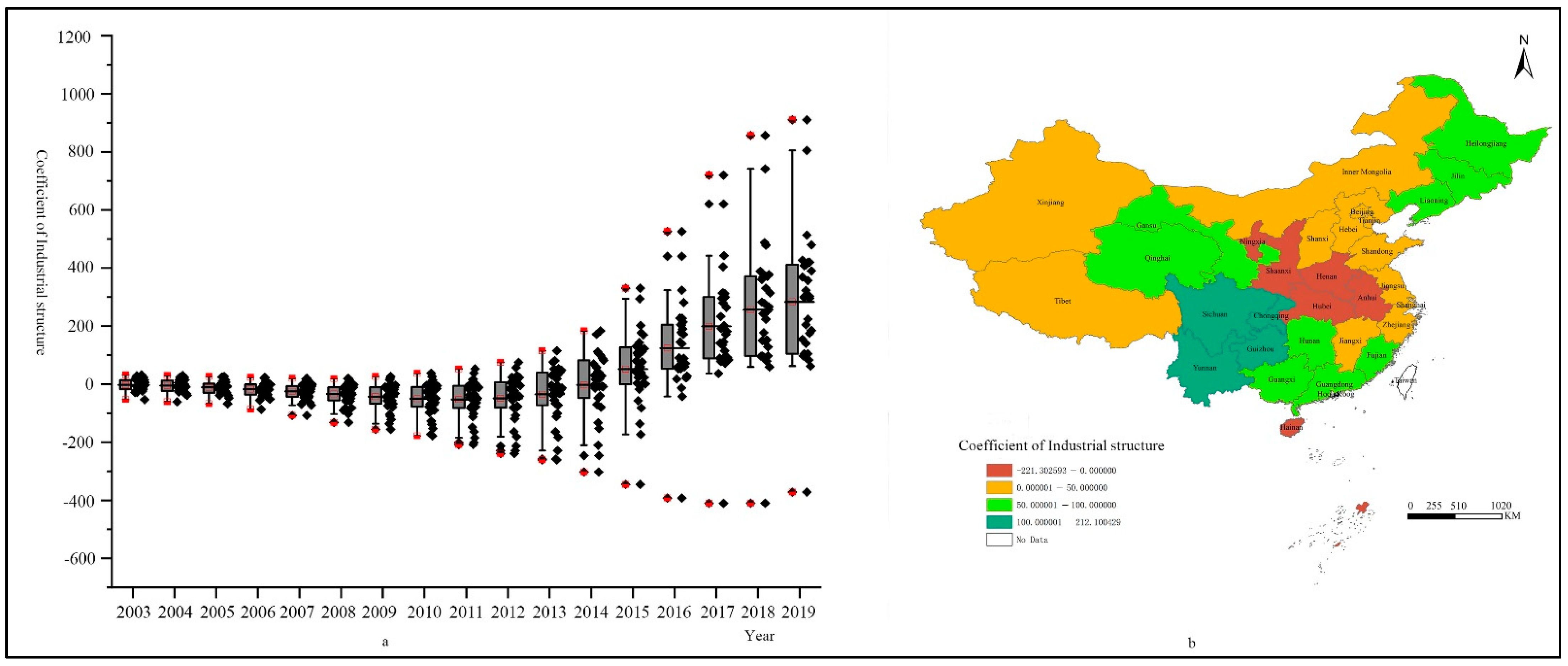
3.4. Temporal and Spatial Analysis of Influencing Factors

In order to avoid the influence of multiple collinearities among the independent variables during the regression estimation, this study carried out multiple collinearity tests on the variables, and the results are shown in Table 3. We found that the variance inflation factor was less than ten and that the tolerance was greater than 0.1, indicating no multiple collinearities among the explanatory variables [36,37,38], meaning that we could conduct regression analysis.
To further analyze the temporal and spatial differences influencing different explanatory variables during different periods on the agricultural water output intensity at the provincial level, the GTWR, GWR, and TWR were used for analysis. We chose the best model by comparing the residual squares, AICc, R2, and adjusted R2 [38,39,40]. By comparing these three models in Table 4, we found that the R2 and adjusted R2 of GTWR were the largest, 0.9734 and 0.9731, while the residual squares and AICc were the smallest at 5432.44 and 2940.74; therefore, the interpretation effect of the GTWR model was the best.
In this study, the GTWR model was used to estimate the influence of various factors on the output intensity of agricultural water in different provinces during different periods. At the same time, the mean value of the regression coefficient of each influencing factor in each province was used for spatial expression to analyze the spatial difference of each influencing factor.
Figure 7 reveals that the population scale had a positive promotion effect and improved the output intensity of the agricultural water during the study period year by year, with the average regression coefficient of the population scale being 0.0031. As the size of the population increases, industrial, domestic, and ecological water use also increase, crowding out part of the water that has traditionally been used in agriculture. However, as the population increases, the demand for food also increases, encouraging the promotion and application of water-saving irrigation technology, further improving water efficiency, increasing the marginal output of water resources, and thus improving the output intensity of agricultural water. From the perspective of spatial distribution, the scale of the population in the eastern and central regions had a positive promoting effect on the output intensity of agricultural water. In contrast, the population scale in the western regions (with the exception of Tibet and Qinghai) had little effect on the output intensity of agricultural water, and there was a negative correlation in Xinjiang, Yunnan, and Hainan. This was mainly because the western regions are the main areas for population migration in China; moreover, the agricultural production conditions are relatively poor, as these regions are in arid and semi-arid regions.
Figure 8 shows that the economic level had a positive effect on the output intensity of agricultural water, and the average regression coefficient of the economic level was 1.2116. However, as the economic level improved, an inverted U-shaped curve appeared, which first decreased and then increased. The total agricultural water consumption increased year by year from 2003 to 2013, promoting the improvement of the economic development level. However, after 2013, the total agricultural water use showed a downward trend because of the improvement of the economic development level, the gradual optimization of the economic development model, and the implementation of the total amount and intensity control targets. The promotion of water-saving projects and technologies, in addition to the reasons previously mentioned, improved the output intensity of agricultural water. From the spatial distribution of the influence of the economic level on the output intensity of agricultural water, the difference in the impact of the economic level on the western region was relatively obvious and had the least amount of impact on Xinjiang and Tibet and a moderate amount of impact on Gansu and Qinghai. In other western provinces, the impact had a significant positive promoting effect. This is because the gap in the economic development level is larger between provinces in western China, further showing that the level of economic development has an obvious impact on the output intensity of agricultural water. The promoting effect on the central region was stronger than that of the eastern region, but no obvious different were observed within the region. This is mainly because the central region is the main agricultural development region in China. As the level of economic development improves, local governments have a greater capacity to invest more in horizontal facilities, thus improving the output intensity of agricultural water.
Figure 9 shows that the water use scale had a negative impact on the regional output intensity of agricultural water. The average regression coefficient of the water use scale was −0.0721 and showed that the downward trend of the regression coefficient was intensifying. This is because the expansion of the water use scale may inhibit the application of water-saving technology, and China’s price for agricultural water is relatively low. This leads to the water set aside for agriculture being wasted. From the perspective of spatial distribution, the influence of the water use scale on the output intensity of agricultural water presented a block distribution characteristic, and great differences were observed within the western and central regions; the eastern regions were relatively consistent within the region. The total water consumption had the most significant negative effect on the output intensity of agricultural water in southwest China. The main reason for this is that the water situation is very different in different parts of China, as water reforms are still at their initial stages.
Figure 10 shows that the impact of the water use structure had both positive and negative effects on the regional output intensity of agricultural water, indicating that the water use structure in some areas was optimized and reasonable, effectively promoting the regional output intensity of agricultural water. With the development of the agricultural economy, agricultural water consumption continued to increase, and the regression coefficient of agricultural water use structure continued to rise. However, after the total amount of control target was proposed, the trend of the regression coefficient began to decline gradually and even appeared to have a negative influence. The main reason for this is that with the control of total water consumption, the proportion of ecological water and domestic water is increasing year by year, reducing the proportion of agricultural water. Therefore, determining a reasonable proportion of agricultural water and improving the use efficiency of agricultural water have had positive significance for improving the output intensity of agricultural water. In terms of the spatial distribution, the regression coefficient of the central and western regions was negative, while that of the eastern regions was positive. The proportion of agricultural water in central and western provinces was relatively high. However, the efficiency of agricultural water was lower than it was in the eastern provinces [41], indicating that agricultural water waste was a serious problem in the agricultural production process in the central and western regions. Therefore, the agricultural water efficiency should be improved under the conditions of comprehensive water control. This is especially true in the central region because the central region represents an important grain-producing area in China.
As shown in Figure 11, the effective irrigation scale had both positive and negative effects on the regional output intensity of agricultural water, but the degree of influence was not obvious, and the average regression coefficient was only 0.0005. Effective farmland irrigation was large in China, but the effect of effective irrigation on the agricultural water output intensity was not obvious. Therefore, the management department should promote the modernization of irrigation areas and build water-saving irrigation areas. During the irrigation process, the total amount of irrigation water should follow quota management requirements. Each province should determine its effective irrigation scale according to agricultural water consumption. At the regional level, the average regression coefficients of most of the provinces in China were positive, except for northeast and northern China.
Figure 12 shows that urbanization had a positive and negative impact on the output intensity of agricultural water; over time, the number of provinces with negative impacts increased, and the degree of negative impact gradually became stronger. As urbanization and industrialization continue to increase, industrial and domestic water use will also continue to increase, which will crowd out agricultural water use. Agricultural water resources are seriously affected by urbanization, which has become one of the important factors restricting the sustainable development of agriculture [42,43]. Based on the permanent urban population, the urbanization rate has increased from 17.92% in 1978 to 60.60% in 2019 [44]. The long-term impacts of urbanization on agricultural water consumption are as follows: the increase in the urban population will increase urban domestic water consumption, and the reduction in the number of agricultural employees will distort the allocation of agricultural production resources and reduce the output intensity of agricultural water [45]. From the perspective of spatial distribution, the impact of urbanization on the output intensity of agricultural water showed characteristics of north–south differentiation, with the urbanization in northern China having a positive impact, and a negative impact in southern China. In the southern region, the negative influence from the center to the periphery decreased.
Figure 13 shows that the impact of industrial structure on the output intensity of agricultural water was positive. The average regression coefficient of the industrial structure showed an obvious upward trend, indicating that the output intensity of agricultural water would increase as the added value of agriculture increased. This was because, with the implementation of relevant water resource management policies, agricultural water consumption declined. However, the agricultural added value grew steadily, and the level of growth experienced by the output intensity was better than the decline in the industrial structure. Therefore, the industrial structure had a positive promoting effect on the output intensity of agricultural water. In terms of spatial distribution, industrial structure played a positive role. There was an obvious spatial agglomeration phenomenon. The most significant promoting effect was observed in Southwest China, followed by Southeast China, Northeast China, and, finally, North China, with an inhibiting effect observed in Ningxia, Shaanxi, Henan, Hubei, Anhui, and Hainan.

4. Conclusions and Policy Implications

Based on the data from 31 Chinese provinces from 2003 to 2019, we analyzed the regional differences and factors influencing the agricultural water output intensity in China. First, the temporal and spatial distribution characteristics of the agricultural water output intensity in China were analyzed. Second, a spatial autocorrelation analysis was carried out. Third, we evaluated the regional inequality of the agricultural water output intensity among the different provinces. Finally, the effects of population scale, economic level, water use scale, water use structure, effective irrigation scale, urbanization, and industrial structure on the agricultural water output intensity were discussed. The main conclusions of this study are as follows: (1) The total water consumption and agricultural water consumption first experienced an increasing and then a decreasing trend during the study period. The output intensity of the water resources showed a steady increase. Compared to the overall output intensity of the water resources, the increased range of the agricultural water output intensity was relatively low. Compared to 2003, overall water output intensity increased by 25 times, while the agricultural water output intensity only increased seven times. The provinces with high agricultural water consumption were the eastern and central provinces, and the provinces with a high output intensity of agricultural water were also concentrated in the central and eastern regions. (2) By calculating the global Moran index, we found that the output intensity of agricultural water exhibited a significant spatial dispersion trend. By analyzing the local autocorrelation, it was found that a local spatial agglomeration phenomenon existed and that the pattern of local spatial agglomeration was relatively stable. (3) The paper applied the Gini coefficient and Theil index to estimate the regional differences in the output intensity of agricultural water. We found that the overall difference in the output intensity of agricultural water in China was increasing but also that the widening trend was being alleviated. The main reason for the increase in the overall differences was that the intra-group differences among the three regions were increasing, with the largest intra-group differences being observed in the western region, followed by the eastern region and the central region. (4) The GTWR model was used to analyze the influence of the factors influencing the output intensity of agricultural water. We found that population scale, water use scale, water use structure, effective irrigation scale, urbanization, and industrial structure had significant spatial differences on the output intensity of agricultural water but that the level of economic development had a positive impact on the agricultural water output intensity of all the studied provinces.
The effective utilization coefficient of agricultural water was low in China. During agricultural development, it is not only necessary to strictly control the total amount of water resources but also to improve the efficiency of water resource utilization, improve the output intensity of water resources, ensure food security, and promote the sustainable development of agriculture. According to the study’s conclusion, the government should not only consider the overall utilization of water resources but should also consider regional differentiation when making water resource management policies. Different water resources utilization policies should be formulated according to the regional differences in the output intensity of agricultural water. Different regions and provinces should formulate water resource policies that align with the actual level of regional development according to the different effects of the factors influencing the output intensity of agricultural water.

Author Contributions

J.P.: conceptualization, methodology, software, writing—original draft, funding acquisition; X.L. (Xue Li) and X.L. (Xiang Li): writing—original draft, data curation; T.Y.: data curation; Y.L.: writing—original draft; X.C.: conceptualization. All authors have read and agreed to the published version of the manuscript.

Funding

This research was supported by the grant from the National Key R&D Program of China (2018YFC0704702) and was supported by the Fundamental Research Funds for the Central Universities of Lanzhou University (2020jbkyzy032, 2019jbkyjd014).

Institutional Review Board Statement

Not applicable.

Informed Consent Statement

Not Applicable.

Data Availability Statement

The authors may provide raw data if necessary.

Conflicts of Interest

The authors declare no conflict of interest. This article does not contain any studies with human participants or animals performed by any of the authors. Informed consent was obtained from all individual participants included in the study.

References

  1. D’Odorico, P.; Chiarelli, D.D.; Rosa, L.; Bini, A.; Zilberman, D.; Rulli, M.C. The global value of water in agriculture. Proc. Natl. Acad. Sci. USA 2020, 117, 21985–21993. [Google Scholar] [CrossRef] [PubMed]
  2. Sun, S.K.; Yin, Y.L.; Wu, P.T.; Wang, Y.B.; Luan, X.B.; Li, C. Geographical Evolution of Agricultural Production in China and Its Effects on Water Stress, Economy, and the Environment: The Virtual Water Perspective. Water Resour. Res. 2019, 55, 4014–4029. [Google Scholar] [CrossRef]
  3. Kang, S.; Hao, X.; Du, T.; Tong, L.; Su, X.; Lu, H.; Li, X.; Huo, Z.; Li, S.; Ding, R. Improving agricultural water productivity to ensure food security in China under changing environment: From research to practice. Agric. Water Manag. 2017, 179, 5–17. [Google Scholar] [CrossRef]
  4. Wang, S.; Hu, Y.; Yuan, R.; Feng, W.; Pan, Y.; Yang, Y. Ensuring water security, food security, and clean water in the North China Plain-conflicting strategies. Curr. Opin. Environ. Sustain. 2019, 40, 63–71. [Google Scholar] [CrossRef]
  5. Huai, H.; Chen, X.; Huang, J.; Chen, F. Water-Scarcity Footprint Associated with Crop Expansion in Northeast China: A Case Study Based on AquaCrop Modeling. Water 2020, 12, 125. [Google Scholar] [CrossRef] [Green Version]
  6. Entezari, A.; Wang, R.Z.; Zhao, S.; Mahdinia, E.; Wang, J.Y.; Tu, Y.D.; Huang, D.F. Sustainable agriculture for water-stressed regions by air-water-energy management. Energy 2019, 181, 1121–1128. [Google Scholar] [CrossRef]
  7. Hoekstra, A.Y.; Mekonnen, M.M. The water footprint of humanity. Proc. Natl. Acad. Sci. USA 2012, 109, 3232–3237. [Google Scholar] [CrossRef] [Green Version]
  8. Wheeler, T.; Von Braun, J. Climate Change Impacts on Global Food Security. Science 2013, 341, 508–513. [Google Scholar] [CrossRef]
  9. Brauman, K.A.; Siebert, S.; Foley, J.A. Improvements in crop water productivity increase water sustainability and food security-a global analysis. Environ. Res. Lett. 2013, 8, 024032. [Google Scholar] [CrossRef]
  10. Li, K.; Liang, S.; Liang, Y.; Feng, C.; Qi, J.; Xu, L.; Yang, Z. Mapping spatial supply chain paths for embodied water flows driven by food demand in China. Sci. Total Environ. 2021, 786, 147480. [Google Scholar] [CrossRef]
  11. Zhai, Y.; Zhang, T.; Bai, Y.; Ji, C.; Ma, X.; Shen, X.; Hong, J. Energy and water footprints of cereal production in China. Resour. Conserv. Recycl. 2021, 164, 105150. [Google Scholar] [CrossRef]
  12. Sun, S.K.; Wu, P.T.; Wang, Y.B.; Zhao, X.N. The virtual water content of major grain crops and virtual water flows between regions in China. J. Sci. Food Agric. 2013, 93, 1427–1437. [Google Scholar] [CrossRef] [PubMed]
  13. Siebert, S.; Kummu, M.; Porkka, M.; Döll, P.; Ramankutty, N.; Scanlon, B.R. A global data set of the extent of irrigated land from 1900 to 2005. Hydrol. Earth Syst. Sci. 2015, 19, 1521–1545. [Google Scholar] [CrossRef] [Green Version]
  14. Awume, O.; Patrick, R.; Baijius, W. Indigenous Perspectives on Water Security in Saskatchewan, Canada. Water 2020, 12, 810. [Google Scholar] [CrossRef] [Green Version]
  15. Jin, H.; Huang, S. Are China’s Water Resources for Agriculture Sustainable? Evidence from Hubei Province. Sustainability 2021, 13, 3510. [Google Scholar] [CrossRef]
  16. Yin, L.; Tao, F.; Chen, Y.; Wang, Y. Reducing agriculture irrigation water consumption through reshaping cropping systems across China. Agric. For. Meteorol. 2022, 312, 108707. [Google Scholar] [CrossRef]
  17. Wei, J.; Lei, Y.; Yao, H.; Ge, J.; Wu, S.; Liu, L. Estimation and influencing factors of agricultural water efficiency in the Yellow River basin, China. J. Clean. Prod. 2021, 308, 127249. [Google Scholar] [CrossRef]
  18. Guo, S.; Shen, G.Q.; Peng, Y. Embodied agricultural water use in China from 1997 to 2010. J. Clean. Prod. 2016, 112, 3176–3184. [Google Scholar] [CrossRef] [Green Version]
  19. Zhang, H.; Zhou, Q.; Zhang, C. Evaluation of agricultural water-saving effects in the context of water rights trading: An empirical study from China’s water rights pilots. J. Clean. Prod. 2021, 313, 127725. [Google Scholar] [CrossRef]
  20. He, Y.; Wang, Y.; Chen, X. Spatial patterns and regional differences of inequality in water resources exploitation in China. J. Clean. Prod. 2019, 227, 835–848. [Google Scholar] [CrossRef]
  21. Jiang, L.; Yu, L.; Xue, B.; Chen, X.; Mi, Z. Who is energy poor? Evidence from the least developed regions in China. Energy Policy 2020, 137, 111122. [Google Scholar] [CrossRef]
  22. Malakar, K.; Mishra, T.; Patwardhan, A. Inequality in water supply in India: An assessment using the Gini and Theil indices. Environ. Dev. Sustain. 2018, 20, 841–864. [Google Scholar] [CrossRef]
  23. Pang, J.; Li, H.; Lu, C.; Lu, C.; Chen, X. Regional Differences and Dynamic Evolution of Carbon Emission Intensity of Agriculture Production in China. Int. J. Environ. Res. Public Health 2020, 17, 7541. [Google Scholar] [CrossRef]
  24. Liu, J.; Li, S.; Ji, Q. Regional differences and driving factors analysis of carbon emission intensity from transport sector in China. Energy 2021, 224, 120178. [Google Scholar] [CrossRef]
  25. Chen, J.; Xu, C.; Cui, L.; Huang, S.; Song, M. Driving factors of CO2 emissions and inequality characteristics in China: A combined decomposition approach. Energy Econ. 2019, 78, 589–597. [Google Scholar] [CrossRef]
  26. Xu, C. Determinants of carbon inequality in China from static and dynamic perspectives. J. Clean. Prod. 2020, 277, 123286. [Google Scholar] [CrossRef]
  27. Zhang, Z.; Han, W.; Chen, X.; Yang, N.; Lu, C.; Wang, Y. The Life-Cycle Environmental Impact of Recycling of Restaurant Food Waste in Lanzhou, China. Appl. Sci. 2019, 9, 3608. [Google Scholar] [CrossRef] [Green Version]
  28. Ren, J.; Lyu, D.; Chen, X.; Liu, P.; Guan, D.; Su, K.; Zhang, H. Oblique extension of pre-existing structures and its control on oil accumulation in eastern Bohai Sea. Pet. Explor. Dev. 2019, 46, 553–564. [Google Scholar] [CrossRef]
  29. Zhang, L.; Pang, J.; Chen, X.; Lu, Z. Carbon emissions, energy consumption and economic growth: Evidence from the agricultural sector of China’s main grain-producing areas. Sci. Total Environ. 2019, 665, 1017–1025. [Google Scholar] [CrossRef]
  30. Wang, H.; Pan, X.; Zhang, S. Spatial autocorrelation, influencing factors and temporal distribution of the construction and demolition waste disposal industry. Waste Manag. 2021, 127, 158–167. [Google Scholar] [CrossRef]
  31. Huang, B.; Wu, B.; Barry, M. Geographically and temporally weighted regression for modeling spatio-temporal variation in house prices. Int. J. Geogr. Inf. Sci. 2010, 24, 383–401. [Google Scholar] [CrossRef]
  32. Wu, D. Spatially and temporally varying relationships between ecological footprint and influencing factors in China’s provinces Using Geographically Weighted Regression (GWR). J. Clean. Prod. 2020, 261, 121089. [Google Scholar] [CrossRef]
  33. Wu, B.; Li, R.; Huang, B. A geographically and temporally weighted autoregressive model with application to housing prices. Int. J. Geogr. Inf. Sci. 2014, 28, 1186–1204. [Google Scholar] [CrossRef]
  34. Chu, H.J.; Huang, B.; Lin, C.Y. Modeling the spatio-temporal heterogeneity in the PM10-PM2.5 relationship. Atmos. Environ. 2015, 102, 176–182. [Google Scholar] [CrossRef]
  35. Atkinson, A. On the measurement of inequality. J. Econ. Theory 1970, 2, 244–263. [Google Scholar] [CrossRef]
  36. Sheng, J.; Han, X.; Zhou, H. Spatially varying patterns of afforestation/reforestation and socio-economic factors in China: A geographically weighted regression approach. J. Clean. Prod. 2017, 153, 362–371. [Google Scholar] [CrossRef]
  37. Wang, Y.; Chen, W.; Kang, Y.; Li, W.; Guo, F. Spatial correlation of factors affecting CO2 emission at provincial level in China: A geographically weighted regression approach. J. Clean. Prod. 2018, 184, 929–937. [Google Scholar] [CrossRef]
  38. Sá, A.C.; Pereira, J.; Charlton, M.E.; Mota, B.; Barbosa, P.M.; Stewart Fotheringham, A. The pyrogeography of sub-Saharan Africa: A study of the spatial non-stationarity of fire-environment relationships using GWR. J. Geogr. Syst. 2011, 13, 227–248. [Google Scholar] [CrossRef] [Green Version]
  39. Mcmillen, D.P. Geographically weighted regression: The analysis of spatially varying relationships. Am. J. Agric. Econ. 2004, 86, 554–556. [Google Scholar] [CrossRef]
  40. O’Sullivan, D. Geographically weighted regression: The analysis of spatially varying relationships. Geogr. Anal. 2003, 35, 272–275. [Google Scholar] [CrossRef]
  41. Wang, F.; Yu, C.; Xiong, L.; Chang, Y. How can agricultural water use efficiency be promoted in China? A spatial-temporal analysis. Resour. Conserv. Recycl. 2019, 145, 411–418. [Google Scholar] [CrossRef]
  42. Feng, G.Z. Impacts of and Solutions to Urbanization on Agricultural Water Resources. Ph.D. Thesis, Colorado State University, Fort Collins, CO, USA, 2000. [Google Scholar]
  43. Avazdahandeh, S.; Khalilian, S. The effect of urbanization on agricultural water consumption and production: The extended positive mathematical programming approach. Environ. Geochem. Health 2021, 43, 247–258. [Google Scholar] [CrossRef] [PubMed]
  44. Lu, W.; Sarkar, A.; Hou, M.; Liu, W.; Guo, X.; Zhao, K.; Zhao, M. The Impacts of Urbanization to Improve Agriculture Water Use Efficiency-An Empirical Analysis Based on Spatial Perspective of Panel Data of 30 Provinces of China. Land 2022, 11, 80. [Google Scholar] [CrossRef]
  45. Li, X.; Zhang, X.; Niu, J.; Tong, L.; Kang, S.; Du, T.; Li, S.; Ding, R. Irrigation water productivity is more influenced by agronomic practice factors than by climatic factors in Hexi Corridor, Northwest China. Sci. Rep. 2016, 6, 37971. [Google Scholar] [CrossRef] [Green Version]
Figure 1. Changes in agricultural water consumption from 2003 to 2019.
Agriculture 12 00546 g001
Figure 2. (a) Spatial distribution of agricultural water consumption; (b) spatial distribution of the output intensity of agricultural water.
Agriculture 12 00546 g002
Figure 3. (a) Box-plot of agricultural water output intensity; (b) the Kernel density estimation of the agricultural water output intensity.
Agriculture 12 00546 g003
Figure 4. Local spatial pattern characteristics of the output intensity of agricultural water.
Agriculture 12 00546 g004
Figure 5. The GINI coefficient, Theil index, Moran I, and their output intensity of agricultural water growth rate.
Agriculture 12 00546 g005
Figure 6. Regional differences of the output intensity of agricultural water.
Agriculture 12 00546 g006
Figure 7. (a) Box-plot of regression coefficients of population scale; (b) Distribution of mean value of regression coefficients of population scale.
Agriculture 12 00546 g007
Figure 8. (a) Box-plot of regression coefficients of the economic level; (b) Distribution of mean value of regression coefficients of the economic level.
Agriculture 12 00546 g008
Figure 9. (a) Box-plot of regression coefficients of the water scale; (b) Distribution of mean value of regression coefficients of the water scale.
Agriculture 12 00546 g009
Figure 10. (a) Box-plot of regression coefficients of the water use structure; (b) Distribution of mean value of regression coefficients of the water use structure.
Agriculture 12 00546 g010
Figure 11. (a) Box-plot of regression coefficients of the effective irrigated scale; (b) Distribution of mean value of regression coefficients of the effective irrigated scale.
Agriculture 12 00546 g011
Figure 12. (a) Box-plot of regression coefficients of the urbanization rate; (b) Distribution of mean value of regression coefficients of the urbanization rate.
Agriculture 12 00546 g012
Figure 13. (a) Box-plot of regression coefficients of the industrial structure; (b) Distribution of mean value of regression coefficients of the industrial structure.
Agriculture 12 00546 g013
Table 1. Description of relevant variables.
VariablesUnitMeaning
Output intensity of agricultural waterCNY/tonThe ratio of agricultural added value to
agricultural water consumption
Population scale10,000 personsThe total population
Economic levelCNY 10,000/personper capita GDP
Water scaleone hundred million tonsTotal water use
Water use structure%The agricultural water accounting for the total water use
Effective irrigation scalethousands of hectaresThe area of arable land that can be irrigated normally
Urbanization rate%The urban population accounting for the total population
Industrial structure%The added value of agriculture
accounting for the proportion of the GDP
Table 2. Global Moran I index of agricultural water output intensity from 2003 to 2019.
YearMoran’IZPYearMoran’IZP
20030.21413.08090.002120120.17052.46250.0138
20040.18832.77820.005520130.16082.34500.0190
20050.16012.40220.016320140.17062.47070.0135
20060.16342.40310.016320150.15672.29170.0219
20070.16642.45110.014220160.13562.03990.0414
20080.15372.29580.021720170.14042.10140.0356
20090.15602.32890.019920180.13432.02990.0424
20100.16432.41660.015720190.13422.03460.0419
20110.15502.27650.0228
Table 3. Results of multiple collinearity test.
Variance Inflation FactorTolerance
Population scale2.990.335
Economic level1.890.53
Water scale1.960.511
Water use structure2.430.411
Effective irrigated scale2.960.337
Urbanization rate2.660.375
Industrial structure2.090.478
Table 4. Estimation results of GTWR, GWR, and TWR.
GTWRGWRTWR
VariablesMeanMaxMinMeanMaxiMiniMeanMaxiMini
INTERCEPT15.1800199.4292−137.82773.264796.6410−84.302335.785887.016212.1527
Population scale0.00310.0138−0.00680.00240.0073−0.00730.00300.00600.0007
Economic level1.21165.47790.06020.99772.20010.19220.98121.25840.4347
Water scale−0.07210.0116−0.2690−0.06530.0896−0.1216−0.0694−0.0198−0.1237
Water use structure5.6019197.9471−141.560521.0252103.7339−84.0296−26.0113−12.8423−53.0860
Effective irrigated scale0.00050.0247−0.01220.00120.0131−0.00780.00160.00250.0006
Urbanization rate−17.516074.1334−283.52704.343973.5023−110.3345−39.2333−1.5289−106.8851
Industrial structure34.6773910.4099−410.3962−91.946953.3539−226.3071169.1647422.906115.6764
Bandwidth0.1150 0.1150 0.1715
Residual Squares5432.44 20,196.50 55,339.00
Sigma3.2107 6.1906 10.2473
AICc2940.74 3529.90 4010.30
R20.9734 0.9012 0.7294
Adjusted R20.9731 0.8999 0.7257
Publisher’s Note: MDPI stays neutral with regard to jurisdictional claims in published maps and institutional affiliations.

