Abstract
Traditionally farmers monitor their crops employing their senses and experience. However, the human sensory system is inconsistent due to stress, health, and age. In this paper, we propose an agronomic application for monitoring the growth of Portos tomato seedlings using Kinect 2.0 to build a more accurate, cost-effective, and portable system. The proposed methodology classifies the tomato seedlings into four categories: The first corresponds to the seedling with normal growth at the time of germination; the second corresponds to germination that occurred days after; the third category entails exceedingly late germination where its growth will be outside of the estimated harvest time; the fourth category corresponds to seedlings that did not germinate. Typically, an expert performs this classification by analyzing ten percent of the randomly selected seedlings. In this work, we studied different methods of segmentation and classification where the Gaussian Mixture Model (GMM) and Decision Tree Classifier (DTC) showed the best performance in segmenting and classifying Portos tomato seedlings.
1. Introduction
Multiple types of sensors have been used for 3D digitalization [1]. In this work, we used the Microsoft Kinect 2.0 sensor, which is a low-cost device that allows acquiring colored 3D point clouds, combining a color and a depth camera. The point clouds acquired with the depth sensor are defined in cartesian coordinates (x, y, z); these coordinates represent the surface of the scanned object or area. Depth-based systems have been used to solve neuro-rehabilitation problems [2,3], video conferencing system [4], facial recognition [5,6], extraction and recognition of human body movements [7,8,9,10], search, localization, and detection of objects [11,12,13,14], navigation [15,16,17], robotics [18,19,20,21], reconstruction [22,23,24,25], modeling of objects or surfaces [26,27,28,29,30,31,32], and plant monitoring [33,34,35,36,37,38,39,40,41,42].
The motivation of this study is to solve real problems in greenhouses in central Mexico, using low-cost equipment, without modifying their conditions, adapting the prototype and methodology to reduce time, fatigue and predict the production of crops with the least error employing a portable prototype by optimizing and comparing the different stages of the proposed methodology.
The main contribution of this work is to present a method for monitoring seedlings in greenhouses for decision-making by reducing the use of water and agrochemicals. The results show that the proposed methodology predicts the final yield of the Portos tomato seedling crop better than an expert. In addition, the solution is low cost, at around €300, and highly efficient in determining seedling growth within the 15th day of germination.
Considering that agricultural ecosystems are complex, this paper proposes a suitable approach for such systems. In [43], Dobrota et al. identified the errors and limitations found in the state-of-the-art mainly produced by environmental factors such as the position of the sun. Other frequent errors are mathematical operations and the use of small samples. Our work analyzed these factors carefully during the seedling monitoring, pre-processing, and processing of scanned data and the amount of sample used. The results demonstrate the efficiency of our prototype and methodology.
In this work, we propose the ScanSeedling v1.0 prototype. This prototype mimics an expert visual monitoring. It takes the same representative sample as the expert and scans one tray at a time. The Kinect is positioned on the top of the trays, vertically oriented facing the ground. The Kinect can be positioned at two different heights due to the change in the trays’ size. Greenhouses normally use trays made of rigid plastic or soft plastic. Rigid plastic trays are larger than the soft ones, so the Kinect must be positioned according to the tray-type on the z-axis. We used the axes to adjust the Kinect in the center of the trays. Figure 1 shows the seedling scanning prototype using rigid trays. We optimized the computational algorithms in this prototype for monitoring Portos tomato seedlings. We decided to analyze this type of seedling because its cultivation represents high production costs, making it a priority seedling for entrepreneurs.
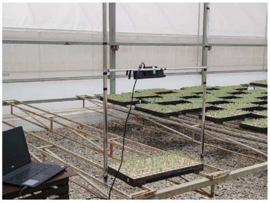
Figure 1.
ScanSeedling v1.0 Prototype showing a scan of a rigid plastic tray.
According to the National Institute of Statistics and Geography (INEGI), around three million tons of Portos tomatoes are produced in Mexico, representing approximately US$750 millon per year, the seventh-largest agricultural production in Mexico. According to Victor Villalobos, the former general of the Inter-American Institute for Cooperation in Agriculture (IICA), as stated in the National Agricultural Planning of 2017–2030, published by the ministry of the interior (SEGOB), it is necessary to increase agricultural production by at least by the year 2050 in a sustainable manner, avoiding crop losses, improving area utilization, and using less water. Finally, he proposes using technology and innovation to reduce the existing gap. On the other hand, in the same planning document, Martín Piñeiro, a special advisor to the director general of the Food and Agriculture Organization of the United Nations FAO, places Mexico as an agricultural world leader exporter.
The visual process of growth monitoring is tedious, time consuming, and error prone. The wear and tear are more noticeable in seasons when the greenhouse has a high production demand. We developed this work in six steps: (1) Concept analysis, (2) analysis of applied research, (3) design and implementation of a laboratory prototype, (4) implementation of applied research, (5) proposal and testing of a prototype in a simulated environment, and finally (6) implementation of the prototype in a natural environment. These steps allowed us to produce a low-cost and functional prototype. In addition, we propose a real-time procedure to automate the visual monitoring of the production of Portos tomatoes that achieves results in less time. Figure 2 shows the methodology proposed in six stages:
- 3D seedling scanning
- Tray point cloud extraction
- Seedling segmentation
- Morphological features extraction
- Seedling classification into four categories
- Output monitoring using a graphical user interface (GUI) that shows the classification results and provides output exporting capabilities.
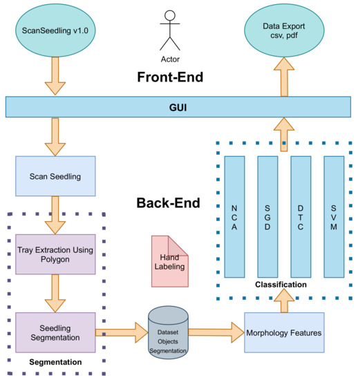
Figure 2.
The methodology is divided into six stages: 3D seedling scanning, tray point cloud extraction, seedling segmentation, height and development features extraction, seedling classification into four categories, and output monitoring.
The rest of paper is divided into four sections. Section 2 describes the related works. Section 3 describes the materials and methods in three subsections: 3D segmentation, morphological feature extraction, and seedling classification. Section 4 presents the results, Section 5 includes a discussion, and Section 6 presents the conclusions.
2. Related Works
There have been multiple approaches for seedling monitoring; Among the most used, we can find phenotyping based on laser scanning, root growth analysis, and plant growth analysis. Two-dimensional/three-dimensional data are used in controlled or uncontrolled conditions to obtain morphological characteristics spatio-temporally, with one or several viewing angles of the plant, and with one or several acquisition systems [44,45,46,47].
2.1. 2D Dynamic Measurement Systems
Nowadays, the methods using 2D data remain the basis for image analysis applied to plant growth, such as measuring and searching for characteristics. However, measurements from 2D images are often inaccurate. The work of Spalding and Miller [48] described four research trends applied to plant growth measurement: (1) Basic image analysis [49,50,51,52], (2) morphometrics [53,54], (3) kinematics [55,56], and (4) 2D versus 3D comparisons [57,58].
The works of [40,41] are carried out in natural environments. Ref. [40] detected and sprayed the plant based on volume, reducing the use of agrochemicals. In [36], the authors detected and extracted stems using stereo vision systems, arguing that stems are closely related to plant growth. In contrast, [41] calculated the seedling’s height using, stereoscopic images by converting them into disparity images to determine the depth and then obtain and segment the regions of interest. In this work, we performed the Portos tomato seedling scanning in a natural daylight environment avoiding scanning the seedling when the sun is above the sensor to avoid interference. Our prototype and the methodology proposed in this paper allows efficient and effective monitoring of the development of the Portos tomatoes seedling, one of the most expensive crops to produce in Mexico.
Currently, neural networks are used to solve many problems, including agriculture [59,60,61,62,63]. Zhang et al. [63] proposed a method to monitor the growth of lettuce in greenhouses, using images and convolutional neural networks (CNNs). They trained a model to obtain the relationship between images and growth-related traits. The authors showed that the values estimated by the CNN agree with the real measurements; they proved that this technology is a robust tool in monitoring lettuce growth in greenhouses. Neural networks’ advantage over classical methods is that they can learn from the data without manual optimization, and the segmentation can obtain highly effective results. However, we selected classical methods to reduce hardware and annotation costs. Still, however, the use of images and classical methods increase the error in monitoring any plant compared with CNNs; for this reason, we present a prototype based on 3D monitoring. We compared and optimized the methods used at each stage to reduce the need for high-cost technology.
2.2. 3D Dynamic Measurement Systems
Three-dimensional sensing methods for plant phenotyping have increased in recent years [64,65], the following works present biological applications using 3D sensing, derived traits, and different measurement techniques. The methods can be divided into six different areas or techniques: (1) Laser triangulation LT [66,67], (2) structure from motion SfM [68,69], (3) structured light SL [70,71], (4) time-of-flight ToF [72,73,74,75], (5) light field [75,76], and (6) terrestrial laser scanning TLS [77]. These techniques allow the evaluation of plant features such as seedling size, leaf width and length, volume, and development at the plant and organ level. We selected a time-of-flight (ToF) sensor for its accuracy in monitoring open environments. Unlike other sensors such as laser scanning, or structure from motion (SfM) methods, ToF has a faster processing time. Refs. [72,73] use an unmanned aerial vehicle (UAV), and [74,75] use LiDAR systems. Moreover, ToF systems are commonly inexpensive and accessible for most greenhouses in Mexico.
DiFilippo and Jouaneh [78] proposed an automatic 3D measurement system and investigated the performance of three different models of the Kinect, obtaining significant results. Our work offers a low-cost, optimized, robust, and scalable scanning prototype with real-time results. In addition, we obtained seedling growth and development to determine estimated crop yield. The low cost and fast acquisition of the Kinect make it a promising tool for field studies, especially in small stature vegetation, even though it shows limitations in daylight [34].
The works presented in [33,35,37,38,39] propose methodologies in controlled environments obtaining multiple views of the seedling and, in some cases, using rotating platforms. In the point cloud processing stage using state-of-the-art classical techniques, it is necessary to pre-process the data to obtain the 3D model of interest. The pre-processing can include stages such as background removal, outlier removal, and denoising [64]. Once the model is obtained, the processing is divided into three stages: Segmentation, feature extraction, and classification. In the first stage, according to [64], the segmentation is a critical phase in which there is no standard method that can be used because segmentation depends on the quality of the 3D data and seedling physiology. Gibbs et al. [79] propose an automatic methodology for data acquisition and retrieval of 3D plant models. The segmentation stage suggests a hybrid clustering algorithm that combines the algorithm’s principal component analysis (PCA) and modified automatic divisive hierarchical clustering (DIVFRP). Their proposal obtained better accuracy compared with K-Means, Iterative Principal Direction Divisive Partitioning (IPDDP), and spectral clustering. In our proposal, we compared and optimized K-Means and Gaussian Mixture Model GMM, and quantitatively demonstrated that GMM obtains better accuracy for plant segmentation.
The second stage entails the extraction of characteristics from the point clouds. For this task, Paturkar et al. [64] divide the approaches into three groups, including individual plant trait measurements, whole-plant measurements, and canopy-based measurements. Nguyen et al. [80] present a methodology for extracting the plant height, the number of leaves, the leaf size, and the internode distances using point clouds. First, they use Euclidean clustering to segment the plant into smaller parts. Then, they use eigenvalues to group the seedling features to extract the features. This work proposed Algorithm 1 to extract the height seedling and mean shift clustering to determine development.
| Algorithm 1 Height Seedling |
| Require: Data X where |
| Ensure: |
| procedure Projection(,) |
| if != then |
| return |
| { is minimum} |
The third stage involves classification. Guoxiang and Xiaochan [33] performed 3D point cloud reconstruction maps of the greenhouse-grown tomato plant to verify the accuracy of the extracted morphological characteristics. Furthermore, they argued that the correlation between the real values of the measurements can be calculated directly from the reconstructed 3D point cloud. In our work, we implemented, optimized, and compared five classifiers quantified using precision and recall to classify tomato seedlings into four classes: Three developmental stages and one failure.
3. Materials and Methods
This section presents a methodology for extracting, segmenting, and classifying scanned seedlings in a greenhouse. The main procedure that involves the processing of the point clouds and obtaining the morphology of the seedling to determine its growth is divided into four stages: Tray extraction of the point cloud, seedling segmentation, morphology features extraction and seedling classification; see Figure 3.
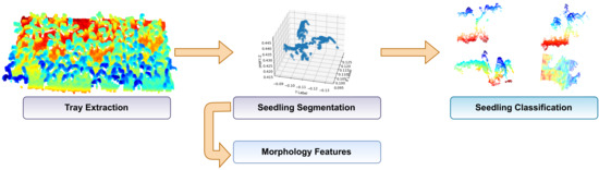
Figure 3.
Main procedure divided into four general stages. Tray extraction, seedling segmentation, features extraction: height and development, and classification of four classes.
Currently, in the central region of Mexico, seedling growth is visually monitored by trained personnel based on experience. On the 15th day of sowing the seed, the expert randomly selects of the crop trays to classify the seedling into four stages or categories: The first stage corresponds to the seedling whose growth is normal to the time of germination with average height of 6 cm as shown in Figure 4a; the second stage is the seedling whose germination occurred days after the first stage with size ranges around 4 cm in height as shown in Figure 4b; the third stage is the seedling that germinated after the second stage, and it will grow outside of the estimated harvest period; its height is less than 3 cm as shown in Figure 4c; and the fourth stage corresponds to seedlings that did not germinate.
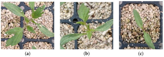
Figure 4.
Growth stages. (a) Stage 1: Seedling with normal growth on the time of germination. (b) Stage 2: Seedling whose germination occurred days after the first stage with smaller size. (c) Stage 3: Seedling that germinated after the second stage, and it will grow outside of the estimated harvest time.
The tomato seedling cultivation process is divided into five stages: (1) Seed sowing, (2) storage in germination chamber for approximately 65 h, (3) tray extended on the greenhouse, (4) germination day count 15, and (5) harvesting. Table 1 shows the five stages of the cultivation process of three different productions that we monitored for this work. Figure 5 shows the Portos tomato seedling at 15 days after sowing. The trays show irregularities because not all the seedlings have the same growth level, thus complicating monitoring and production decisions. The A1 and B2 crops differ because a new sowing technique was tried in A1. This change in sowing technique did not affect the harvest or the methodology proposed in this work.

Table 1.
Cultivation process stages. Stage 1: Seedling; stage 2: Storage in germination chamber; stage 3: Tray extended; stage 4: Germination day count; stage 5: Harvesting.
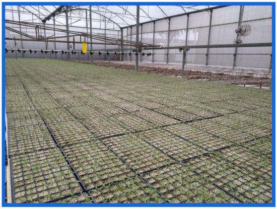
Figure 5.
Greenhouse with Portos tomato seedlings.
The monitoring or counting to determine the production is performed 15 days after sowing. In this work, we monitored of each crop; the total sample corresponds to 107 trays on three productions. Each tray had 72 cavities for a total of 7704 seedlings, of which was taken for training and for testing. We discard the outer trays for testing because they tend to have better development since they do not compete for sunlight.
Ambient temperature is vital in seedling development, so it is crucial to control the greenhouse environment. If the temperature drops outside the greenhouse, the humidity rises inside. Conversely, the moisture drops inside if the temperature rises outside the greenhouse. In central Mexico, during the summer season, the outside temperature varies on opposite poles. During the day, the temperature increases, and during the night, the temperature drops. The heat of the day allows an accelerated development of the seedling with low humidity while the humidity increases during the night. Therefore, we controlled the conditions inside the greenhouse. Figure 6 shows the temperature and humidity changes from 17 May to 24 May 2021. The green line represents the temperature, the purple line is the humidity, the horizontal line in mustard color is the high alarm, and the horizontal line in brown color is a low alarm. These climatic parameters play an important role in production.
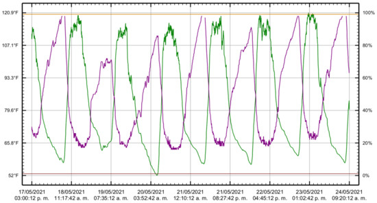
Figure 6.
Temperature and humidity changes from 17 May to 24 May 2021. The green line represents the temperature, the purple line is the humidity, the horizontal line in mustard color on top is the high alarm, and the horizontal line in brown color at the bottom represents a low alarm.
3.1. 3D Segmentation
This section describes the tray extraction and tray cavities segmentation from the rest of the image. First, we extracted the planes using the point clouds for two main reasons: To model the digitized environment in real time, separating objects with the (x,y)-plane, and reducing the computational cost and processing time. Then, we projected the point cloud to the (x,y) plane; this projection is lossless and specifies an extraction polygon with predefined coordinates to process the information of interest. The prototype design ScanSeedling v1.0 allows scanning trays in the same position. Once a tray is extracted , we applied and compared two segmentation algorithms: Gaussian Mixture Model (GMM) and K-Means. We chose these two unsupervised methods because they provide an advantage over other methods when the number of clusters is known; in this case, if we know the number of tray cavities in advance. The user provides this information from the GUI, allowing the initialization of the segmentation with n seeds, increasing the efficiency during seedling segmentation.
K-Means [81,82,83] is a technique that groups the data into K clusters. Elements that share similar features will be clustered and isolated from points that do not share similar features. To know if the data belong to the same group K-Means uses the distance between the data, and similar observations will have a smaller distance between them. We use a Euclidean distance as a measure, although there are other functions as Mahalanobis distance, Manhattan distance, Chebyshev distance, and others.
Gaussian Mixture Models (GMMs) is a probabilistic clustering model and classification method based on the probability density of the data [83,84,85]. GMMs consist of K multivariate Gaussian distributions know as mixture components, where each component k has its own parameter set where is the mean value vector and is the covariance matrix of the multivariate Gaussian. Each component of the mixture also has an associated mixing weight , where . In a graphical representation, the joint distribution is given by and the marginal distribution of x is the sum of the joint distribution over all the possible states of z. GMM is given in Equation (1).
3.2. Morphology Features
Once the seedling was segmented and the dataset created, we extracted the seedling features. This section presents the methodology of seedling height and feature extraction. The development and size of the seedling determine its stage and complement each other to achieve its classification. No matter how the seedling developed, if its height is equal to or similar to the second stage’s height, it is considered to be in the second stage.
3.2.1. Seedling Height
The agriculture process fills the tray cavities with a substrate; the seed is sown, and the agrolite is placed. Agrolite is a volcanic rock that contains water in its molecular structure; it aids decompaction, aeration, and moisture retention in seedling production. Cotyledons are the first leaves of plants; they are distinguished from the other secondary leaves of the seedling by their size, and they contain nutrients such as oil starch and can digest the albumen.
The height calculation consists of three stages: First, we normalized the points that correspond to agrolite; second, we identified the maximum height of the seedling, where the highest point commonly corresponds to the leaves because these protrude with respect to the stem; finally, we adjusted the normal to the plane of the highest point. This adjustment in all cases generated the distance in a straight line from the agrolite to the maximum height found. See Algorithm 1, where X is a point cloud, and are the minimum and maximum points on the point cloud, and receives the value of the z-axis, to obtain the projection from the highest point to the lowest point in a straight line.
3.2.2. Seedling Development
Once the height of the seedling is obtained, we segmented it, including leaves and stems. The number of leaves is unknown and varies from one seedling to another. We used the mean shift method for computing the seedling development. Mean shift is a non-supervised technique that does not need to be fed by the user. This algorithm increases the procedure’s efficiency. It can be defined as the decomposition of the sapling to analyze its homogeneous regions, which share spatial distribution and intensity characteristics. The algorithm clusters a dataset of dimension d by associating each point with the mode or peak of the probability density function. The authors of [86] present a detailed evaluation of the algorithm.
3.3. Classification
Using the morphology features identified in the previous section, we evaluated the following classifiers: Neighborhood Components Analysis (NCA), a linear model with stochastic gradient descent (SGD), a Decision Tree Classifier (DTC) or Decision Trees (DTs), a Support Vector Machine (SVM-Lineal), and a Radial Basis Function (SVM-RBF), SVM-Polynomial.
3.3.1. Neighborhood Components Analysis
This paper presents an unsupervised nearest neighbor method based on spectral clustering and manifold learning. The goal is to find a group of nearby samples that belong to an object and predict the label. The k-nearest with Euclidean distance used in this work considers the morphological data of the seedlings, which are uniformly sampled. The Neighborhood Components Analysis (NCA) is used in [87] to choose the significant features from a huge dataset. The NCA goal is to learn an optimal linear transformation matrix of size , where n is the components, and m represents the features. The goal is to learn a projection A which maximizes the samples of the probability that is correctly classified (Equation (2)).
where N is the number of samples and is the probability of the sample being correctly classified Equation (3).
is the set of points in the same class as sample i, A is a linear transformation matrix, is the softmax over Euclidean distances shown in Equation (4).
where each point j in the training set has probability of assigning its label to a point i that decays as the distance between points increases.
3.3.2. Stochastic Gradient Descent
Stochastic Gradient Descent (SGD) is used on multi-class classification problems such as text classification and natural language processing of large-scale and sparse machine learning using one versus all [88]. SGD computes the confidence score, the signed distances to the hyperplane for each classifier and chooses the class with the highest confidence. There is a set of training examples where is an arbitrary input or weight vector and , is a scalar output or the sum of squared residuals for classification. The algorithm can be divided into five steps.
- Compute the gradient of the function. The goal is to learn a linear scoring function concerning each feature. If the model has more features like to , take the partial derivative of y with respect to each of the features.
- Update the gradient function by plugging in the parameter values.
- Calculate the step sizes for each feature as
- Calculate the new parameters as
- Repeat steps 3 to 5 until the algorithm converges, i.e., the gradient is almost 0.
We used a learning rate of to avoid taking long steps down the slope.
3.3.3. Decision Tree Classifier
Decision Trees (DTs) are a non-parametric supervised learning method used for classification. The DT classifier predicts the value of the target variable using the data features through decision inferred rules [89]. It finds the features that offer the most significant entropy reduction assuming the sub-trees remain balanced. Given the feature vectors , and a label vector , a decision tree groups samples with the same labels by recursive partitions through the feature space. represents the data at node m with samples. For each candidate split consisting of a feature j and threshold and partition the data into sub-tree left (Equation (5)) and sub-tree right subsets (Equation (6)).
DTs compute a loss function to measure the quality of the splitting of the candidate node m, solving the choice of the same based on the classification Equation (7).
where minimises the impurity until allowable depth on subsets and while or . If node m obtains a classification into values , Equation (9) is applied to determine the classification criteria.
where is the proportion of class k observations in node m. If m is a terminal node, the prediction probability for this region is set to ; where k is the class and m is the node. The common impurity metrics are gini, entropy and misclassification. To avoid overfitting, we used the minimal cost-complexity pruning algorithm, parameterized by , to measure the cost-complexity of a given tree. Equation (10).
where is the number of terminal nodes in T and is defined as the total misclassification rate of the terminal nodes.
3.3.4. Suppport Vector Machine
Support Vector Machine (SVM) is a set of supervised learning methods for binary classification. Its application has been extended to multi-class classification and regression problems. In a space, a hyperplane is defined as a flat affine subspace of dimensions. In three-dimensional space, a hyperplane is a two-dimensional subspace, a conventional plane. SVM is a quadratic programming problem , separating support vectors from the rest of the data. The solver is used in a scale between and , f is the number of features, and s is the number of samples.
In this work, we evaluated a multi-class SVM as one-vs-rest classification. We evaluated three different kernels: Lineal [90], RBF exp [91] and polynomial [92], where d is specified by parameter and r by , and must be greater than 0.
4. Results
This work mimics the visual monitoring performed by a qualified expert to classify the seedling into four growth stages. We used three different crops to train and test the algorithms. This section is divided into three subsections: Segmentation, morphological features extraction, and classification.
4.1. 3D Segmentation
This section describes two stages: Tray extraction and tray cavity segmentation. When the system starts, the user provides the tray size which is used to determine the extraction polygon, and the system automatically adapts the extraction and segmentation. Figure 7a shows 72 cavity trays; Figure 7b shows the point cloud in the same tray with cavities captured using the Kinect V2.0 sensor. The color in the seedlings indicates the height, where the blue color represents the highest and red the lowest. In the point cloud shown in Figure 7c, the red-colored boxes indicate empty cavities where the seed did not germinate, the yellow-colored boxes show cavities with late seedling germination, and the green boxes show seedlings with low growth. These three boxes represent production failures. There is no way for the seedling in the red, yellow, and green boxes to achieve the seedling development categorized as stage first.
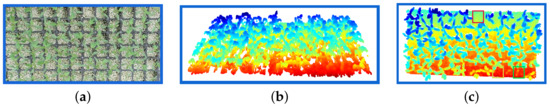
Figure 7.
Tray Extraction. (a) A cavity tray of tomato seedlings; (b) the point cloud where the color in the seedling indicates the height variation from red being the lowest to blue the highest; (c) the top-down scan of the tray shown in (a). The red, yellow, and green boxes correspond to failures.
Once we extract the trays from the point cloud, we used K-Means, and GMM methods to segment the cavities of the trays. Figure 8a shows the segmentation result using the K-Means algorithm and Figure 8b shows the segmentation performed with the GMM technique. Each segmentation is stored and processed in . Each color change represents a segmented cavity; due to graphic limitations of the programming language, in both images, the colors are repeated.
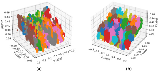
Figure 8.
Seedling segmentation. (a) The result of KMeans segmentation. (b) The segmentation with Gaussian Mixture Models.
We optimized and compared K-Means and GMM segmentation techniques; see Table 2. As ground truth, we used a hand-labeled dataset to compare both segmentation techniques. The GMM technique shows better performance for segmenting Portos tomato seedlings in 72 cavity trays; its average precision (AP) is , F1-Score , and area under the ROC curve (AUC) equals against the average precision AP , F1-Score , and AUC of of K-Means.
Table 2.
Segmentation Comparison., F1-score, average precision (AP), and Area under the ROC curve (AUC).
Once the trays were segmented, and the seedlings were extracted, we constructed the seedling dataset, labeled it, and divided it into three growth stages and failures. Figure 9 shows an example of each class of seedlings that form the training and test sets segmented with the GMM technique. Figure 9a shows a seedling in the first stage for its height and development; the red color points correspond to the agrolite, the cotidellons, the first and second true leaf. Figure 9b shows a second stage seedling. However, its height is similar to Figure 9a; its development does not correspond to a first stage seedling. Figure 9c shows the seedling in the third stage with small height; the cotyledons and the first true leaf can be observed. Figure 9d shows a cavity; the color changes correspond to agrolite and the part of the substrate where the seed did not germinate.
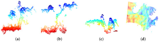
Figure 9.
Object segmentation dataset. (a–c) The first, second, and third stage seedlings, respectively. (d) An empty cavity where the seedling did not germinate.
4.2. Morphology Features
/hlDuring the first 15 days after sowing, the seedlings pass through three stages. During the first stage, they should have cotyledons and their first true leaf. Apart from the cotyledons during the second stage, their second true leaf should be emerging. Finally, in the third stage, the seedlings are about to germinate or have their cotyledons in development. In Figure 10 the agrolite is shown in red color, the leaves marked with number one correspond to cotyledons, number two are the first true leaf, and number three is the second true leaf.
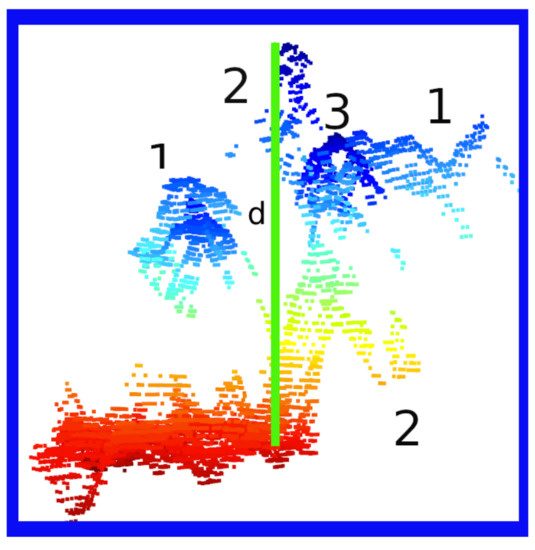
Figure 10.
Seedling Features. The red portion corresponds to the agrolite. The number one is the cotyledons, number two is the first true leaf, and number three is the second true leaf. The green line represents the normalized height of the seedling.
Algorithm 1 presented previously describes how to extract the seedling height without agrolite. First, the agrolite points are normalized; then, we obtained the highest seedling point and assigned the coordinates to the normalized points, applying a threshold of 4.15 cm to cut the seedling and eliminate any agrolite that might exist. Finally, the distance between both points defines the height of the seedling. The green vertical line represents height as shown in Figure 10. This process ensures that the agrolite and the scanned part of the tray are removed. The cavity is discarded if the outliers in the set are , counting it as a failure.
Figure 11a shows point cloud outliers resulting from the extraction, once the Portos tomato seedling is extracted. The next stage is to extract the seedling development. We used mean shift to obtain the development by segmenting each characteristic of the seedling. It segments features, where n are the segmented clusters corresponding to the leaves minus the stem. Figure 11b shows the segmentation of four leaves and stems. The points segmented with orange and red color correspond to cotyledons; in brown and green, we show the first segmented genuine leaf, and the red points represent the stem. To reduce seedlings’ over-segmentation error, we discarded distances greater than cm from the stem centroid to the centroid of each segmented leaf.
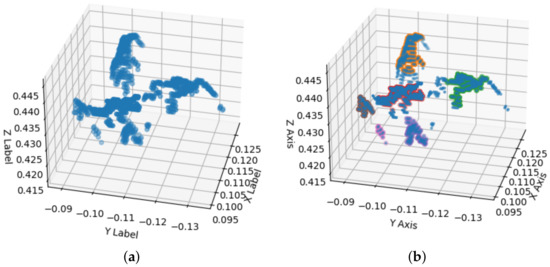
Figure 11.
Mean shift segmentation. (a) The development of a second stage seedling. (b) The segmented and counted leaves using the mean shift technique. In red and orange, we show the cotyledons, the first genuine leaf in brown and green, and the stem in pink.
We optimized the thresholds to extract the height features and seedling development at 4.15 cm and 2 cm. We obtained these values by varying the thresholds in an interval. For example, we varied the height threshold from cm to cm. For the leaf size threshold, we varied from cm to cm; in both cases, with increments of cm. We used precision and recall to quantify the optimal threshold.
4.3. Classification
The last step of our method computes the developmental stage and height features using classifiers. Then, the classifiers are used to obtain the estimated crop yield. Finally, we obtain the classification report of each classifier, the weighted mean, and the model’s accuracy.
According to greenhouse quality standards, we performed the monitoring process of the greenhouse tomato seedling on the 15th day after planting. Table 3 shows the accuracy of the six algorithms used to classify the three growth stages and the failures. Our results are compared against the expert’s accuracy, where A1, B2, and C3 are the three Portos tomato crops that were monitored. Once the crop is harvested, the expert obtains the final yield by counting the occupied cavities in the tray. The DTC classifier has the best accuracy of the six classifiers. In addition, it has the best accuracy in predicting the final yield against the expert.
Table 3.
Crop production accuracy by growth stage of each classifier against the expert’s crop production accuracy.
The model accuracy corresponds to the correct prediction count for each crop compared against the hand-labeled dataset. According to model accuracy, see Table 4, is the best classifier with correct predictions. In contrast, SGD and SVM Lineal are the worst classifiers, with an accuracy below . Our system can achieve human-level performance in predicting the final yield of Portos tomato crops.
Table 4.
Model accuracy comparison of multiple classifiers.
An error analysis showed that the expert estimates crop production with a variation of . To obtain the production, the failures are subtracted from the accuracy of the model of each classifier. The crop production or final production is obtained by a visual count of cavities containing substrate, agrolite, and, in some cases, third-stage seedlings.
Finally, Table 4 shows a summary of the model accuracy of six classifiers for the three crops analyzed. proved to be the best classifier with an average accuracy of for classifying Portos tomato seedlings into four classes. Table 5 shows results for the three test crops named A1, B2, and C3.
Table 5.
Results for the three test crops named A1, B2, C3 and a weighted average.
We used precision and recall to evaluate the performance of the classification algorithms. Class 0 represents the failures, class 1 corresponds to the third stage, class 2 is the second stage, and class 3 represents the first stage. Figure 12 shows the precision for each class and the micro-average precision-recall of the four classes. Visually we can determine which algorithm performs best. The best performing algorithms for classifying the three stages and seedling failures are observed close to the [1,1] point of the quadrant, starting at the [0,1] point and ending at the [1,0] point. In contrast, the worst ranking results are far from the [1,1] point and, in some cases, often end at the origin. The yellow color represents the micro-average precision-recall of the four classes. The blue curve represents class 0, cyan corresponds to class 1, orange is class 2, and purple is class 3. DTC obtains the best micro-average precision-recall with area . At the same time, the worst micro-average precision-recall is from GSD with area = .
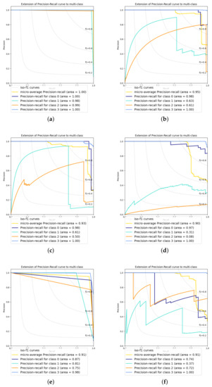
Figure 12.
Precision and recall for the six classifiers (a) DTC, (b) SVM Poly, (c) SVM RBF, (d) SGD, (e) SVM Linear, and (f) NCA. The figures show the area of the curve for each growth stage, faults, and the model’s micro-average.
On the other hand, the sensor viewing angle and trays are parallel during the seedling scanning. This angle favors the correct extraction of height and seedling development features. However, this viewing angle generates occlusion of most seedling stems, especially the first stage seedling. Algorithm 1 is used to obtain the height effectively.
5. Discussion
This prototype aims to test the correct functioning of the Kinect in a natural greenhouse environment, detect the ideal parameters to position the Kinect in the three axes , and improve the results of the expert to determine the growth and development of the Portos tomato seedling. It is important to remember that the monitoring of the seedling is performed in one single stage, on the 15th day after planting. Therefore, the monitoring objectives can be divided into two phases: The first objective is to decide agrochemical application and water use, and the second objective is to predict final crop production.
In this project, we showed that it is possible to scan and monitor the seedlings during daylight using a Kinect sensor in natural greenhouse conditions. After testing the Kinect sensor, we found four situations where the Kinect reduces its acquisition capabilities:
- When the Kinect is facing the sun.
- When the sunlight is covering the sensor.
- When the scanning zone includes light and shadow.
- When overgrown plants occlude the others.
Considering the complexity of agricultural ecosystems, the methodology proposed in this work to extract the morphology in Portos tomato seedlings is compelling. The expert’s knowledge allows us to evaluate the proposed algorithms on three different Portos tomato crops. Figure 13 shows the normal distribution of Portos tomato seedling height test. It is shown that the measurement values were linearly related to the manual measurement values. Figure 13a shows culture A1, Figure 13b presents culture B2, and finally, in Figure 13c, we can see culture C3. The relative weighted average error at day 15 monitoring in three crops on our proposal against expert results is .
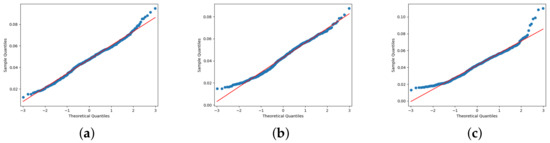
Figure 13.
Test of Normal Distribution. Data distribution and fitting results for Portos tomato seedling height. The figures show crops A1, B2, and C3, respectively. (a) shows culture A1, (b) presents culture B2, and finally, in (c), we can see culture C3.
The expert’s final production weighted average error was and our system weighted average error was . Therefore, it is quantitatively demonstrated that our proposal reduced the error in predicting the final production of Portos tomatoes. The time to scan the seedling is about 0.2 s, the time to extract the tray from the point cloud is about s, the time to segment a tray of 72 cavities is s, and the total time to obtain height and development of the tomato seedling is s.
The labeling of the data used to train and test the algorithms was performed using software developed by the authors. Our system automatically scans the seedling, then extracts the tray using the polygon given by the user, then it segments the seedling using the Gaussian Mixture Models (GMMs) and extracts the seedling morphology, development, and height. Finally, it classifies the seedling into four categories using a Decision Tree Classifier (DTC). The GMM segmentation, DTC classification algorithms, and GUI are mounted in a local server. The server saves historical data of crop monitoring. Once the production monitoring process is finished, the GUI gives the end-user the option to download the monitoring report as a .csv or .pdf file.
We used python language to implement, optimize, and compare the algorithms. The Kinect is configured using the Robot Operating System (ROS) embedded into the python GUI. We used a mid-range laptop with a 7th gen i3, 4 cores, and 8 GB of RAM.
The use of the depth sensor in an outdoor environment required its calibration [93,94]. Therefore, we performed the sensor calibration in an indoor environment controlling the illumination received by the pattern, mainly in the back of the pattern and the front of the Kinect sensor. We used a standard 3 cm calibration pattern and collected images of the pattern at m and m distance from the sensor. As a result, we got a re-projection error for color, depth, and both concerning , , pixels, respectively.
The innovation of any technology development project is measured using the TRL levels proposed by the National Aeronautics and Space Administration (NASA). The project presented here entails six stages, described in the introduction section. These stages allow positioning the technological development in nine TRL maturity levels. Our prototype complies with the legal standards of Mexican agronomy and has been tested in a natural greenhouse environment; therefore, the level that corresponds to this development is the TRL-5 maturity level. The prototype and GUI (front end) and computational algorithms (back end) work accurately without modifying greenhouse conditions.
According to the manufacturer’s specifications, the seed used in the three crops was labeled in March 2020 with germination. We labeled the datasets by hand with the help of greenhouse experts. Our method optimized the segmentation and classification for the specific task achieving a segmentation with an average precision of , and a classification accuracy of .
We compare our work with those of Yang et al. [95] and Ma et al. [96] as they are the most similar to our research. In [95] is described the difficulty of finding a quantitative comparison criterion because the approaches focus on different tasks, while in [95,96], they scanned the seedling, placing the sensor over the seedling; [96] performed the scans outdoors, while in [95] and our proposed approach they were performed inside a greenhouse under natural conditions. Our work has three main differences concerning [95,96], namely the background and/or tray extraction, the seedling segmentation, and the morphology extraction. In [96] the authors extract the bottom according to a depth threshold and segment the seedling; the results are inaccurate if the crop is very dense. In [95], they propose to use FPFH to describe each point and employ K-means to cluster the bottom and crop points, extracting the bottom and the seedling tray. In our proposal, the user feeds the GUI with the type of tray to be processed, the point cloud is projected to the axes without losing information, and a polygon is used for extracting the tray. This process reduces the computational cost processes.
The segmentation stage in [96] knows in advance the sizes of the pots and crops; in [95], the authors use the VCCS and LCCP-based algorithms, while we propose an automatic segmentation comparing the performance of K-means and GMM. The last comparison is according to the morphology extraction. In [96], the authors include the color indices, and [95] included leaf area and canopy breadth. Our methodology extracts seedling development using mean shift, by stem count and the number of first true leaves and cotyledons. Finally, the height and development information allows us to classify the seedling according to its growth stage. In summary, our approach is based on robust algorithms and relies on a single pre-set parameter to extract the tray. This is because greenhouses in Mexico use trays with different characteristics such as height, length, width, number of cavities, and shape. Hence, the proposed procedure works for any tray type and makes it a general approach.
6. Conclusions
Seedling monitoring was carried out in central Mexico in late spring and early summer. These tests do not need repeating at other times of the year due to the internal conditions of the greenhouse. The methodology proposed in this work offers a new approach to seedling measurement in greenhouses. Our system uses different algorithms for each stage: ROS for scanning as shown in Figure 1; tray extraction using the proposed method and seedling segmentation using the GMM method as described in Section 3.1; morphology extraction using Algorithm 1 and seedling classification using the DTC algorithm, as shown in Section 3.3. Our results reveal that the optimized algorithms and the comparison allow us to obtain a predictive model for the harvest with less error than specialized personnel and in less time. Our system is affordable and easy to transport and install without modifying the greenhouse conditions.
Future works intend to propose a mechatronic system that allows scanning the totality of the crop trays. A remaining challenge in this proposal is the computational time that is considerably increased by using a method such as mean shift to segment each cotyledon, leaf, and stem. We plan to detect the development at a significantly shorter computational time. In addition, the algorithms and GUI will be scaled and determine the production of multiple tomato varieties and seedling types such as corn, carrots, onions, or watermelon, to name a few.
Author Contributions
A.R.-P. was involved in methodology, software developed, prototype implementation and writing original draft. J.-J.G.-B. was involved in prototype implementation, data acquisition and writing original draft. F.-J.O.-R. was involved in data pre-processing and hand labeling. D.-M.C.-E. and E.-A.G.-B. was involved in prototype desing and software validation. All authors have read and agreed to the published version of the manuscript.
Funding
This research received no funding.
Institutional Review Board Statement
Not applicable.
Informed Consent Statement
Not applicable.
Data Availability Statement
Not applicable.
Acknowledgments
To the CONACyT, for supporting project number 669. Also want to thank Greenhouse Apatzeo, especially to enginner Jorge Montes and collaborators.
Conflicts of Interest
The authors declare that they have no conflict of interes.
Abbreviations
The following abbreviations are used in this manuscript:
| ROI | Region of Interest |
| LT | Laser Triangulation |
| SfM | Structure from Motion |
| SL | Structure Light |
| ToF | Time-of-Flight |
| LF | Light Field |
| TLS | Terrestrial Laser Scanning |
| INEGI | National Institute of Statistics and Geography |
| SEGOB | Ministry of the Interior |
| IICA | Institute for Cooperation in Agriculture |
| FAO | Food and Agriculture Organization of the United Nations |
| 3D | three-dimensional |
| 2D | two-dimensional |
| UAV | Unmanned Aerial Vehicle |
| LiDAR | Light Detection And Ranging |
| PCA | Principal Component Analysis |
| DIVFRP | Automatic Divisive Hierarchical Clustering |
| IPDDP | Iterative Principal Direction Divisive Partitioning |
| GMM | Gaussian Mixture Model |
| DTC | Decision Tree Classifier |
| GUI | Graphical User Interface |
| NCA | Neighborhood Components Analysis |
| SGD | Stochastic Gradient Descent |
| OVA | One Versus All |
| DTC | Decision Tree Classifier |
| DTs | Decision Trees |
| QPp | Quadratic Programming Problem |
| SVM | Support Vector Machine |
| RBF | Radial Basis Function |
| Germ. | Germination |
| A1 | Crop Germ. May 20 |
| B2 | Crop Germ. May 20 |
| C3 | Crop Germ. Jun 19 |
| AUC | Area Under Curve |
| AP | Average Precision |
| NASA | National Aeronautics and Space Administration |
| VCCS | Voxel Cloud Connectivity Segmentation |
| LCCP-based | Locally Convex Connected Patches |
| ROS | Robot Operating System |
References
- Abdelazeem, M.; Elamin, A.; Afifi, A.; El-Rabbany, A. Multi-sensor point cloud data fusion for precise 3D mapping. Egypt. J. Remote Sens. Space Sci. 2021, 24, 835–844. [Google Scholar] [CrossRef]
- Štrbac, M.; Marković, M.; Popović, D.B. Kinect in neurorehabilitation: Computer vision system for real time hand and object detection and distance estimation. In Proceedings of the 11th Symposium on Neural Network Applications in Electrical Engineering, Belgrade, Serbia, 20–22 September 2012; pp. 127–132. [Google Scholar] [CrossRef]
- Ballit, A.; Mougharbel, I.; Ghaziri, H.; Dao, T.T. Visual Sensor Fusion with Error Compensation Strategy Toward a Rapid and Low-Cost 3D Scanning System for the Lower Residual Limb. IEEE Sens. J. 2020, 20, 15043–15052. [Google Scholar] [CrossRef]
- Kazuki, K.; Takashi, K.; Keiichiro, K.; Shoji, K. Transmission of correct gaze direction in video conferencing using screen-embedded cameras. Multimed. Tools Appl. 2021, 80, 31509–31526. [Google Scholar] [CrossRef]
- Pal, D.H.; Kakade, S.M. Dynamic hand gesture recognition using Kinect sensor. In Proceedings of the International Conference on Global Trends in Signal Processing, Information Computing and Communication (ICGTSPICC), Jalgaon, India, 22–24 December 2016; pp. 448–453. [Google Scholar] [CrossRef]
- Hoque, S.M.A.; Haq, M.S.; Hasanuzzaman, M. Computer Vision Based Gesture Recognition for Desktop Object Manipulation. In Proceedings of the International Conference on Innovation in Engineering and Technology (ICIET), Dhaka, Bangladesh, 27–28 December 2018; pp. 1–6. [Google Scholar] [CrossRef]
- Chikkanna, M.; Guddeti, R.M.R. Kinect based real-time gesture spotting using HCRF. In Proceedings of the International Conference on Advances in Computing, Communications and Informatics (ICACCI), Mysore, India, 22–25 August 2013; pp. 925–928. [Google Scholar] [CrossRef]
- Stanev, D.; Moustakas, K. Virtual Human Behavioural Profile Extraction Using Kinect Based Motion Tracking. In Proceedings of the International Conference on Cyberworlds, Cantabria, Spain, 6–8 October 2014; pp. 411–414. [Google Scholar] [CrossRef]
- Jagdish, R.; Mona, C.; Ankit, C. 3D Gesture based Real-time Object Selection and Recognition. Pattern Recognit. Lett. 2017, 115, 14–19. [Google Scholar] [CrossRef]
- Lun, R.; Zhao, W. A Survey of Applications and Human Motion Recognition with Microsoft Kinect. Int. J. Pattern Recognit. Artif. Intell. 2015, 29, 1555008. [Google Scholar] [CrossRef] [Green Version]
- Owens, J. Object Detection Using the Kinect; Army Research Laboratory: Aberdeen Proving Ground, MD, USA, 2012. [Google Scholar]
- Le, V.; Vu, H.; Nguyen, T.T.; Le, T.; Tran, T.; Vlaminck, M.; Philips, W.; Veelaert, P. 3D Object Finding Using Geometrical Constraints on Depth Images. In Proceedings of the Seventh International Conference on Knowledge and Systems Engineering (KSE), Ho Chi Minh City, Vietnam, 8–10 October 2015; pp. 389–394. [Google Scholar] [CrossRef]
- Antonio, C.; David, F.L.; Montemayor, A.S.; José, P.J.; Luisa, D.M. Abandoned Object Detection on Controlled Scenes Using Kinect. In Natural and Artificial Computation in Engineering and Medical Applications; Springer: Berlin/Heidelberg, Germany, 2013; pp. 169–178. [Google Scholar]
- Afanasyev, I.; Biasi, N.; Baglivo, L.; Cecco, M.D. 3D Object Localization using Superquadric Models with a Kinect Sensor. 2011. Available online: https://www.semanticscholar.org/paper/3D-Object-Localization-using-Superquadric-Models-a-Afanasyev-Nicolo’Biasi/d14f9860902a505c2e36594601186f10be2eafaf (accessed on 15 January 2022).
- Cheong, H.; Kim, E.; Park, S. Indoor Global Localization Using Depth-Guided Photometric Edge Descriptor for Mobile Robot Navigation. IEEE Sens. J. 2019, 19, 10837–10847. [Google Scholar] [CrossRef]
- Tsoli, A.; Argyros, A.A. Tracking Deformable Surfaces That Undergo Topological Changes Using an RGB-D Camera. In Proceedings of the Fourth International Conference on 3D Vision (3DV), Stanford, CA, USA, 25–28 October 2016; pp. 333–341. [Google Scholar] [CrossRef]
- Andrés, D.T.; Lina, P.P.; Pedro, P.R.; Eduardo, C.B. Dense tracking, mapping and scene labeling using a depth camera. In Revista Facultad de Ingeniería Universidad de Antioquia. 2018, pp. 54–69. Available online: https://revistas.udea.edu.co/index.php/ingenieria/article/view/328187 (accessed on 15 January 2022).
- Jung, J.W.; Jeon, J.W. Control of the manipulator position with the Kinect sensor. In Proceedings of the IECON—43rd Annual Conference of the IEEE Industrial Electronics Society, Beijing, China, 29 October–1 November 2017; pp. 2991–2996. [Google Scholar] [CrossRef]
- Afthoni, R.; Rizal, A.; Susanto, E. Proportional derivative control based robot arm system using Microsoft Kinect. In Proceedings of the International Conference on Robotics, Biomimetics, Intelligent Computational Systems, Jogjakarta, Indonesia, 25–27 November 2013; pp. 24–29. [Google Scholar] [CrossRef]
- Gonzalez, P.; Cheng, M.; Kuo, W. Vision-based robotic system for polyhedral object grasping using Kinect sensor. In Proceedings of the International Automatic Control Conference (CACS), Taichung, Taiwan, 9–11 November 2016; pp. 71–76. [Google Scholar] [CrossRef]
- Carvalho, C.A.T. Development of Robotic Arm Control System Using Computational Vision. IEEE Lat. Am. Trans. 2019, 17, 1259–1267. [Google Scholar]
- Junemann, M. 3D Object Localization using Superquadric Models with a Kinect Sensor Object Detection and Recognition with Microsoft Kinect. 2012. Available online: https://apps.dtic.mil/sti/pdfs/ADA564736.pdf (accessed on 15 January 2022).
- Shin, D.; Ho, Y. Implementation of 3D object reconstruction using a pair of Kinect cameras. In Proceedings of the Signal and Information Processing Association Annual Summit and Conference (APSIPA), 2014 Asia-Pacific, Chiang Mai, Thailand, 9–12 December 2014; pp. 1–4. [Google Scholar] [CrossRef]
- Woodard, W.; Sukittanon, S. Interactive virtual building walkthrough using Oculus Rift and Microsoft Kinect. In Proceedings of the SoutheastCon 2015, Fort Lauderdale, FL, USA, 9–12 April 2015; pp. 1–3. [Google Scholar] [CrossRef]
- Peter, H.; Michael, K.; Evan, H.; Xiaofeng, R.; Dieter, F. RGB-D Mapping: Using Kinect-Style Depth Cameras for Dense 3D Modeling of Indoor Environments. Int. J. Robot. Res.-IJRR 2012, 31, 647–663. [Google Scholar] [CrossRef] [Green Version]
- Camplani, M.; Mantecón, T.; Salgado, L. Depth-Color Fusion Strategy for 3-D Scene Modeling With Kinect. IEEE Trans. Cybern. 2013, 43, 1560–1571. [Google Scholar] [CrossRef]
- Majdi, A.; Bakkay, M.C.; Zagrouba, E. 3D modeling of indoor environments using Kinect sensor. In Proceedings of the IEEE Second International Conference on Image Information Processing (ICIIP-2013), Shimla, India, 9–11 December 2013; pp. 67–72. [Google Scholar] [CrossRef]
- Jaiswal, M.; Xie, J.; Sun, M. 3D object modeling with a Kinect camera. In Proceedings of the Signal and Information Processing Association Annual Summit and Conference (APSIPA), Asia-Pacific, Chiang Mai, Thailand, 9–12 December 2014; pp. 1–5. [Google Scholar] [CrossRef]
- Xu, H.; Wang, X.; Shi, L. Fast 3D-Object Modeling with Kinect and Rotation Platform. In Proceedings of the Third International Conference on Robot, Vision and Signal Processing (RVSP), Kaohsiung, Taiwan, 18–20 November 2015; pp. 43–46. [Google Scholar] [CrossRef]
- Procházka, A.; Vysata, O.; Scätz, M.; Charvátova, H.; Paz Suarez Araujo, C.; Geman, O.; Marik, V. Video processing and 3D modelling of chest movement using MS Kinect depth sensor. In Proceedings of the International Workshop on Computational Intelligence for Multimedia Understanding (IWCIM), Reggio Calabria, Italy, 27–28 October 2016; pp. 1–5. [Google Scholar] [CrossRef]
- Shen, B.; Yin, F.; Chou, W. A 3D Modeling Method of Indoor Objects Using Kinect Sensor. In Proceedings of the 10th International Symposium on Computational Intelligence and Design (ISCID), Hangzhou, China, 9–10 December 2017; Volume 1, pp. 64–68. [Google Scholar] [CrossRef]
- Ding, J.; Chen, J.; Zhou, A.; Chen, Z. 3D Modeling of the Rotationally Symmetric Objects Using Kinect. In Proceedings of the IEEE 4th International Conference on Image, Vision and Computing (ICIVC), Xiamen, China, 5–7 July 2019; pp. 685–689. [Google Scholar] [CrossRef]
- Guoxiang, S.; Xiaochan, W. Three-Dimensional Point Cloud Reconstruction and Morphology Measurement Method for Greenhouse Plants Based on the Kinect Sensor Self-Calibration. Agronomy 2019, 9, 596. [Google Scholar] [CrossRef] [Green Version]
- Azzari, G.; Goulden, M.L.; Rusu, R.B. Rapid Characterization of Vegetation Structure with a Microsoft Kinect Sensor. Sensors 2013, 13, 2384–2398. [Google Scholar] [CrossRef] [Green Version]
- Yang, H.; Le, W.; Lirong, X.; Qian, W.; Huanyu, J. Automatic Non-Destructive Growth Measurement of Leafy Vegetables Based on Kinect. Sensors 2018, 18, 806. [Google Scholar] [CrossRef] [Green Version]
- Fu, D.; Xu, L.; Li, D.; Xin, L. Automatic detection and segmentation of stems of potted tomato plant using Kinect. In Proceedings of the Sixth International Conference on Digital Image Processing (ICDIP), Athens, Greece, 5–6 April 2014; Falco, C.M., Chang, C.C., Jiang, X., Eds.; International Society for Optics and Photonics, SPIE: Bellingham, WA, USA, 2014; Volume 9159, pp. 18–22. [Google Scholar] [CrossRef]
- Nasir, A.K.; Taj, M.; Khan, M.F. Evaluation of Microsoft Kinect Sensor for Plant Health Monitoring. In Proceedings of the 5th IFAC Conference on Sensing, Control and Automation Technologies for Agriculture AGRICONTROL, Seattle, WA, USA, 14–17 August 2016; Volume 49, pp. 221–225. [Google Scholar] [CrossRef]
- Mengzhu, X. Surface Reconstruction and Parameter Measurement of Plant Based on Structured Light Point Cloud. 2021. Available online: https://caod.oriprobe.com/articles/61489684/Surface_reconstruction_and_parameter_measurement_o.htm (accessed on 15 January 2022).
- Hua, S.; Xu, M.; Xu, Z.; Ye, H.; Zhou, C.Q. Kinect-Based Real-Time Acquisition Algorithm of Crop Growth Depth Images. Math. Probl. Eng. 2012, 2021, 221–225. [Google Scholar] [CrossRef]
- Hojat, H.; Jafar, M.; Keyvan, A.V.; Mohsen, S.; Gholamreza, C. Design, manufacture and evaluation of automatic spraying mechanism In order to increase productivity. J. Agric. Eng. Soil Sci. Agric. Mech. (Sci. J. Agric.) 2021, 44. [Google Scholar] [CrossRef]
- Kim, W.S.; Lee, D.H.; Kim, Y.J.; Kim, T.; Lee, W.S.; Choi, C.H. Stereo-vision-based crop height estimation for agricultural robots. Comput. Electron. Agric. 2021, 181, 105937. [Google Scholar] [CrossRef]
- Tian, G.; Feiyu, Z.; Puneet, P.; Jaspreet, S.; Akrofi, D.H.; Jianxin, S.; Yu, P.; Paul, S.; Harkamal, W.; Hongfeng, Y. Novel 3D Imaging Systems for High-Throughput Phenotyping of Plants. Remote Sens. 2021, 13, 2113. [Google Scholar] [CrossRef]
- Dobrota, C.T.; Carpa, R.; Butiuc-Keul, A. Analysis of designs used in monitoring crop growth based on remote sensing methods. Turk. J. Agric. For. 2021, 45, 730–742. [Google Scholar] [CrossRef]
- Alkan, A.; Abdullah, M.; Abdulah, H.; Assaf, M.; Zhou, H. A smart agricultural application: Automated Detection of Diseases in Vine Leaves Using Hybrid Deep Learning. Turk. J. Agric. For. 2021, 45, 717–729. [Google Scholar] [CrossRef]
- Dornbusch, T.; Séverine, L.; Dmitry, K.; Arnaud, F.; Robin, L.; Ioannis, X.; Fankhauser, C. Measuring the diurnal pattern of leaf hyponasty and growth in Arabidopsis – a novel phenotyping approach using laser scanning. Funct. Plant Biol. 2012, 39, 860–869. [Google Scholar] [CrossRef] [Green Version]
- Paramita, B.; Anupam, P. A new tool for analysis of root growth in the spatio-temporal continuum. New Phytol. 2012, 195, 264–274. [Google Scholar] [CrossRef]
- Wahyu, S.; Rudiati, M.; Balza, A. Development of Plant Growth Monitoring System Using Image Processing Techniques Based on Multiple Images; Springer: Cham, Switzerland, 2017; pp. 647–653. [Google Scholar] [CrossRef]
- Spalding, E.P.; Miller, N.D. Image analysis is driving a renaissance in growth measurement. Curr. Opin. Plant Biol. 2013, 16, 100–104. [Google Scholar] [CrossRef] [PubMed] [Green Version]
- Li, C.; Adhikari, R.; Yao, Y.; Miller, A.G.; Kalbaugh, K.; Li, D.; Nemali, K. Measuring plant growth characteristics using smartphone based image analysis technique in controlled environment agriculture. Comput. Electron. Agric. 2020, 168, 105–123. [Google Scholar] [CrossRef]
- John, C. A Computational Approach to Edge Detection. IEEE Trans. Pattern Anal. Mach. Intell. 1986, PAMI-8, 679–698. [Google Scholar] [CrossRef]
- Harris, C.G.; Stephens, M. A Combined Corner and Edge Detector. In Proceedings of the Alvey Vision Conference, Manchester, UK, 31 August–2 September 1988. [Google Scholar]
- Nobuyuki, O. AA Threshold Selection Method from Gray-Level Histograms. IEEE Trans. Syst. Man Cybern. 1979, 9, 62–66. [Google Scholar] [CrossRef] [Green Version]
- Guamba, J.C.C.; Corredor, D.; Galárraga, C.; Herdoiza, J.P.; Santillán, M.; Segovia-Salcedo, M.C. Geometry morphometrics of plant structures as a phenotypic tool to differentiate Polylepis incana Kunth. and Polylepis racemosa Ruiz & Pav. reforested jointly in Ecuador. Neotrop. Biodivers. 2021, 7, 121–134. [Google Scholar] [CrossRef]
- Benjamin, C.; Steve, K.; Joanne, C. Automated analysis of hypocotyl growth dynamics during shade avoidance in Arabidopsis. Plant J. Cell Mol. Biol. 2010, 65, 991–1000. [Google Scholar] [CrossRef] [Green Version]
- Bertels, J.; Beemster, G.T. leafkin—An R package for automated kinematic data analysis of monocot leaves. Quant. Plant Biol. 2020, 1, e2. [Google Scholar] [CrossRef]
- Nelson, A.; Evans, M. Analysis of growth patterns during gravitropic curvature in roots ofZea mays by use of a computer-based video digitizer. J. Plant Growth Regul. 2005, 5, 73–83. [Google Scholar] [CrossRef]
- Smith, L.N.; Zhang, W.; Hansen, M.F.; Hales, I.J.; Smith, M.L. Innovative 3D and 2D machine vision methods for analysis of plants and crops in the field. Comput. Ind. 2018, 97, 122–131. [Google Scholar] [CrossRef]
- Taras, G.; Yuriy, M.; Alexander, B.; Brad, M.; Olga, S.; Charles, P.; Christopher, T.; Anjali, I.P.; Paul, Z.; Suqin, F.; et al. GiA Roots: Software for the high throughput analysis of plant root system architecture. BMC Plant Biol. 2012, 12, 116. [Google Scholar] [CrossRef] [Green Version]
- Boogaard, F.P.; Rongen, K.S.; Kootstra, G.W. Robust node detection and tracking in fruit-vegetable crops using deep learning and multi-view imaging. Biosyst. Eng. 2020, 192, 117–132. [Google Scholar] [CrossRef]
- Du, J.; Lu, X.; Fan, J.; Qin, Y.; Yang, X.; Guo, X. Image-Based High-Throughput Detection and Phenotype Evaluation Method for Multiple Lettuce Varieties. Front. Plant Sci. 2020, 11, 3386. [Google Scholar] [CrossRef] [PubMed]
- Ahsan, M.; Eshkabilov, S.; Cemek, B.; Küçüktopcu, E.; Lee, C.W.; Simsek, H. Deep Learning Models to Determine Nutrient Concentration in Hydroponically Grown Lettuce Cultivars. Sustainability 2022, 14, 416. [Google Scholar] [CrossRef]
- Chang, S.; Lee, U.; Hong, M.J.; Jo, Y.D.; Kim, J.B. Lettuce Growth Pattern Analysis Using U-Net Pre-Trained with Arabidopsis. Agriculture 2021, 11, 890. [Google Scholar] [CrossRef]
- Zhang, L.; Xu, Z.; Xu, D.; Ma, J.; Chen, Y.; Fu, Z. Growth monitoring of greenhouse lettuce based on a convolutional neural network. Hortic. Res. 2020, 7, 124. [Google Scholar] [CrossRef]
- Paturkar, A.; Sen Gupta, G.; Bailey, D. Making Use of 3D Models for Plant Physiognomic Analysis: A Review. Remote Sens. 2021, 13, 2232. [Google Scholar] [CrossRef]
- Stefan, P. Measuring crops in 3D: Using geometry for plant phenotyping. Plant Methods 2019, 15, 1–13. [Google Scholar]
- Virlet, N.; Sabermanesh, K.; Sadeghi-Tehran, P.; Hawkesford, M.J. Field Scanalyzer: An automated robotic field phenotyping platform for detailed crop monitoring. Funct Plant Biol. 2016, 1, 143–153. [Google Scholar] [CrossRef] [Green Version]
- Jan, D.; Heiner, K. High-Precision Surface Inspection: Uncertainty Evaluation within an Accuracy Range of 15 μm with Triangulation-based Laser Line Scanners. J. Appl. Geod. 2014, 8, 109–118. [Google Scholar] [CrossRef]
- Cao, M.; Jia, W.; Lv, Z.; Li, Y.; Xie, W.; Zheng, L.; Liu, X. Fast and robust feature tracking for 3D reconstruction. Opt. Laser Technol. 2019, 110, 120–128. [Google Scholar] [CrossRef]
- Moeckel, T.; Dayananda, S.; Nidamanuri, R.R.; Nautiyal, S.; Hanumaiah, N.; Buerkert, A.; Wachendorf, M. Estimation of Vegetable Crop Parameter by Multi-temporal UAV-Borne Images. Remote Sens. 2018, 10, 805. [Google Scholar] [CrossRef] [Green Version]
- Zhang, S. High-speed 3D shape measurement with structured light methods: A review. Opt. Lasers Eng. 2018, 106, 119–131. [Google Scholar] [CrossRef]
- Li, L.; Schemenauer, N.; Peng, X.; Zeng, Y.; Gu, P. A reverse engineering system for rapid manufacturing of complex objects. Robot. Comput.-Integr. Manuf. 2002, 18, 53–67. [Google Scholar] [CrossRef]
- Luo, S.; Liu, W.; Zhang, Y.; Wang, C.; Xi, X.; Nie, S.; Ma, D.; Lin, Y.; Zhou, G. Maize and soybean heights estimation from unmanned aerial vehicle (UAV) LiDAR data. Comput. Electron. Agric. 2021, 182, 106005. [Google Scholar] [CrossRef]
- Estornell, J.; Hadas, E.; Martí, J.; López-Cortés, I. Tree extraction and estimation of walnut structure parameters using airborne LiDAR data. Int. J. Appl. Earth Obs. Geoinf. 2021, 96, 102273. [Google Scholar] [CrossRef]
- Qiu, Q.; Sun, N.; Bai, H.; Wang, N.; Fan, Z.; Wang, Y.; Meng, Z.; Li, B.; Cong, Y. Field-Based High-Throughput Phenotyping for Maize Plant Using 3D LiDAR Point Cloud Generated with a “Phenomobile”. Front. Plant Sci. 2019, 10, 554. [Google Scholar] [CrossRef] [Green Version]
- Thapa, S.; Zhu, F.; Walia, H.; Yu, H.; Ge, Y. A Novel LiDAR-Based Instrument for High-Throughput, 3D Measurement of Morphological Traits in Maize and Sorghum. Sensors 2018, 18, 1187. [Google Scholar] [CrossRef] [Green Version]
- Paturkar, A.; Gupta, G.S.; Bailey, D. 3D Reconstruction of Plants Under Outdoor Conditions Using Image-Based Computer Vision. Recent Trends in Image Processing and Pattern Recognition; Santosh, K.C., Hegadi, R.S., Eds.; Springer: Singapore, 2019; pp. 284–297. [Google Scholar]
- Disney, M. Terrestrial LiDAR: A 3D revolution in how we look at trees. New Phytol. 2018, 222, 1736–1741. [Google Scholar] [CrossRef] [Green Version]
- DiFilippo, N.M.; Jouaneh, M.K. Characterization of Different Microsoft Kinect Sensor Models. IEEE Sens. J. 2015, 15, 4554–4564. [Google Scholar] [CrossRef]
- Gibbs, J.A.; Pound, M.P.; French, A.P.; Wells, D.M.; Murchie, E.H.; Pridmore, T.P. Active Vision and Surface Reconstruction for 3D Plant Shoot Modelling. IEEE/ACM Trans. Comput. Biol. Bioinform. 2020, 17, 1907–1917. [Google Scholar] [CrossRef]
- Nguyen, T.; Slaughter, D.; Max, N.; Maloof, J.; Sinha, N. Structured Light-Based 3D Reconstruction System for Plants. Sensors 2015, 15, 18587–18612. [Google Scholar] [CrossRef] [PubMed] [Green Version]
- Sankaran, K.; Vasudevan, N.; Nagarajan, V. Plant Disease Detection and Recognition using K means Clustering. In Proceedings of the International Conference on Communication and Signal Processing (ICCSP), Chennai, India, 28–30 July 2020; pp. 1406–1409. [Google Scholar] [CrossRef]
- Rani, F.P.; Kumar, S.; Fred, A.L.; Dyson, C.; Suresh, V.; Jeba, P. K-means Clustering and SVM for Plant Leaf Disease Detection and Classification. In Proceedings of the International Conference on Recent Advances in Energy-efficient Computing and Communication (ICRAECC), Nagercoil, India, 7–8 March 2019; pp. 1–4. [Google Scholar] [CrossRef]
- Andri, M. Statistical Analysis of Microarray Data Clustering using NMF, Spectral Clustering, Kmeans, and GMM. IEEE/ACM Trans. Comput. Biol. Bioinform. 2020. [Google Scholar] [CrossRef]
- Chaudhury, A.; Godin, C. Skeletonization of Plant Point Cloud Data Using Stochastic Optimization Framework. Front. Plant Sci. 2020, 11, 773. [Google Scholar] [CrossRef] [PubMed]
- Zhou, F.; Li, M.; Yin, L.; Yuan, X. Image segmentation algorithm of Gaussian mixture model based on map/reduce. In Proceedings of the Chinese Automation Congress (CAC), Jinan, China, 20–22 October 2017; pp. 1520–1525. [Google Scholar] [CrossRef]
- Xiao, W.; Zaforemska, A.; Smigaj, M.; Wang, Y.; Gaulton, R. Mean Shift Segmentation Assessment for Individual Forest Tree Delineation from Airborne Lidar Data. Remote Sens. 2019, 11, 1263. [Google Scholar] [CrossRef] [Green Version]
- Mohammed Hashim, B.A.; Amutha, R. Machine Learning-based Human Activity Recognition using Neighbourhood Component Analysis. In Proceedings of the 5th International Conference on Computing Methodologies and Communication (ICCMC), Erode, India, 29–31 March 2021; pp. 1080–1084. [Google Scholar] [CrossRef]
- Ranjeeth, S.; Kandimalla, V.A.K. Predicting Diabetes Using Outlier Detection and Multilayer Perceptron with Optimal Stochastic Gradient Descent. In Proceedings of the IEEE India Council International Subsections Conference (INDISCON), Virtual, 3–4 October 2020; pp. 51–56. [Google Scholar] [CrossRef]
- Zulfikar, W.; Gerhana, Y.; Rahmania, A. An Approach to Classify Eligibility Blood Donors Using Decision Tree and Naive Bayes Classifier. In Proceedings of the 6th International Conference on Cyber and IT Service Management (CITSM), Parapat, Indonesia, 7–9 August 2018; pp. 1–5. [Google Scholar] [CrossRef]
- Acevedo, P.; Vazquez, M. Classification of Tumors in Breast Echography Using a SVM Algorithm. In Proceedings of the International Conference on Computational Science and Computational Intelligence (CSCI), Las Vegas, NV, USA, 5–7 December 2019; pp. 686–689. [Google Scholar] [CrossRef]
- Zhou, S.; Sun, L.; Ji, Y. Germination Prediction of Sugar Beet Seeds Based on HSI and SVM-RBF. In Proceedings of the 4th International Conference on Measurement, Information and Control (ICMIC), Harbin, China, 23–25 August 2019; pp. 93–97. [Google Scholar] [CrossRef]
- Kalcheva, N.; Karova, M.; Penev, I. Comparison of the accuracy of SVM kemel functions in text classification. In Proceedings of the International Conference on Biomedical Innovations and Applications (BIA), Varna, Bulgaria, 24–27 September 2020; pp. 141–145. [Google Scholar] [CrossRef]
- Diaz-Cano, I.; Quintana, F.M.; Galindo, P.L.; Morgado-Estevez, A. Calibración ojo a mano de un brazo robótico industrial con cámaras 3D de luz estructurada. Rev. Iberoam. AutomáTica InformáTica Ind. 2021. [Google Scholar] [CrossRef]
- Córdova-Esparza, D.M.; Terven, P.J.R.; Jiménez-Hernández, P.H.; Vázquez-Cervantes, A.; Herrera-Navarro, P.A.M.; Ramírez-Pedraza, A. Multiple Kinect V2 Calibration. Automatika 2016, 57, 810–821. [Google Scholar] [CrossRef] [Green Version]
- Yang, S.; Zheng, L.; Gao, W.; Wang, B.; Hao, X.; Mi, J.; Wang, M. An Efficient Processing Approach for Colored Point Cloud-Based High-Throughput Seedling Phenotyping. Remote Sens. 2020, 12, 1540. [Google Scholar] [CrossRef]
- Ma, X.; Zhu, K.; Guan, H.; Feng, J.; Yu, S.; Liu, G. High-Throughput Phenotyping Analysis of Potted Soybean Plants Using Colorized Depth Images Based on A Proximal Platform. Remote Sens. 2019, 11, 1085. [Google Scholar] [CrossRef] [Green Version]
Publisher’s Note: MDPI stays neutral with regard to jurisdictional claims in published maps and institutional affiliations. |
© 2022 by the authors. Licensee MDPI, Basel, Switzerland. This article is an open access article distributed under the terms and conditions of the Creative Commons Attribution (CC BY) license (https://creativecommons.org/licenses/by/4.0/).