Nondestructive Identification of Litchi Downy Blight at Different Stages Based on Spectroscopy Analysis

Abstract

Litchi downy blight caused by Peronophythora litchii is the most serious disease in litchi production, storage and transportation. Existing disease identification technology has difficulty identifying litchi downy blight sufficiently early, resulting in economic losses. Thus, the use of diffuse reflectance spectroscopy to identify litchi downy blight at different stages of disease, particularly to achieve the early identification of downy blight, is very important. The diffuse reflectance spectral data of litchi fruits inoculated with P. litchii were collected in the wavelength range of 350–1350 nm. According to the duration of inoculation and expert evaluation, they were divided into four categories: healthy, latent, mild and severe. First, the SG smoothing method and derivation method were used to denoise the spectral curves. Then, the wavelength screening methods competitive adaptive reweighted sampling (CARS) and successive projections algorithm (SPA) were compared to verify that the SPA method was more effective. Eleven characteristic wavelengths were selected, accounting for only 1.1% of the original data. Finally, the characteristic wavelengths were tested by six different classification models, and their accuracy was calculated. Among them, the ANN model performed best, with an accuracy of 90.7%. The results showed that diffuse reflectance spectroscopic technology has potential for identifying litchi downy blight at different stages, providing technical support for the subsequent development of related automatic detection devices.

1. Introduction

Litchi (Litchi chinensis Sonn.) is a subtropical evergreen fruit tree. Because of its high nutrition and delicious taste, this fruit tree has been planted in many places worldwide and is deeply loved by consumers. In addition, litchi has high economic value and is an important commercial crop. The annual output value of China’s litchi industry exceeds four billion US dollars [1]. However, litchi downy blight caused by Peronophythora litchii seriously threatens the development of the litchi industry and is one of the most serious and widespread diseases in litchi production, storage and transportation [2]. Litchi downy blight mainly affects mature or nearly mature litchi fruits. The onset of this disease mostly starts from the fruit pedicle [3]. At the beginning, irregular brown spots appear on the fruit surface, and then the spots spread rapidly, causing the whole fruit to turn black and brown within 2–3 days. As the flesh decays and falls off, the tawny juices flow out, giving off a sour wine taste. In the middle and late stages of the disease, especially under humid conditions, white downy mildew is produced on the surface of fruits [4]. Litchi downy blight is highly infectious and occurs quickly. If prevention and control measures are not taken in time, this disease can generally cause a 10–30% yield loss or an 80% yield loss in epidemic years.

Currently, the identification of litchi downy blight mainly relies on a visual screen by agricultural experts to manually identify this blight in orchards, or fruit samples are sent to laboratories for testing using biochemical or molecular methods [5]. The former method is quite subjective, laborious and inefficient. The latter method is destructive and highly expensive. In view of the high infectivity and rapid onset of litchi downy blight, these methods have difficulty identifying an epidemic in actual production, resulting in further loss. Therefore, advanced sensors combined with computer technology have the potential to realize the nondestructive, rapid and accurate automatic identification of litchi downy blight, which can identify an epidemic in orchards and help farmers take measures to prevent the spread of the epidemic so that the yield loss of litchi is markedly reduced [6]. In addition, reducing pesticide use is vigorously promoted. Automatic identification is of great significance for the accurate prevention and control of litchi downy blight.

Regarding the identification of crop diseases, many experts and scholars have performed extensive research, including on cucumber downy mildew [7], leek white tip disease [8], leek white tip disease [9], fusarium head blight of wheat grain [10] and other typical crop diseases. However, there are few studies on litchi disease identification. In addition, as leaves are the main organs of plants and are one of the main areas of infectious diseases [11], most studies have focused on leaf diseases but not fruit diseases. For litchi, the fruit is the most economically valuable part and the main area on which litchi downy blight occurs. This paper focused on this fruit disease and explored the identification of litchi downy blight.

Spectral technology has been proven to be effective in crop disease identification [12]. A large number of studies have shown that when crops are affected by plant diseases, along with the changes in their external morphology, their spectral characteristics usually change, which can be monitored by spectral data acquisition [13]. Therefore, crop disease identification is possible through spectral data analysis. Compared with traditional identification methods based on visible light images, spectral methods have higher sensitivity. The visible light imaging method only shows good recognition of the late stage of obvious disease onset; moreover, it is easily interfered with by light conditions and other factors when applied under natural conditions [14]. Spectral methods enable the identification of the early stage of crop disease and classification of different disease stages.

However, spectral data contain a large amount of redundant information, which may affect the efficiency of the modelling analysis [15]. Therefore, to reduce the interference of useless information, it is necessary to execute characteristic wavelength screening. This screening method not only increases the accuracy and stability of the identification model but is also valuable for practical production applications by reducing costs. Currently, the common characteristic wavelength screening methods mainly include the competitive adaptive reweighted sampling (CARS) method and successive projections algorithm (SPA) method [16]. In this paper, these two screening methods were compared and analysed using different parameters to determine the optimal screening conditions and methods.

In the application of spectral data to solve practical problems, such as crop disease identification, classification models are important analytical and processing methods [17]. The processed spectral data corresponding to litchi fruits infected with downy blight of different severities must be correctly classified to identify litchi downy blight. Therefore, this paper compared different typical classification models, including decision tree, linear discriminant analysis (LDA), naive Bayesian classifier, K-nearest neighbor (KNN), support vector machines (SVMs) and artificial neural networks (ANNs).

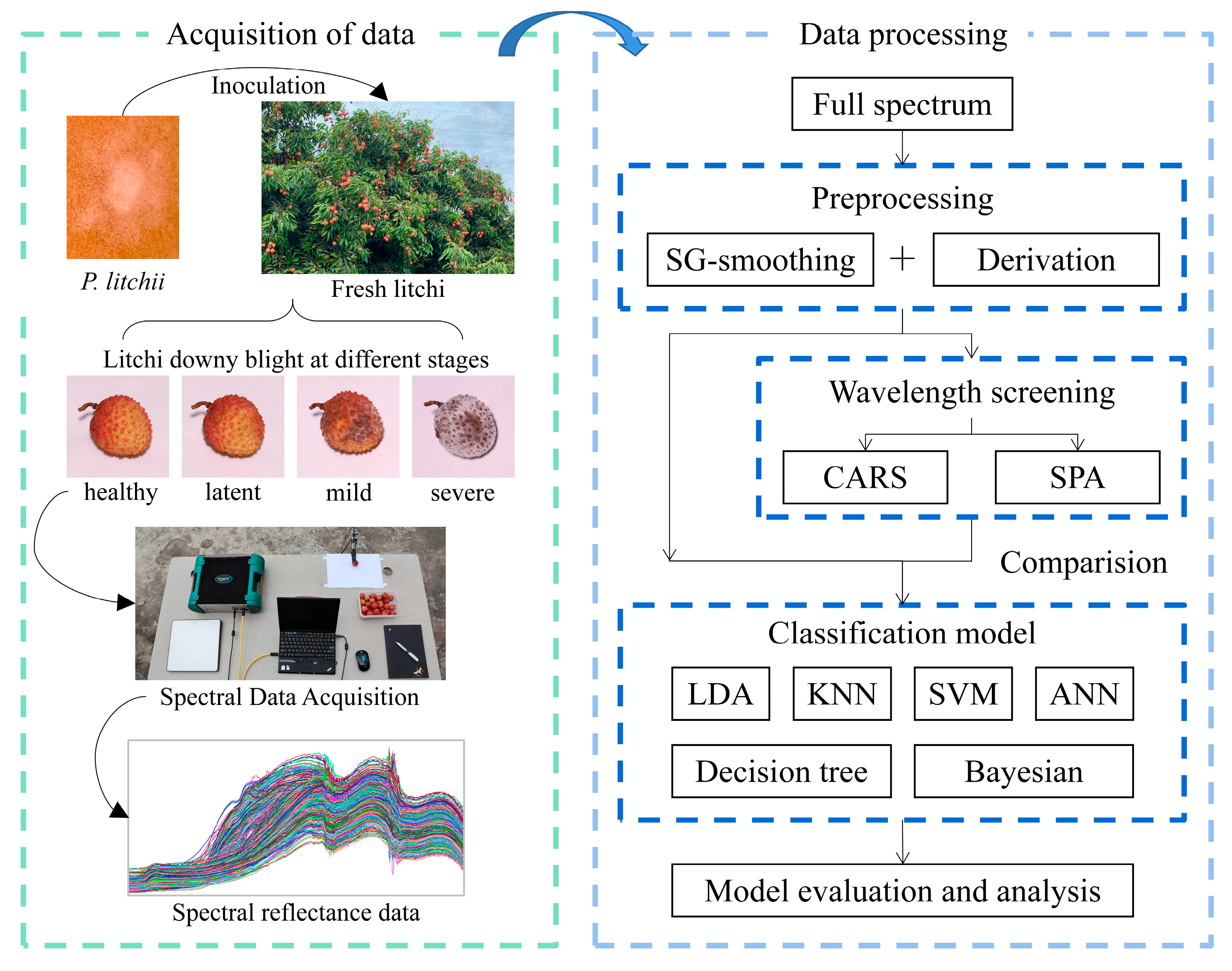
In summary, the purpose of this study is to provide a nondestructive litchi downy blight identification method based on spectral data analysis, which can classify litchi fruits infected with downy blight at different severities, including healthy, latent, mild and severe infections. The methodology of this study is as follows (Figure 1):

(1)

Through scientific and reliable experiments, the diffuse reflectance spectral dataset of litchi fruits with different stages of downy blight infection was collected as the basis for the following research and analysis.

(2)

To simplify the spectral data and make the model more efficient, two different methods of characteristic wavelength screening, CARS and SPA, were evaluated using different preprocessing parameters.

(3)

Six different classification models were evaluated and tested to realize nondestructive identification of litchi downy blight at different stages. Then, the model that performed best was identified through comparisons.

2. Materials and Methods

2.1. Inoculation and Cultivation of Litchi Downy Blight

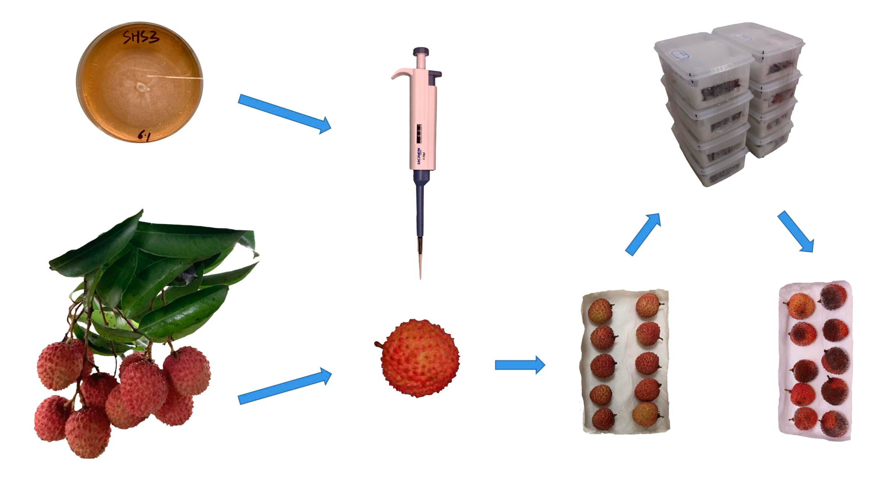
The inoculation and cultivation experiment of litchi downy blight was carried out in the China Litchi and Longan Industry Technology Research System Integrated Laboratory, College of Engineering, South China Agricultural University, in July 2021. The tested strain of P. litchii was SHS3, which was stored in the College of Natural Resources and Environment, South China Agricultural University. The tested litchi fruits were harvested from the litchi orchard at the Institute of Fruit Tree Research, Guangdong Academy of Agricultural Science. Before inoculation, the strain was activated in fresh carrot agar medium, and then, after 5 days of cultivation, a fresh colony of P. litchii was obtained. Sterilized water (5 mL) was added to the colony and shaken gently to obtain a sporangial suspension. Meanwhile, the litchi fruits were incubated in the sterile environment of the lab for over 48 h before the experiment to confirm that they were heathy. Afterwards, healthy litchi fruits of moderate size were selected, ensuring that their surface was clean and dry, and placed in a crisper box. Then, 0.05 mL of sporangium suspension was drip-inoculated using a pipettor onto the epidermal centre of each litchi fruit. The inoculated fruits were placed in an incubator at 25 °C for moisturizing cultivation. The specific processes of the inoculation and cultivation experiment are shown in Figure 2.

All litchi samples were ensured to be healthy before inoculation, and litchi downy blight was inoculated and cultivated using scientific procedures. Thus, all subsequent changes in litchi samples were due to litchi downy blight, including color changes, disease spots, white downy mildew and some other surface properties.

2.2. Spectral Data Acquisition

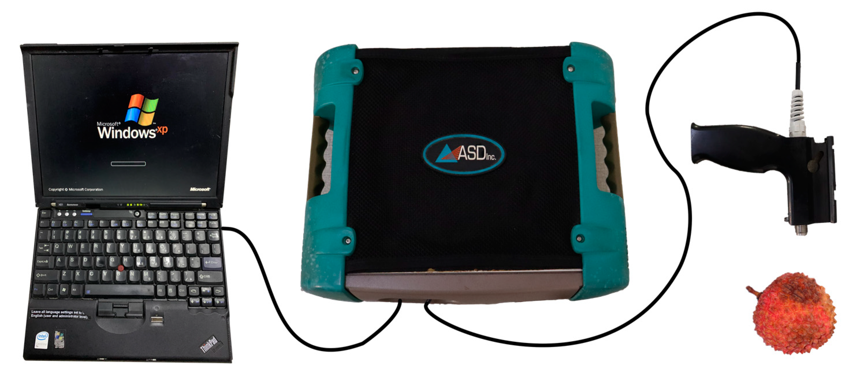
Spectral data acquisition of litchi downy blight was conducted in July 2021 in the outdoor space of South China Agricultural University. Spectral data, ranging from 350–1350 nm, of litchi fruits inoculated with P. litchii were collected by an ASD Field Spec 3 Portable Spectroradiometer (Analytical Spectral Devices, Inc., Boulder, CO, USA). The instrument is sensitive to visible and near-infrared light, has a spectral sampling interval of 1.377 nm and has a spectral resolution of 3 nm at 700 nm [18]. During data acquisition, an optical fibre probe with a 25° field of view was equipped and placed 2 cm vertically above the litchi sample to be measured. In particular, we ensured that there were no other miscellaneous objects in the field of view of the probe and that the amount of sunlight was sufficient. Three spectral data curves were collected for each litchi sample. The process of spectral data acquisition is shown in Figure 3. The first spectral data acquisition was carried out before inoculation; thereafter, spectral data were acquired every 24 h. Moreover, litchi samples were continuously observed, especially the progression of symptoms and growth of white downy mildew, until the litchi samples were severely infected, at which time the last spectral data were acquired. Finally, a total of 7 spectral data acquisitions were accomplished.

2.3. Disease Stages of Downy Blight

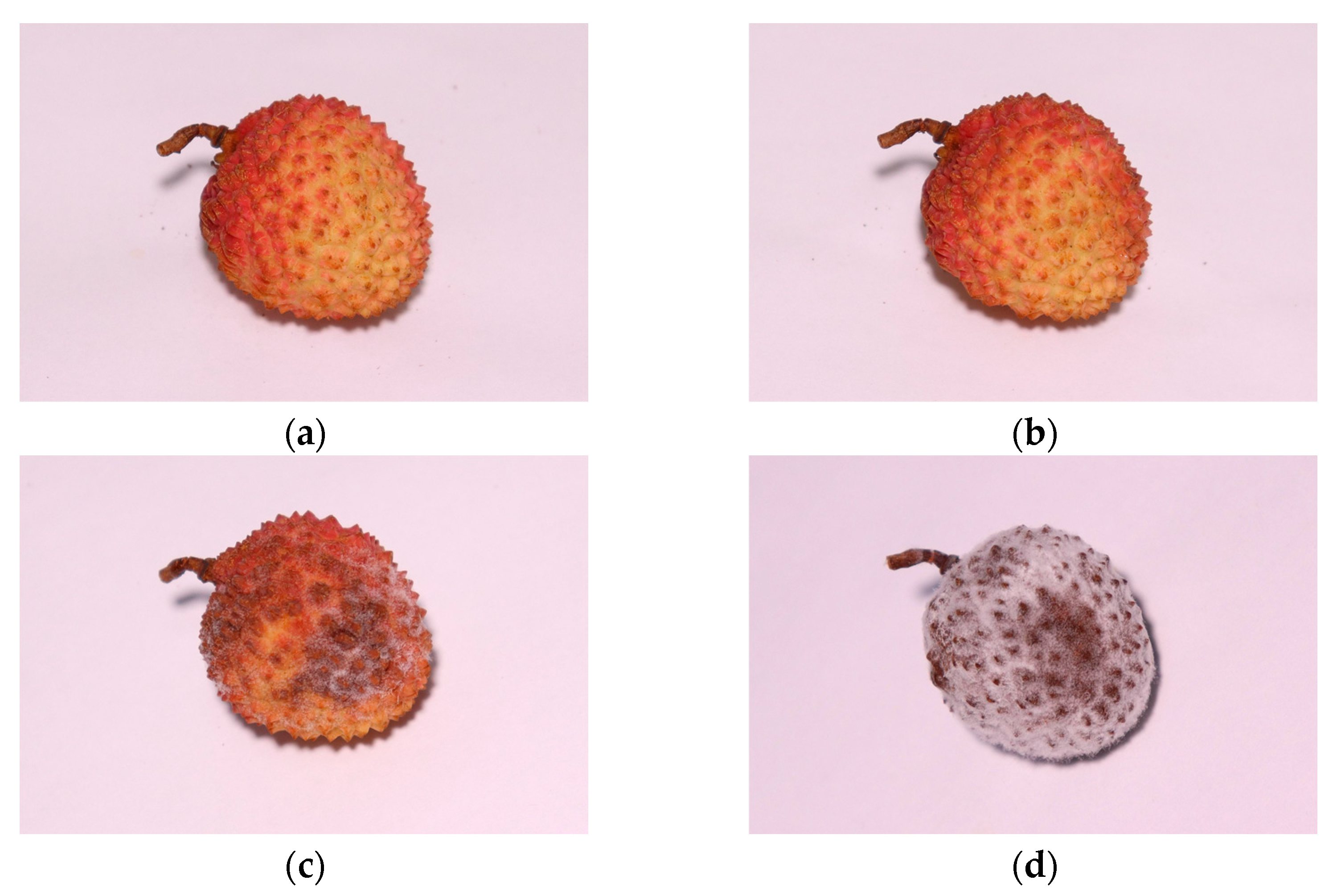
The disease stages of litchi downy blight were divided into 4 categories: healthy, latent, mild and severe. Before the experiment, all litchi samples were observed for 36 h to ensure healthy conditions. The latent category was defined as the period between inoculation with P. litchii and the first appearance of prominent lesion spots. As shown in Figure 4, the mild category refers to visible brown lesion spots on the surface of litchi fruit accounting for 10–30% of the surface area. The severe category refers to the surface of litchi fruit being totally browned and covered with white downy mildew.

Principally, the division of different disease stages was based on the duration of inoculation of P. litchii; however, due to experimental error and individual differences between litchi fruit samples, the actual disease progression of each sample was slightly different. Therefore, to improve the quality of the data, agricultural experts were also invited to evaluate the stages of individual litchi samples through images to calibrate the division results. Samples whose disease stage was difficult to accurately define were discarded. Finally, a total of 609 data points were obtained and are shown in

Table 1. Distribution of the dataset.

Healthy	Latent	Mild	Severe	Total
121	186	109	193	609

.

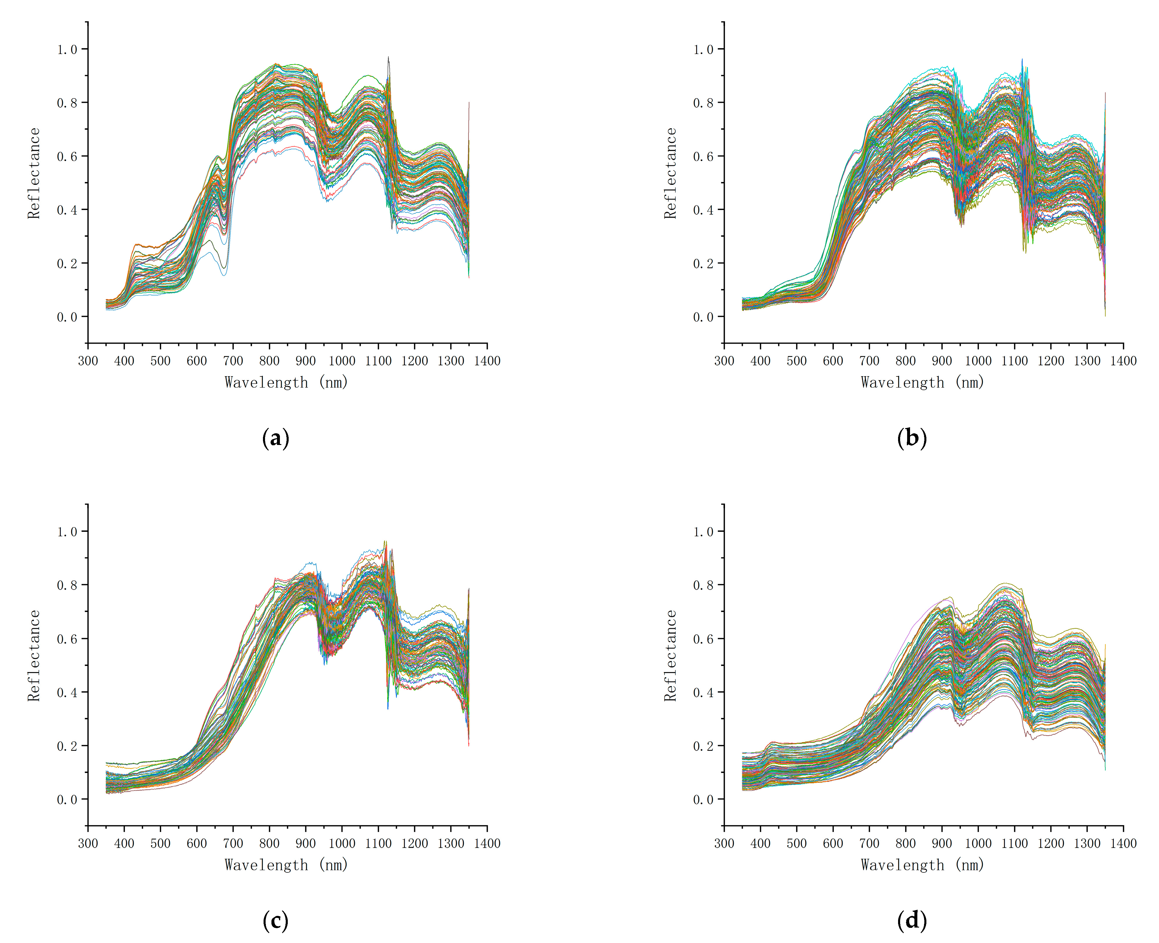
2.4. Spectral Data Preprocessing

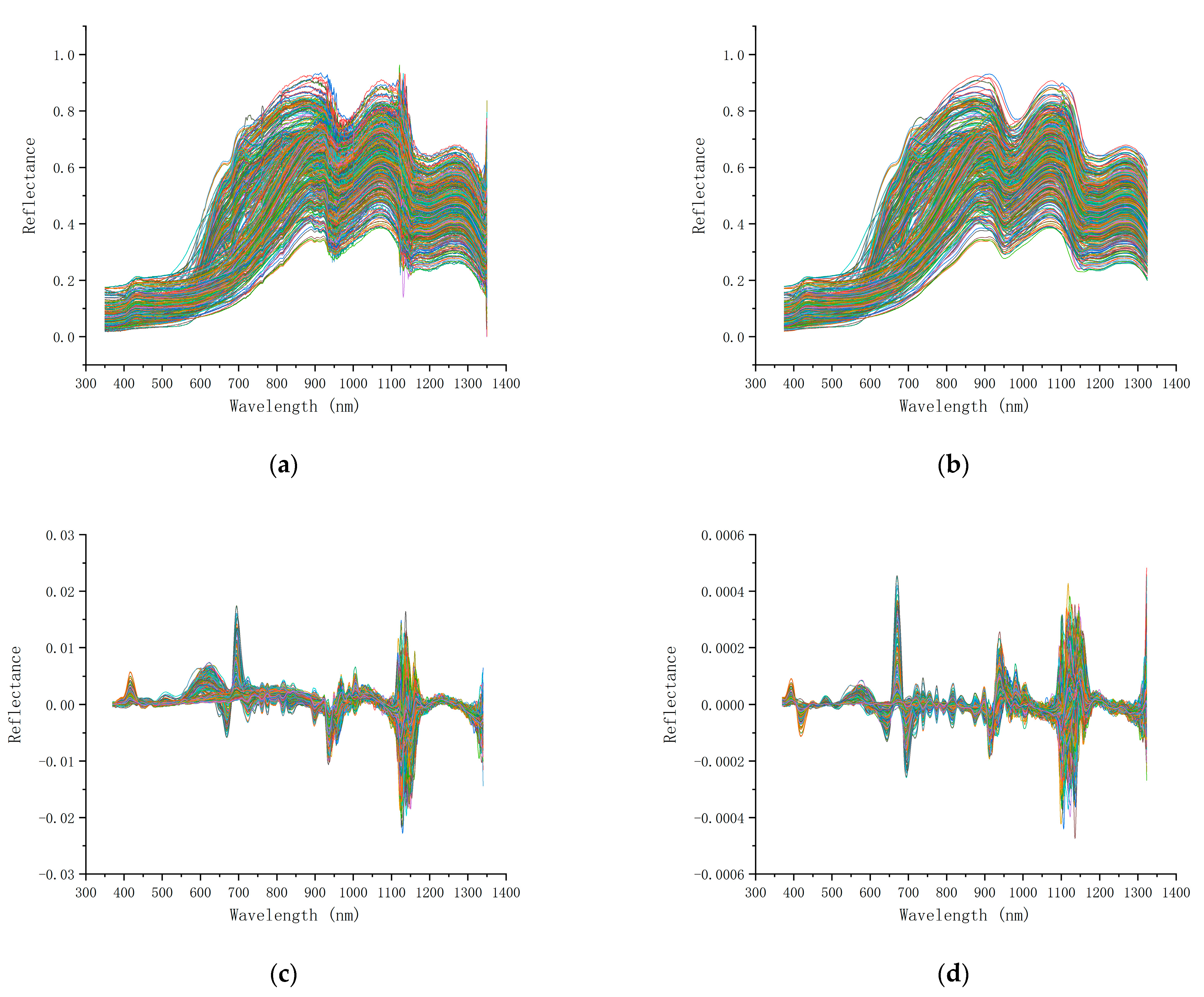
The original spectral data not only contained the characteristic spectrum of the tested litchi sample but also contained noise data such as high-frequency random noise and baseline drift. Moreover, they are also affected by the physical properties of the samples, such as viscosity, particle size, surface texture and density. Therefore, before using spectral data for sample attribute analysis, pretreatment should be carried out first to achieve noise reduction and reduce the interference of other influencing factors.

2.4.1. Savitzky–Golay Smoothing

The Savitzky–Golay (SG) smoothing method is a widely used spectral denoising method. Compared with traditional methods, such as moving average smoothing, this method emphasizes the central role of the centre point. The principle of SG smoothing is to set a smoothing frame in advance, use the weighted average method to carry out polynomial least square fitting to the data in the moving frame, and then use the convolution calculation method to move the frame backwards to complete the smoothing processing of all data [19].

The smoothing effect varies with the size of the smoothing frame. The larger the frame size is, the more significant the smoothing effect but the greater the possibility of losing useful information. In this study, different smoothing frame sizes ranging from 31–51 and different polynomial orders ranging from 2–4 were tested.

2.4.2. Derivation

The derivative method can be used to eliminate the influence of baseline drift or gentle background, which is beneficial to improve the resolution and sensitivity of spectral data. However, if the signal-to-noise ratio (SNR) of the original spectral data is not high enough, the derivation will further amplify the noise signal and adversely affect the analysis. Therefore, the derivative method was combined with the SG smoothing method. The SG smoothing method is a polynomial fitting, and the weighted average expression of the frame centre required by the derivation of the polynomial can be obtained. The derivative coefficient can be obtained by least square calculation. The specific calculation method is as follows

$${\mathrm{x}}_{\mathrm{i}}\prime =\frac{1}{A}{\displaystyle {\sum }_{j=-m}^m{w}_j{x}_{i+j},\begin{array}{cc}& \end{array}i=}1,...,n-2m$$

(1)

where the smoothing frame size is $2 m+1$, $A$ is the normalization constant, $x_i\prime$ is the smoothing data of spectral data $x_i$, $w_j$ is the corresponding derivative coefficient, and $w_j$ is determined after the frame size is determined. The purpose of multiplying each measured value by the derivative coefficient $w_j$ is to minimize the effect of smoothing on the useful information, and $w_j$ is obtained by polynomial fitting based on the least square principle. The smoothing effect varies with the differentiation order. In this study, different differentiation orders ranging from 0–2 were tested. After smoothing, the spectral data will lose $m$ wavelengths at both ends, and the remaining wavelengths correspond to each original data point. Therefore, smoothing will not affect the feasibility of the following further analysis in practical applications.

2.5. Characteristic Wavelength Screening

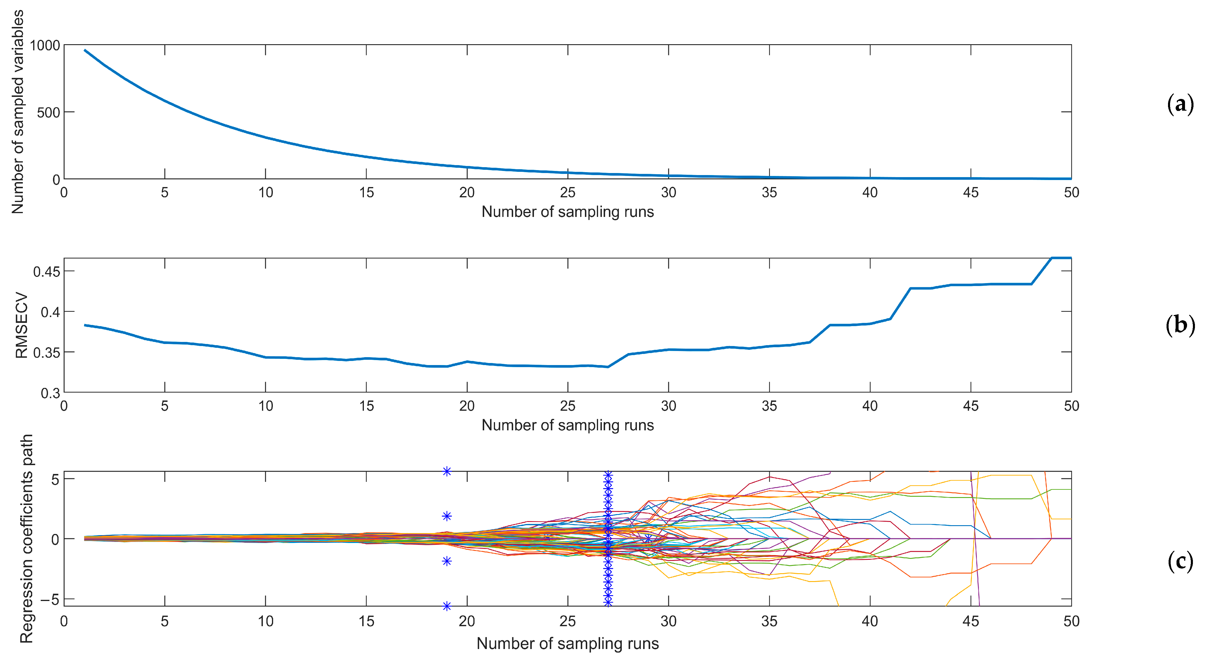
2.5.1. Competitive Adaptive Reweighted Sampling

CARS is a characteristic wavelength screening method combining Monte Carlo sampling and the regression coefficient of the PLS model, imitating the principle of “survival of the fittest” in Darwinian evolution theory [20]. In the CARS algorithm, points with a large absolute weight of the regression coefficient in the PLS model were reserved as new subsets through adaptive weighted sampling (ARS) each time, and points with small weights were removed. Then, the PLS model was established based on the new subsets. After several calculations, the wavelengths in the subset of the minimum root mean square error (RMSECV) of the PLS model were selected as the characteristic wavelengths.

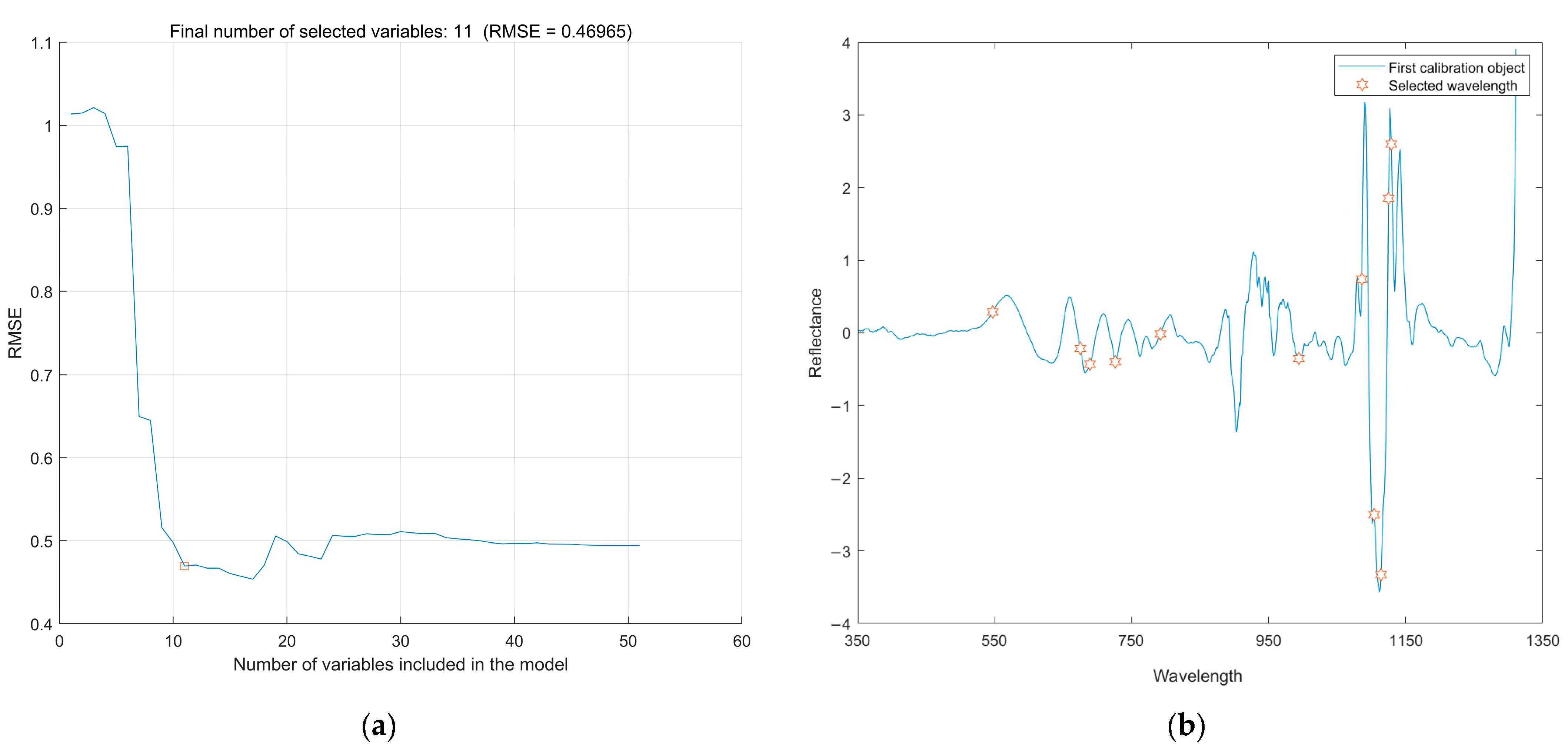
2.5.2. Successive Projections Algorithm

SPA is a forward selection variable method of characteristic wavelength screening. By using projection analysis of vectors, the wavelength is projected onto other wavelengths, and the size of the projections is compared [21]. The wavelength with the largest projection vector is selected as the wavelength to be selected, and then the final characteristic wavelengths are selected based on the correction model. SPA selects the combination of variables with the least redundant information and the least collinearity. The main steps of the algorithm are as follows.

The initial iteration vector is denoted as $x_{k\left(0\right)}$, the number of variables to be extracted is $N$ and the number of columns of the spectral matrix is $J$. Any one column in the optional spectral matrix is denoted as column $j$, and we assign column $j$ of the modelling set to $x_j$, denoted as $x_{k\left(0\right)}$.

The set of unselected column vector positions was denoted as $s$

$$s=\left\{j,1\le j\le J,j\notin \left\{k\left(0\right),...,k\left(n-1\right)\right\}\right\}$$

(2)

The projection of $x_j$ to the remaining column vectors was calculated separately $P_{x_j}$

$$P_{x_j}=x_j-\left(x_j^T{x}_{k\left(n-1\right)}\right)x_{k\left(n-1\right)}{\left(x_{k\left(n-1\right)}^T{x}_{k\left(n-1\right)}\right)}^{-1},j\in s$$

(3)

The spectral wavelength of the largest projected vector was extracted

$$k\left(n\right)=\arg \left(\max \left(\Vert P_{x_j}\Vert \right),j\in s\right)$$

(4)

To make $x_j=P_{x_j}, j\in s$, when $n\le N$, the rule $n=n+1$ was applied, and then loop calculations were performed.

Finally, the extracted variables were $\left\{x_{k\left(n\right)}=0,...,N-1\right\}$, corresponding to $k\left(0\right)$ and $N$ in each cycle. Multivariable linear regression (MLR) models were built separately, and the root mean squared error (RMSE) for the interactive validation of the model was obtained. For different candidate characteristic subsets, the values of $k\left(0\right)$ and $N$ corresponding to the smallest RMSE value were the optimal values.

2.6. Classification Models

To correctly evaluate the spectral data corresponding to different disease stages of litchi downy blight, the problem was approached as a classification problem. When a group of litchi spectral data is obtained, the model can automatically determine which data point is healthy, latent, mild or severe to complete the identification of the disease stages of litchi downy blight. There are many classification models that can achieve such tasks, such as decision trees, LDA, naive Bayesian classifiers, KNN, SVMs and ANNs.

The decision tree algorithm [22] uses a tree structure and layer reasoning to achieve the final classification. The amount of calculation is relatively small, and it is easy to convert into classification rules. In this study, the split criterion was set as gin’s diversity index, and the maximum number of splits was 20.

LDA [23] finds the optimal projection direction, projects the points in the high-dimensional space to the low-dimensional space, and then reclassifies the low-dimensional space. Generally, for linearly separable samples, LDA makes the samples remain linearly separable after dimensionality reduction through a projection direction, the distance between samples of different categories is as far as possible, and the same sample is as concentrated as possible.

The idea of the naive Bayesian classifier [24] is to treat the spectral characteristic vector of the classified sample, calculate the probability of each category under the condition of the spectral characteristic vector, and consider the sample to be classified as the category with the highest probability. In this study, the numeric predictors are set as the kernel, and the kernel type is set as Gaussian.

KNN [25] is a nonparametric method, the idea of which is that if most of the samples have similar K values in the feature space (that is, the closest neighbors in the feature space) belong to a certain category, the sample also belongs to this category. In this study, the distance metric was set as a cosine, and the number of neighbors was 10.

The basic idea of SVMs [26] is to construct an optimal decision hyperplane in the feature space, which maximizes the distance between the hyperplane and the nearest samples of different classes. SVMs are suitable for solving the problem of high-dimensional classification of small samples. In this study, the kernel function of the SVM was set as quadratic.

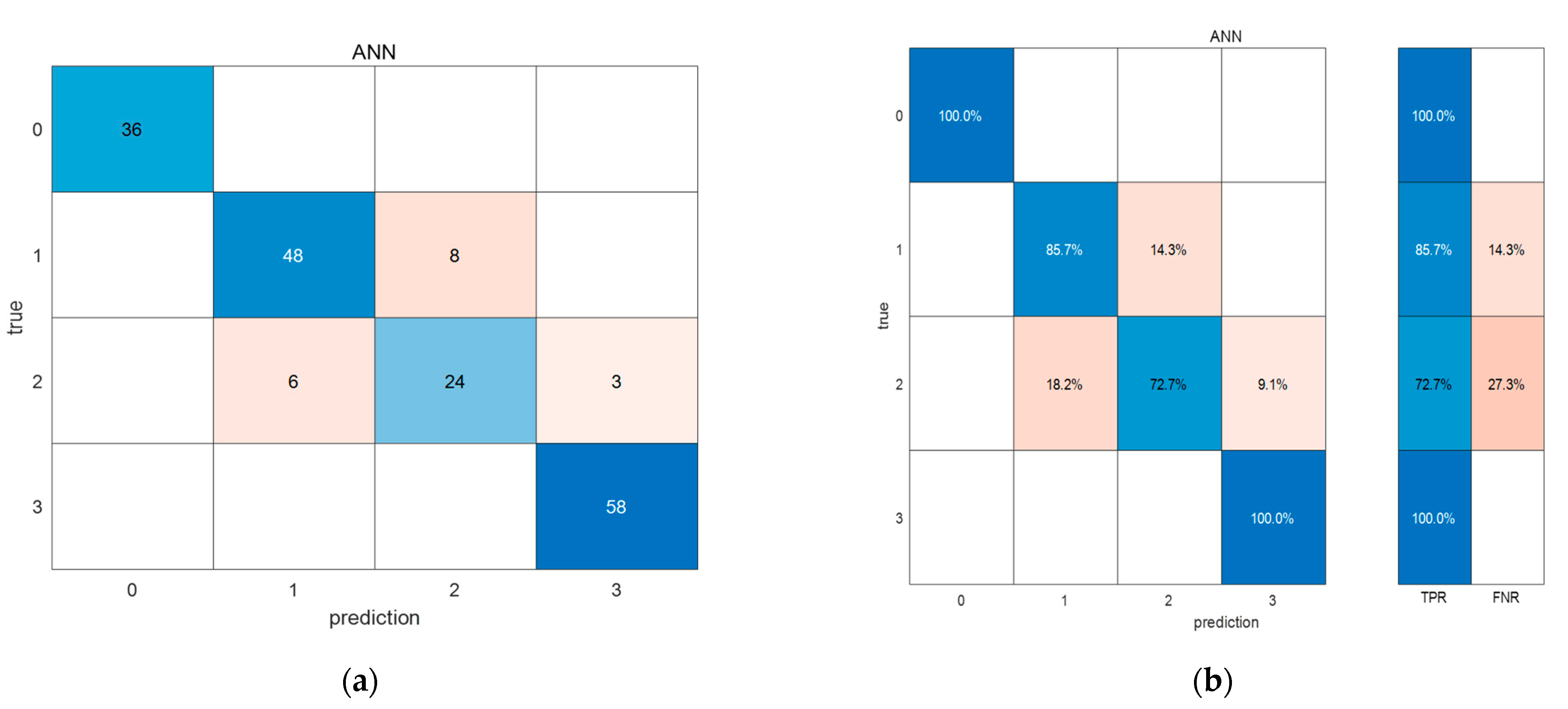
ANNs are designed based on the research results of biological neural networks and are systems composed of many simple processing units working in parallel. The ANN function depends on the structure of the network, the connection strength and the processing mode of each unit. ANNs have great potential in information processing. In this study, the type of ANN was a wide neural network, and the number of fully connected layers was one, with a layer size of 100. The activation function was ReLU, the iteration limit was 1000, and the regularization strength (lambda) was 0.

In summary, the classification models were used to identify the spectral data of litchi downy blight at different disease stages. In this study, both the original full-band spectral data and the selected characteristic wavelength data were tested, and their accuracy calculated and compared.

All of the analytical procedures used in this study were performed with algorithms developed in MATLAB vR2021a software; specifically, the classification models were analysed using the Statistics and Machine Learning Toolbox (Version 12.1).

3. Results

3.1. Spectral Data Characteristics of Litchi Downy Blight

The pathogenic process of litchi downy blight developed rapidly after inoculation with P. litchii, and it only took 5 days to achieve the severe stage. The figures show the original spectral data corresponding to samples at different disease stages of litchi downy blight. Overall, the trend of the spectral curves was basically consistent, indicating that the experiment is reliable. The characteristics of spectral curves corresponding to different disease stages were significantly different, especially in the range of 400–950 nm, which covers visible and near-infrared light (Figure 5). Therefore, it is feasible to distinguish different disease stages of litchi downy blight through spectral data.

Litchi fruits of the healthy category of downy blight had abundant spectral reflection in the visible light range, showing a reflection peak at approximately 660 nm, reflecting the red color characteristic of litchi fruits and forming a platform characteristic at 750–930 nm (Figure 5a).

During the latent category of downy blight, the litchi fruit surface began to show slight browning, which was difficult to detect by visual observation. The spectral curve of litchi fruit in the range of 600–930 nm was smoother than that of healthy fruit, showing an upwards convex curve in general, especially the small wave valley at 685 nm, which decreased or even disappeared (Figure 5b).

When the mild category of downy blight was present, there were obvious dark brown spots on the surface of litchi fruits, with white downy mildew present around the spot area. The reflectance of the spectral curve in the range of 600–930 nm was lower than that of the latent category, and the slope was close to 1 (Figure 5c).

The surface of litchi fruit of the severe category of downy blight was completely brown and covered with a thick layer of white downy mildew. The reflectance of the spectral curve decreased further in the range of 700–930 nm but increased in the range of visible light, which was inferred to be related to the significant change in the surface color characteristics of litchi fruit (Figure 5d).

In addition, in the near-infrared spectrum range of 950–1350 nm, the spectral data corresponding to different disease stages of downy blight showed little difference. At approximately 1150 nm, relatively obvious noise was observed. This noise existed in the spectral data of all samples and was relatively uniform. Therefore, noise was not considered to affect the subsequent experimental analysis.

3.2. Result of Spectral Data Preprocessing

The original spectral data without processing have a large number of fluctuations caused by high-frequency noise, showing a jagged shape on the spectral curve. In addition, due to the difference in ambient light in different samples and the scattering influence brought by sample surface granularity, although the equipment was calibrated in time during the experiment, there was still a certain difference in the amplitude of the spectral curve (Figure 6a).

The original spectral data were processed by SG smoothing, the sawtooth on the spectral curve was reduced, the curve became smoother, and the noise was reduced. Moreover, the original trend and characteristics of the spectral curves were preserved. In particular, the noise near 1150 nm was substantially reduced, which sufficiently reflected the effect of smoothing (Figure 6b).

Additionally, the original spectral data were processed by first and second derivatives with the SG smoothing method, which greatly reduced the difference in the amplitude of the spectral curve and made all curves more concentrated. The smoothing process of spectral data also plays a role in normalization, and the absolute value difference between different spectral curves can be weakened, while the relative value difference can be prominent. Among them, the normalization effect of data smoothed by the second derivative was better than that achieved by the first derivative, and all curves were clustered near each other, which simplified and stabilized subsequent operations. The positions with large curve fluctuations reflect the differences of different curves, and these positions are also more likely to have characteristic wavelengths (Figure 6c,d).

In conclusion, smoothing processing can effectively reduce the impact of noise on spectral data and helps the subsequent selection of characteristic wavelengths and the establishment of an analysis model [27]. However, in the process of smoothing, the selection of key parameters is also very important, and parameter selection will be further discussed in the following paragraphs.

3.3. Characteristic Wavelength Sensing Results

3.3.1. Result of Key Parameter Selection

In the experimental process, it was found that when derivations with the SG smoothing method were used to preprocess spectral data, different key parameters not only had a direct impact on the shape of the spectral curve but also had a significant impact on the subsequent results of characteristic wavelength screening. Among them, different frame sizes, polynomial orders and differentiation orders had a decisive influence on data smoothing and subsequent characteristic wavelength screening. Thus, orthogonal experiments were designed for these parameters to optimize the combinations. Through a certain pretest, three levels of smoothing frame size were selected, 31, 41 and 51; three levels of polynomial order were selected, 2, 3 and 4; three levels of differentiation order were selected, 0, 1 and 2. In summary, an orthogonal experiment with three factors and three levels was designed, with a total of nine groups of experiments. Then, on the basis of the results of each group of experiments, CARS and SPA were used to select characteristic wavelengths, and the corresponding number of characteristic wavelengths was obtained, as shown in

Table 2. Orthogonal experiments of parameter combinations in preprocessing and the corresponding number of characteristic wavelengths obtained using CARS and SPA.

	Frame Size	Polynomial Order	Differentiation Order	CARS	SPA
①	31	2	0	146	37
②	31	3	2	41	21
③	31	4	1	60	22
④	41	2	2	36	11
⑤	41	3	1	99	26
⑥	41	4	0	113	44
⑦	51	2	1	68	32
⑧	51	3	0	77	25
⑨	51	4	2	87	26

.

It can be seen from the experimental results that the influence of different parameter combinations on the selection of characteristic wavelengths was significant. Overall, the results of CARS and SPA showed the same variation trend under different parameter combinations, but the result of SPA was better than that of CARS in each group. Among them, the best results all appeared in group ④, where the smoothing frame size was 41, the polynomial order was 2, and the differentiation order was 2. CARS selected 36 wavelengths, and SPA selected 11 wavelengths.

3.3.2. Result of Competitive Adaptive Reweighted Sampling

The process of CARS characteristic wavelength screening was as follows. After repeated comparison, Monte Carlo sampling times were set to 50 in this study [28]. As shown in Figure 7a, with increasing sampling times, the number of selected wavelengths gradually decreased. As shown in Figure 7b, RMSECV gradually decreased and then gradually increased after reaching the lowest point. It is generally believed that the decline in RMSECV reflects the removal of invalid information in spectral data, while the rise in RMSECV reflects the removal of effective information in spectral data. Therefore, the lowest RMSECV was selected as the result. The positions marked by solid vertical lines in Figure 7c represent the regression coefficients of each variable when RMSECV reached the minimum value. At this time, the sampling ran 27 times, and the number of characteristic wavelengths selected by CARS was 36.

3.3.3. Result of Successive Projections Algorithm

The process of applying SPA to characteristic wavelength screening was as follows. SPA determined the number of characteristic wavelengths based on RMSE. As shown in Figure 8a, when the number of wavelengths increased from 1 to 11, the RMSE decreased rapidly and then plateaued after a slight fluctuation. Through experiments, it was found that RMSE tended to flatten after a rapid decline, and the RMSE changed very little at this time. If the minimum RMSE point was pursued, the number of characteristic wavelengths increased to varying degrees. Therefore, a point that was not significantly greater than the minimum RMSE was selected as the result according to the F test in this study to optimize the characteristic wavelength screening process [29]. Finally, 11 wavelengths were selected as characteristic wavelengths, and the specific distribution is shown in Figure 8b. The characteristic wavelengths were mainly distributed in the visible spectral range of 550–760 nm and the near-infrared spectral range of 1100–1150 nm.

3.3.4. Result of Characteristic Wavelengths

By observing the characteristic wavelength distribution corresponding to the characteristic wavelength selection test results, it was found that the characteristic wavelengths selected by CARS were relatively scattered, with many consecutive adjacent wavelengths and more redundancy, which had a relatively poor performance.

The characteristic wavelengths selected by SPA were mainly distributed in the visible spectral range of 560–760 nm and the near-infrared spectral range of 1100–1150 nm, which corresponded to the regions with large fluctuations, as shown in Figure 6d, with fewer numbers and better effects. Therefore, 11 wavelengths selected by SPA in group ④ of the experiment shown in Table 2 were finally confirmed as characteristic wavelengths for subsequent analysis [30]. The selected characteristic wavelengths are shown in

Table 3. Characteristic wavelengths.

Method	Selected Wavelength (nm)
CARS	426, 549, 550, 637, 638, 639, 689, 707, 708, 727, 728, 739, 740, 746, 806, 811, 812, 817, 831, 832, 833, 834, 902, 903, 984, 997, 1011, 1026, 1075, 1192, 1208, 1224, 1275, 1284, 1292, 1295
SPA	567, 695, 709, 746, 812, 1014, 1106, 1124, 1134, 1145, 1149

.

3.4. Result of Classification Models

In this study, full-band spectral data and 11 characteristic wavelengths selected by SPA were tested to compare the effects of different classification models. As shown in

Table 4. Partitioning of the training set and test set.

	Quantity	Percentage
train	426	70%
test	183	30%
total	609	100%

, 70% of all 609 data points were used as training data, and 30% were used as test data. Considering the small training set, cross-validation was adopted in the training process, and the number of cross-folds was 15.

The data of the training set were imported into a decision tree, LDA, a naive Bayesian classifier, KNN, an SVM and an ANN. After the training, the model was tested with the test set, and the accuracy of different classification models was calculated. Accuracy P was calculated as follows, where T represents the total number of samples in the test set and C represents the number of correctly classified samples in the test set.

$$P=\frac{C}{T}\times 100\%$$

(5)

Finally, the accuracy of each classification model is shown in

Table 5. The accuracy of each classification model.

Model	Full Wavelengths		11 Selected Wavelengths
	Validation	Test	Validation	Test
Decision Tree	91.5%	87.4%	92.0%	82.5%
LDA	89.9%	94.5%	88.5%	80.3%
Naive Bayes	90.1%	83.6%	93.0%	86.3%
KNN	91.5%	93.4%	91.8%	84.2%
SVM	99.5%	96.2%	94.8%	89.6%
ANN	99.5%	97.3%	91.8%	90.7%

. In general, the accuracy of the test set reached a good level, which had reference significance for practical production practice. Among them, the average accuracy of the test set of full-band spectral data was 92.1%, and the average accuracy of the test set of 11 characteristic wavelengths selected by SPA was 85.6%. By selecting characteristic wavelengths, 1001 wavelengths were replaced by 11 wavelengths, and the number of wavelengths was only 1.1% of the original. Even if the number of wavelengths was greatly reduced, the accuracy of the classification model was only reduced by 6.5 percentage points, and the performance of classification was basically not reduced, which fully embodied the value of preprocessing with SG smoothing and the SPA algorithm.

Specifically, the best classification models were the SVM and ANN. The accuracy of the test set of the full-band spectral data reached 96.2% and 97.3%, and the accuracy of the test set of the 11 characteristic wavelengths reached 89.6% and 90.7% for the SVM and ANN, respectively.

For further analysis of the ANN model, with the highest accuracy of 90.7% in the test set, 11 characteristic wavelengths were used. Through a confounding matrix, the accuracy of categories of health, latent, mild and severe were 100%, 85.7%, 72.7% and 100%, respectively (Figure 9).

In the classification and recognition of litchi downy blight, the classification model can recognize and classify health and severe categories well, but it may misidentify the latent and mild categories to some extent. This result is because both the healthy and severe categories have distinct and definite characteristics that are relatively easy to accurately evaluate. However, the latent and mild categories were the transition state in the process of change, and the characteristics were relatively obscure, so they were more difficult to classify.

4. Discussion

According to the results shown above, the nondestructive testing method based on the spectral analysis proposed in this paper has unique advantages in the detection of litchi downy blight. On the one hand, compared with the image recognition method based on visible light images, the spectral method has higher sensitivity and accuracy, enabling the identification of the early stage of litchi downy blight and classification of different disease stages. Imaging methods are unable to easily perform this identification and classification. On the other hand, compared with traditional biochemical or molecular detection methods, the spectral method is more intelligent and shows potential to achieve the nondestructive identification of litchi downy blight at different stages.

In the analysis of spectral data in this paper, the SG smoothing method was used for pretreatment and was found to be effective. Additionally, the noise caused by the environment, equipment and other factors in the original spectral data can be effectively reduced. Smoothing and denoising were essential in the processing of spectral data analysis. Notably, several parameters, such as frame size, polynomial order and differentiation order, affected the smoothing results. In general, excessive smoothing resulted in the loss of some information. Therefore, there was a balance to be achieved.

The original spectral data of litchi downy blight collected in this paper cover a wide range of wavelengths from 350–1350 nm; however, the large amount of spectral data is unacceptable in practical applications due to the associated cost. Thus, the selection of characteristic wavelengths is very constructive. CARS and SPA are typical characteristic wavelength screening methods. In this paper, SPA performed better, as also reported in other studies [31]. Moreover, our results confirmed that characteristic wavelength screening can improve the efficiency of the applied model because the quantity of spectral data significantly reduced.

Of the 11 characteristic wavelengths selected, four belonged to the visible band, which was distributed in the region of red and yellow light. Visible light is often used for color evaluation and pigment analysis. With the infection of downy blight, the surface of litchi gradually changed from red to brown and white, indicating that the spectroscopy analysis could be used to identify downy blight by obtaining the color and pigment information [32]. The other seven characteristic wavelengths belonged to near-infrared bands, and the correlation between these wavelengths and litchi downy blight was difficult to determine, but it was inferred to be related to the following factors. When infected with downy blight, the epidermis of litchi became softer, stickier, smoother and moister. Furthermore, the inside of litchi fruit began to rot when severely infected. Theoretically, the NIR spectrum is sensitive to these changes, which can be beneficial for identifying litchi downy blight.

In this paper, the last and most important step of spectral data analysis was to classify spectral data with classification models. Studies in many other fields have verified that classification models have strong analytical ability. In our identification of litchi downy blight based on spectral data, it was also verified that classification models perform well. The excellent performance of ANNs, as advanced deep learning tools, was expected.

5. Conclusions

This study was the first to complete the exploration of applying the diffuse reflectance spectrum data analysis method to the intelligent identification of litchi downy blight and confirmed that the classification and judgement of different disease stages of litchi downy blight can be realized by analyzing diffuse reflectance spectrum data with certain methods. By preparing experimental materials and collecting experimental data, a controlled and scientific dataset of litchi downy blight was obtained, including the spectral data of different categories of healthy and latent, mild and severe infection. In data analysis, SG smoothing and the derivation method were combined to preprocess the original data, and then CARS and SPA characteristic wavelength screening methods were compared. The experiment showed that the SPA method had better performance after optimizing the parameters. Afterwards, 11 characteristic wavelengths were selected, accounting for only 1.1% of the original data. Finally, the characteristic wavelengths were imported into different classification models for training, and their accuracy was tested. Decision tree, LDA, naive Bayesian classifier, KNN, SVM and ANN methods were compared, and the ANN model was the best, with an accuracy of 90.7%. The above work laid a theoretical foundation for diffuse reflectance spectroscopy in the identification of litchi downy blight and provided a reference for its application in practical production. An improvement in the precise control of litchi downy blight is beneficial to promote a reduction in chemical use and improvements in the yield and quality of litchi. Litchi producers obtain greater economic benefits, litchi consumers obtain more delicious high-quality litchi, and the litchi industry continues to develop well.

References

1. Qi, W.; Chen, H.; Luo, T.; Song, F. Development Status, Trend and suggestion of litchi industry in mainland China. Guangdong Agric. Sci. 2019, 46, 132–139. [Google Scholar] [CrossRef]
2. Zhang, J.; Zhu, F.; Gu, M.; Ye, H.; Gu, L.; Zhan, L.; Liu, C.; Yan, C.; Feng, G. Inhibitory activity and action mechanism of coumoxystrobin against Phytophthora litchii, which causes litchi fruit downy blight. Postharvest Biol. Technol. 2021, 181, 111675. [Google Scholar] [CrossRef]
3. Ye, W.; Wang, Y.; Shen, D.; Li, D.; Pu, T.; Jiang, Z.; Zhang, Z.; Zheng, X.; Tyler, B.M.; Wang, Y. Sequencing of the Litchi Downy Blight Pathogen Reveals It Is a Phytophthora Species with Downy Mildew-Like Characteristics. Mol. Plant Microbe Interact. 2016, 29, 573–583. [Google Scholar] [CrossRef] [Green Version]
4. Kong, G.; Feng, D.; Li, W.; Lian, S.; Xi, P.; Jiang, Z. Research progress in studies on the downy blight disease in litchi. J. Fruit Sci. 2021, 38, 603–612. [Google Scholar] [CrossRef]
5. Zhang, D.; Fang, H.; He, Y. Research of crop disease based on visible/near infrared specttral image technology: A Review. Spectrosc. Spect. Anal. 2019, 39, 1748–1756. [Google Scholar] [CrossRef]
6. Bai, B.; Yu, J.; Fu, Z.; Zhang, L.; Li, X. Application of spectral imaging technology for detecting crop disease information: A review. Spectrosc. Spect. Anal. 2020, 40, 350–355. [Google Scholar] [CrossRef]
7. Kai, L.; Zhang, X.; Zhang, X. Early Detection of Cucumber Downy Mildew in Greenhouse by Hyperspectral Disease Differential Feature Extraction. Trans. Chin. Soc. Agric. Mach. 2020, 50, 212–220. [Google Scholar] [CrossRef]
8. Appeltans, S.; Pieters, J.G.; Mouazen, A.M. Detection of leek white tip disease under field conditions using hyperspectral proximal sensing and supervised machine learning. Comput. Electron. Agric. 2021, 190, 106453. [Google Scholar] [CrossRef]
9. Appeltans, S.; Pieters, J.G.; Mouazen, A.M. Detection of Leek Rust Disease under Field Conditions Using Hyperspectral Proximal Sensing and Machine Learning. Remote Sens. 2021, 13, 1341. [Google Scholar] [CrossRef]
10. Liu, S.; Tan, X.; Liu, C.; Zhu, C.; Li, W.; Cui, S.; Du, Y.; Huang, D.; Xie, F. Recognition of fusarium head blight wheat grain based on hyperspectral data processing algorithm. Spectrosc. Spect. Anal. 2019, 39, 3540–3546. [Google Scholar] [CrossRef]
11. Lucas Domingos da Silva, A.; Alves Filho, E.G.; Silva, L.M.A.; Carlos Huertas Tavares, O.; Gervasio Pereira, M.; de Campos, T.; Manoel da Silva, L. Near infrared spectroscopy to rapid assess the rubber tree clone and the influence of maturation and disease at the leaves. Microchem. J. 2021, 168, 106478. [Google Scholar] [CrossRef]
12. Ali, M.M.; Bachik, N.A.; Muhadi, N.A.; Tuan Yusof, T.N.; Gomes, C. Nondestructive techniques of detecting plant diseases: A review. Physiol. Mol. Plant Pathol. 2019, 108, 101426. [Google Scholar] [CrossRef]
13. Zhao, X.; Zhang, J.; Huang, Y.; Tian, Y.; Yuan, L. Detection and discrimination of disease and insect stress of tea plants using hyperspectral imaging combined with wavelet analysis. Comput. Electron. Agric. 2022, 193, 106717. [Google Scholar] [CrossRef]
14. Indrakumari, R.; Poongodi, T.; Khaitan, S.; Sagar, S.; Balamurugan, B. A review on plant diseases recognition through deep learning. In Handbook of Deep Learning in Biomedical Engineering; Academic Press: Cambridge, MA, USA, 2021; pp. 219–244. [Google Scholar] [CrossRef]
15. Mahlein, A.K.; Rumpf, T.; Welke, P.; Dehne, H.W.; Plümer, L.; Steiner, U.; Oerke, E.C. Development of spectral indices for detecting and identifying plant diseases. Remote Sens. Environ. 2013, 128, 21–30. [Google Scholar] [CrossRef]
16. Song, X.; Huang, Y.; Yan, H.; Xiong, Y.; Min, S. A novel algorithm for spectral interval combination optimization. Anal. Chim. Acta 2016, 948, 19–29. [Google Scholar] [CrossRef]
17. Shang, X.; Chisholm, L.A. Classification of australian native forest species using hyperspectral remote sensing and machine-learning classification algorithms. IEEE J. Select. Top. Appl. Earth Obs. Remote Sens. 2014, 7, 2481–2489. [Google Scholar] [CrossRef]
18. Wang, P.; Zhang, J.; Lan, Y.; Zhou, Z.; Luo, X. Radiometric calibration of low altitude multispectral remote sensing images. Trans. CSAE 2014, 30, 199–206. [Google Scholar] [CrossRef]
19. Chen, H.; Pan, T.; Chen, J.; Lu, Q. Waveband selection for NIR spectroscopy analysis of soil organic matter based on SG smoothing and MWPLS methods. Chemom. Intell. Lab. 2011, 107, 139–146. [Google Scholar] [CrossRef]
20. Li, H.; Liang, Y.; Xu, Q.; Cao, D. Key wavelengths screening using competitive adaptive reweighted sampling method for multivariate calibration. Anal. Chim. Acta 2009, 648, 77–84. [Google Scholar] [CrossRef]
21. Araújo, M.C.U.; Saldanha, T.; Galvo, R.K.H.; Yoneyama, T.; Visani, V. The successive projections algorithm for variable selection in spectroscopic multicomponent analysis. Chemom. Intell. Lab. 2001, 57, 65–73. [Google Scholar] [CrossRef]
22. Safavian, S.R.; Landgrebe, D. A survey of decision tree classifier methodology. IEEE Trans. Syst. Man Cybern. 1991, 21, 660–674. [Google Scholar] [CrossRef] [Green Version]
23. Altman, E.I.; Marco, G.; Varetto, F. Corporate distress diagnosis: Comparisons using linear discriminant analysis and neural networks (the Italian experience). J. Bank. Financ. 1994, 18, 505–529. [Google Scholar] [CrossRef]
24. Yager, R.R. An extension of the naive bayesian classifier. Inform. Sci. 2006, 176, 577–588. [Google Scholar] [CrossRef]
25. Keller, J.M.; Grey, M.R.; Givens, J.A. A fuzzy k-nearest neighbour algorithm. IEEE Trans. Syst. Man Cybern. 1985, SMC-15, 580–585. [Google Scholar] [CrossRef]
26. Hearst, M.A.; Dumais, S.T.; Osman, E.; Platt, J.; Scholkopf, B. Support vector machines. IEEE Intell. Syst. 1998, 13, 18–28. [Google Scholar] [CrossRef] [Green Version]
27. Li, L.; Jang, X.; Li, B.; Liu, Y. Wavelength selection method for near-infrared spectroscopy based on standard-sample calibration transfer of mango and apple. Comput. Electron. Agric. 2021, 190, 106448. [Google Scholar] [CrossRef]
28. Guo, P.; Li, M.; Luo, W.; Cha, Z. Estimation of foliar nitrogen of rubber trees using hyperspectral reflectance with feature bands. Infrared Phys. Technol. 2019, 102, 103021. [Google Scholar] [CrossRef]
29. Wang, Z.; Fan, S.; Wu, J.; Zhang, C.; Xu, F.; Yang, X.; Li, J. Application of longwave near infrared hyperspectral imaging for determination of moisture content of single maize seed. Spectrochim. Acta 2021, 254, 119666. [Google Scholar] [CrossRef]
30. Lee, A.; Shim, J.; Kim, B.; Lee, H.; Lim, J. Nondestructive prediction of soluble solid contents in Fuji apples using visible near-infrared spectroscopy and various statistical methods. J. Food Eng. 2022, 321, 110945. [Google Scholar] [CrossRef]
31. Xu, L.; Chen, M.; Wang, Y.; Chen., X.; Lei., X. Study on Non-Destructive Detection Method of Kiwifruit Sugar Content Based on Hyperspectral Image Technology. Spectrosc. Spect. Anal. 2021, 40, 2188–2195. [Google Scholar] [CrossRef]
32. Walsh, K.B.; Blasco, J.; Zude-Sasse, M.; Sun, X. Visible-NIR ‘point’ spectroscopy in postharvest fruit and vegetable assessment: The science behind three decades of commercial use. Postharvest Biol. Technol. 2020, 168, 111246. [Google Scholar] [CrossRef]
Figure 1. Overall flow chart.
Agriculture 12 00402 g001
Figure 2. The process of the inoculation and cultivation experiment.
Agriculture 12 00402 g002
Figure 3. The process of spectral data acquisition.
Agriculture 12 00402 g003
Figure 4. Images of litchi fruit at different disease stages: (a) healthy, (b) latent, (c) mild and (d) severe.
Agriculture 12 00402 g004
Figure 5. Spectral curves recorded at different disease stages: (a) healthy, (b) latent, (c) mild and (d) severe.
Agriculture 12 00402 g005
Figure 6. Spectral curves obtained using different preprocesses of derivation and SG smoothing: (a) original data; (b) frame size: 51, polynomial order: 3, differentiation order: 0; (c) frame size: 31, polynomial order: 4, differentiation order: 1; (d) frame size: 41, polynomial order: 2, differentiation order: 2.
Agriculture 12 00402 g006
Figure 7. The CARS process. Numbers of selected wavelengths (a), RMSECV (b) and regression coefficient paths (c).
Agriculture 12 00402 g007
Figure 8. The process and result of SPA. Number of selected wavelengths (a) and distribution of selected wavelengths (b).
Agriculture 12 00402 g008
Figure 9. The confounding matrix of the ANN model. Confounding matrix of quantity (a) and confounding matrix of percentage (b).
Agriculture 12 00402 g009