
A Vector Representation of Lactation Curves for Dairy Cows


Abstract
:1. Introduction
2. Materials and Methods
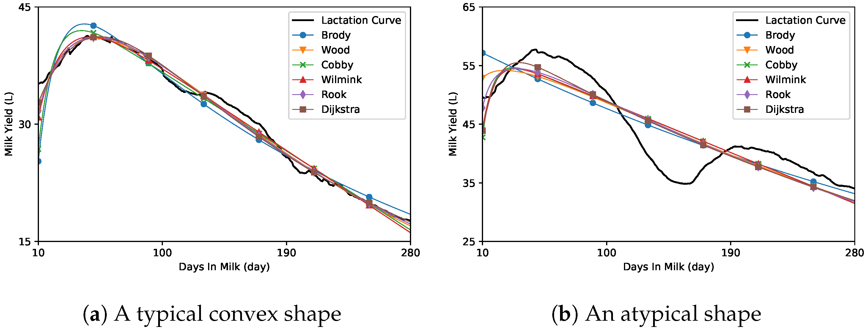
2.1. Conventional Regression Model
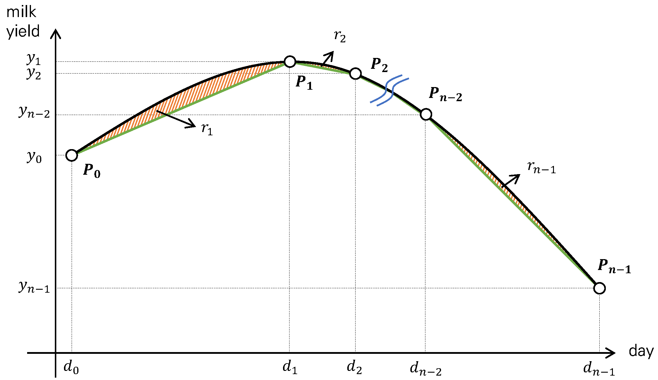
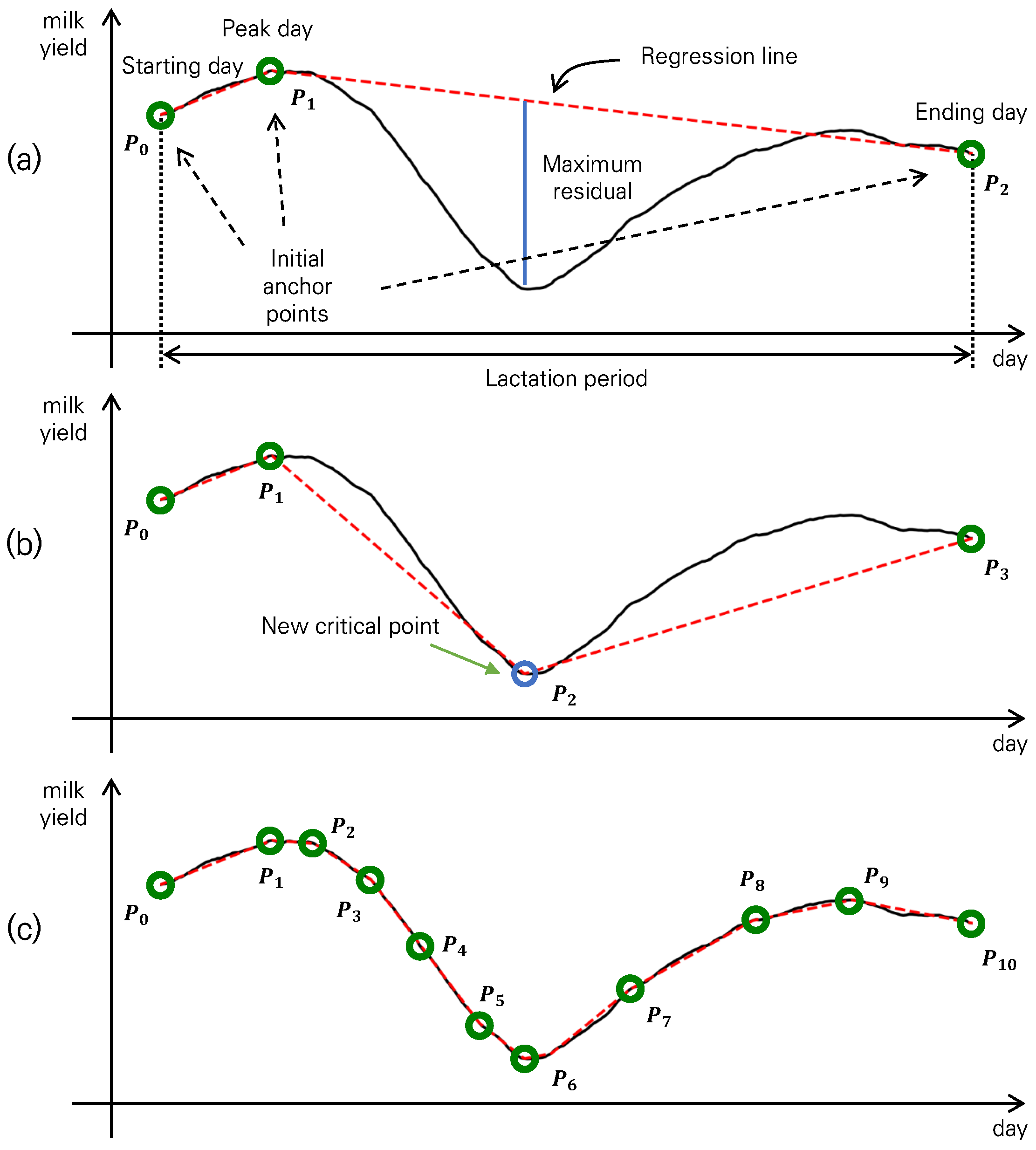
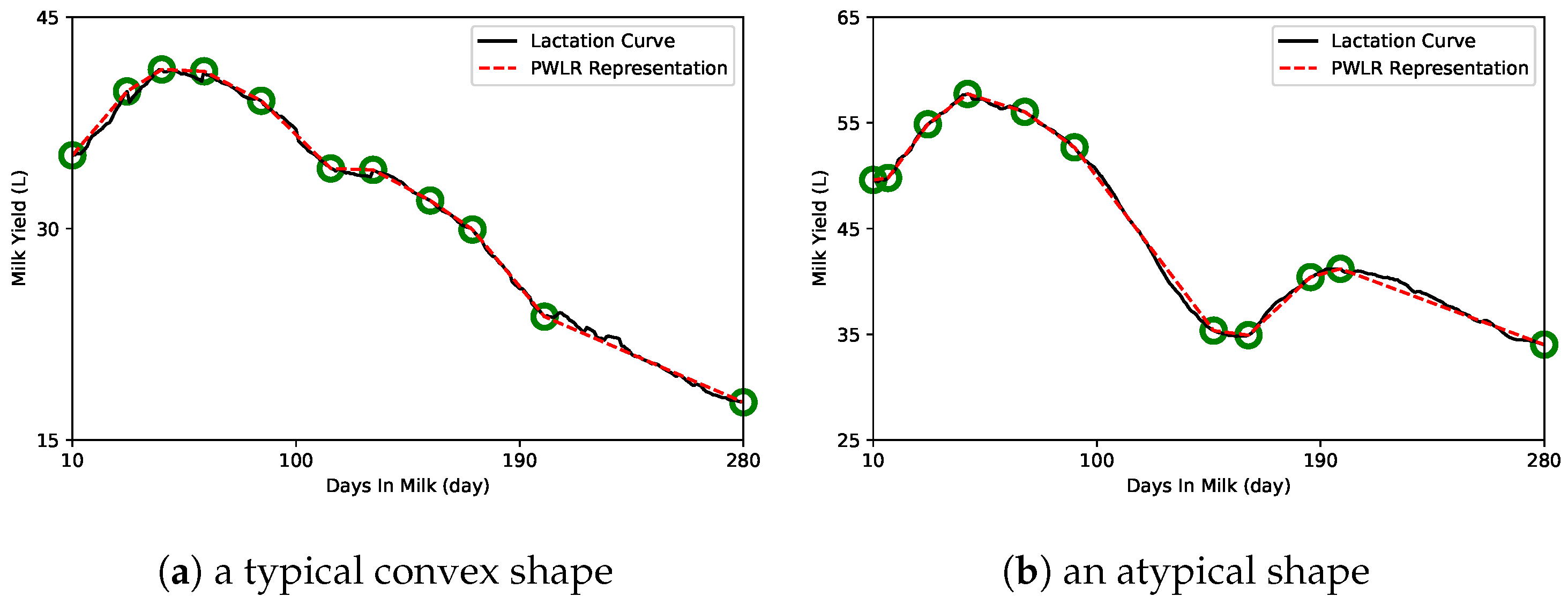
2.2. Piecewise Linear Regression Representation
2.3. Data Resources
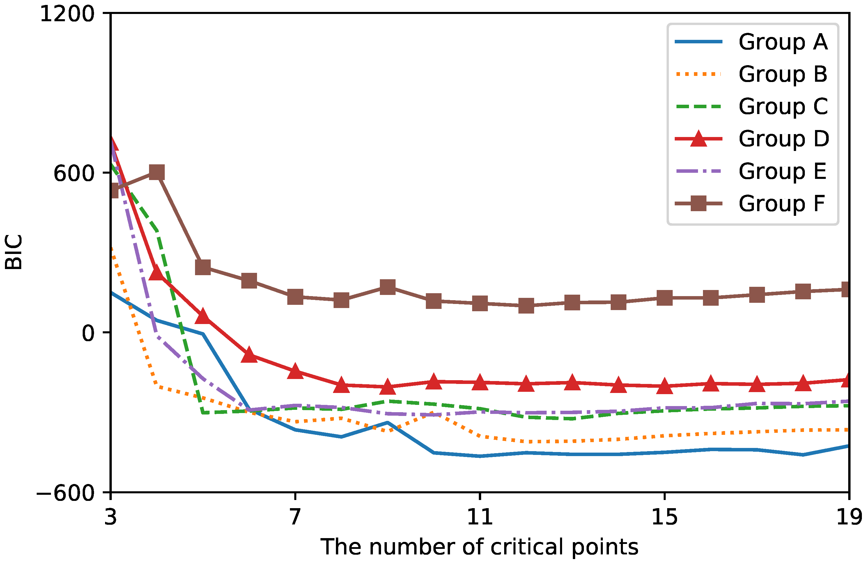
2.4. Evaluation
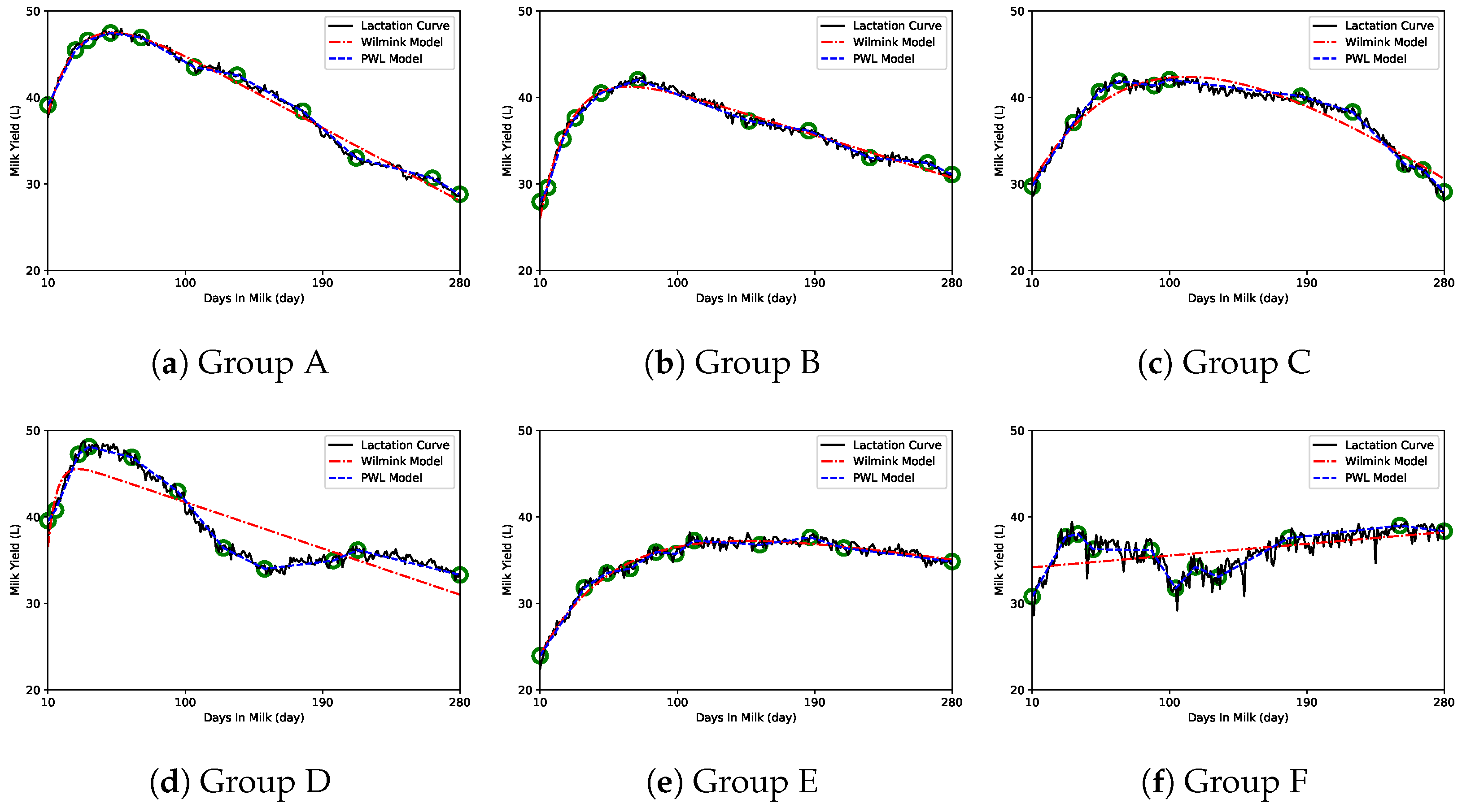
3. Results
4. Discussion
5. Conclusions
Author Contributions
Funding
Institutional Review Board Statement
Informed Consent Statement
Data Availability Statement
Acknowledgments
Conflicts of Interest
References
- de Noronha Figueiredo Vieira da Cunha, D.; Pereira, J.A.C.; Silva, F.F.e.; de Campos, O.F.; Braga, J.A.L.; Martuscello, J.A. Selection of models of lactation curves to use in milk production simulation systems. Rev. Bras. Zootec. 2010, 39, 891–902. [Google Scholar] [CrossRef] [Green Version]
- Dijkstra, J.; France, J.; Dhanoa, M.; Maas, J.; Hanigan, M.; Rook, A.; Beever, D. A Model to Describe Growth Patterns of the Mammary Gland During Pregnancy and Lactation. J. Dairy Sci. 1997, 80, 2340–2354. [Google Scholar] [CrossRef]
- Wood, P.D.P. Algebraic Model of the Lactation Curve in Cattle. Nature 1967, 216, 164–165. [Google Scholar] [CrossRef]
- Wilmink, J. Adjustment of test-day milk, fat and protein yield for age, season and stage of lactation. Livest. Prod. Sci. 1987, 16, 335–348. [Google Scholar] [CrossRef]
- Hossein-Zadeh, N.G. Application of nonlinear mathematical models to describe effect of twinning on the lactation curve features in Holstein cows. Res. Vet. Sci. 2019, 122, 111–117. [Google Scholar] [CrossRef]
- Rook, A.J.; France, J.; Dhanoa, M.S. On the mathematical description of lactation curves. J. Agric. Sci. 1993, 121, 97–102. [Google Scholar] [CrossRef]
- Lee, M.; Lee, S.; Park, J.; Seo, S. Clustering and Characterization of the Lactation Curves of Dairy Cows Using K-Medoids Clustering Algorithm. Animals 2020, 10, 1348. [Google Scholar] [CrossRef]
- Murphy, M.; Zhang, F.; Upton, J.; Shine, P.; Shalloo, L. A review of milk production forecasting models. In Dairy Farming: Operations Management, Animal Welfare and Milk Production; Global Agriculture, Nova Science Publishers: New York, NY, USA, 2018; pp. 14–61. [Google Scholar]
- Macciotta, N.P.; Dimauro, C.; Rassu, S.P.; Steri, R.; Pulina, G. The mathematical description of lactation curves in dairy cattle. Ital. J. Anim. Sci. 2011, 10, e51. [Google Scholar] [CrossRef] [Green Version]
- Iewdiukow, M.; Lema, O.; Velazco, J.; Quintans, G. Is it possible to accurately estimate lactation curve parameters in extensive beef production systems? Appl. Anim. Sci. 2020, 36, 509–514. [Google Scholar] [CrossRef]
- Nixon, M.; Bohmanova, J.; Jamrozik, J.; Schaeffer, L.; Hand, K.; Miglior, F. Genetic parameters of milking frequency and milk production traits in Canadian Holsteins milked by an automated milking system. J. Dairy Sci. 2009, 92, 3422–3430. [Google Scholar] [CrossRef]
- Grandl, F.; Furger, M.; Kreuzer, M.; Zehetmeier, M. Impact of longevity on greenhouse gas emissions and profitability of individual dairy cows analysed with different system boundaries. Animal 2019, 13, 198–208. [Google Scholar] [CrossRef] [PubMed]
- Masía, F.; Lyons, N.; Piccardi, M.; Balzarini, M.; Hovey, R.; Garcia, S. Modeling variability of the lactation curves of cows in automated milking systems. J. Dairy Sci. 2020, 103, 8189–8196. [Google Scholar] [CrossRef] [PubMed]
- Murphy, M.; O’Mahony, M.; Shalloo, L.; French, P.; Upton, J. Comparison of modelling techniques for milk-production forecasting. J. Dairy Sci. 2014, 97, 3352–3363. [Google Scholar] [CrossRef] [PubMed] [Green Version]
- Liseune, A.; Salamone, M.; Van den Poel, D.; van Ranst, B.; Hostens, M. Predicting the milk yield curve of dairy cows in the subsequent lactation period using deep learning. Comput. Electron. Agric. 2021, 180, 105904. [Google Scholar] [CrossRef]
- Brody, S.; Turner, C.W.; Ragsdale, A.C. The Relation between the initial rise and the subsquent decline of milk secretion following parturition. J. Gen. Physiol. 1924, 6, 541–545. [Google Scholar] [CrossRef]
- Cobby, J.M.; Le Du, Y.L.P. On fitting curves to lactation data. Anim. Sci. 1978, 26, 127–133. [Google Scholar] [CrossRef]
- Bouallegue, M.; M’Hamdi, N. Mathematical Modeling of Lactation Curves: A Review of Parametric Models. In Lactation in Farm Animals; M’Hamdi, N., Ed.; IntechOpen: Rijeka, Croatia, 2020; Chapter 6. [Google Scholar] [CrossRef] [Green Version]
- Vieth, E. Fitting piecewise linear regression functions to biological responses. J. Appl. Physiol. 1989, 67, 390–396. [Google Scholar] [CrossRef]
- Hamann, B.; Chen, J.L. Data point selection for piecewise linear curve approximation. Comput. Aided Geom. Des. 1994, 11, 289. [Google Scholar] [CrossRef] [Green Version]
- Hirotogu, A. Information Theory and an Extension of the Maximum Likelihood Principle. In Selected Papers of Hirotugu Akaike; Parzen, E., Tanabe, K., Kitagawa, G., Eds.; Springer: New York, NY, USA, 1998; pp. 199–213. [Google Scholar] [CrossRef]
- Schwarz, G. Estimating the Dimension of a Model. Ann. Statist. 1978, 6, 461–464. [Google Scholar] [CrossRef]
- Burnham, K.P.; Anderson, D.R. Multimodel Inference: Understanding AIC and BIC in Model Selection. Sociol. Methods Res. 2004, 33, 261–304. [Google Scholar] [CrossRef]
- Wit, E.; Heuvel, E.v.d.; Romeijn, J.W. ‘All models are wrong…’: An introduction to model uncertainty. Stat. Neerl. 2012, 66, 217–236. [Google Scholar] [CrossRef] [Green Version]
- Myung, I.J. The Importance of Complexity in Model Selection. J. Math. Psychol. 2000, 44, 190–204. [Google Scholar] [CrossRef] [Green Version]
- Browne, M.W. Cross-Validation Methods. J. Math. Psychol. 2000, 44, 108–132. [Google Scholar] [CrossRef] [PubMed] [Green Version]
- Liao, T.W. Clustering of time series data—A survey. Pattern Recognit. 2005, 38, 1857–1874. [Google Scholar] [CrossRef]
- Xu, D.; Tian, Y. A comprehensive survey of clustering algorithms. Ann. Data Sci. 2015, 2, 165–193. [Google Scholar] [CrossRef] [Green Version]
- Aghabozorgi, S.; Shirkhorshidi, A.S.; Wah, T.Y. Time-series clustering—A decade review. Inf. Syst. 2015, 53, 16–38. [Google Scholar] [CrossRef]
- Arthur, D.; Vassilvitskii, S. K-means++: The advantages of careful seeding. In Proceedings of the Eighteenth Annual ACM-SIAM Symposium on Discrete Algorithms, SODA ’07, New Orleans, LA, USA, 7–9 January 2007; Society for Industrial and Applied Mathematics: Philadelphia, PA, USA, 2007; pp. 1027–1035. [Google Scholar]
- Sölkner, J.; Fuchs, W. A comparison of different measures of persistency with special respect to variation of test-day milk yields. Livest. Prod. Sci. 1987, 16, 305–319. [Google Scholar] [CrossRef]
- Dekkers, J.; Ten Hag, J.; Weersink, A. Economic aspects of persistency of lactation in dairy cattle. Livest. Prod. Sci. 1998, 53, 237–252. [Google Scholar] [CrossRef]
- Western Canadian DHI Services. Lactation Curves. Available online: http://www.agromedia.ca/ADM_Articles/content/DHI_lactcrv.pdf (accessed on 20 January 2022).
- Thornley, J.H.; France, J. Mathematical Models in Agriculture: Quantitative Methods for the Plant, Animal and Ecological Sciences; CABI: Wallingford, UK, 2007. [Google Scholar] [CrossRef]
- Hickson, R.; Lopez-Villalobos, N.; Dalley, D.; Clark, D.; Holmes, C. Yields and Persistency of Lactation in Friesian and Jersey Cows Milked Once Daily. J. Dairy Sci. 2006, 89, 2017–2024. [Google Scholar] [CrossRef]
- Cole, J.; Null, D. Genetic evaluation of lactation persistency for five breeds of dairy cattle. J. Dairy Sci. 2009, 92, 2248–2258. [Google Scholar] [CrossRef] [Green Version]


| Model | Function for LC | |
|---|---|---|
| Brody (1924) | [16] | |
| Wood (1967) | [3] | |
| Cobby (1978) | [17] | |
| Wilmink (1987) | [4] | |
| Rook (1993) | [6] | |
| Dijkstra (1997) | [2] |
| Group | A | B | C | D | E | F |
|---|---|---|---|---|---|---|
| Number of cows | 119 | 64 | 50 | 47 | 38 | 12 |
| - distribution | 36.1% | 19.4% | 15.2% | 14.2% | 11.5% | 3.6% |
| - primiparous ratio | 14.3% | 43.8% | 36.0% | 21.3% | 73.7% | 83.3% |
| Parity | 2.61 | 2.16 | 2.30 | 2.57 | 1.63 | 1.25 |
| (0.12) † | (0.17) | (0.19) | (0.20) | (0.20) | (0.18) | |
| Total Milk Yield (liter/cow) | 10,713 | 9930 | 10,351 | 10,504 | 9509 | 9806 |
| (165) | (261) | (252) | (275) | (305) | (459) | |
| Peak Milk Yield (liter/cow) | 53.08 | 46.39 | 47.14 | 54.25 | 42.70 | 45.82 |
| (0.83) | (1.24) | (1.08) | (1.34) | (1.33) | (2.26) | |
| Peak Day (day) | 59.92 | 86.25 | 119.68 | 54.94 | 144.00 | 119.92 |
| (2.73) | (4.61) | (8.42) | (6.11) | (9.67) | (25.73) |
| V | Group A | Group B | Group C | ||||||
|---|---|---|---|---|---|---|---|---|---|
| 10 | 39.13 | 12.77 | 10 | 27.95 | 27.63 | 10 | 29.74 | 34.71 | |
| 28 | 45.49 | 5.94 | 15 | 29.59 | 2.62 | 37 | 37.10 | 10.19 | |
| 36 | 46.60 | 1.62 | 25 | 35.18 | 3.84 | 54 | 40.67 | 5.92 | |
| 51 | 47.46 | 3.83 | 33 | 37.64 | 1.91 | 67 | 41.90 | 4.58 | |
| 71 | 46.94 | 3.42 | 50 | 40.51 | 3.53 | 90 | 41.38 | 7.59 | |
| 106 | 43.52 | 8.32 | 74 | 42.05 | 6.03 | 100 | 42.07 | 2.90 | |
| 134 | 42.58 | 7.05 | 147 | 37.28 | 27.63 | 186 | 40.15 | 34.71 | |
| 177 | 38.41 | 9.05 | 186 | 36.16 | 9.63 | 220 | 38.33 | 10.18 | |
| 212 | 33.01 | 11.31 | 226 | 33.04 | 10.15 | 254 | 32.30 | 12.07 | |
| 262 | 30.66 | 12.77 | 264 | 32.44 | 9.72 | 266 | 31.63 | 4.86 | |
| 280 | 28.81 | 1.99 | 280 | 31.10 | 1.81 | 280 | 29.09 | 1.60 | |
| Group D | Group E | Group F | |||||||
| 10 | 39.53 | 22.03 | 10 | 23.93 | 22.40 | 10 | 30.77 | 47.19 | |
| 15 | 40.77 | 3.54 | 39 | 31.78 | 10.24 | 32 | 37.67 | 13.38 | |
| 30 | 47.21 | 8.63 | 54 | 33.50 | 4.61 | 40 | 38.00 | 7.74 | |
| 37 | 48.10 | 2.91 | 69 | 34.01 | 5.05 | 50 | 36.24 | 7.64 | |
| 65 | 46.87 | 14.92 | 86 | 35.91 | 6.02 | 88 | 36.12 | 32.69 | |
| 95 | 42.94 | 16.07 | 99 | 35.72 | 5.53 | 104 | 31.73 | 12.87 | |
| 125 | 36.38 | 15.30 | 111 | 37.24 | 4.81 | 117 | 34.19 | 11.03 | |
| 152 | 33.97 | 9.34 | 154 | 36.76 | 16.66 | 132 | 33.03 | 13.41 | |
| 197 | 34.92 | 18.58 | 187 | 37.61 | 10.16 | 178 | 37.52 | 33.21 | |
| 213 | 36.14 | 6.41 | 209 | 36.38 | 9.08 | 251 | 38.97 | 47.19 | |
| 280 | 33.27 | 22.03 | 280 | 34.81 | 22.40 | 280 | 38.32 | 10.07 | |
| LC | Group | Whole | |||||||
|---|---|---|---|---|---|---|---|---|---|
| Model | A | B | C | D | E | F | Mean | Set | |
| Brody | 2.553 | 0.788 | 2.073 | 2.682 | 1.261 | 2.019 | 1.896 | 0.742 | |
| Wood | 0.668 | 0.953 | 1.147 | 2.675 | 0.507 | 1.978 | 1.321 | 0.609 | |
| Cobby | 1.009 | 0.767 | 1.999 | 2.547 | 1.261 | 2.019 | 1.600 | 0.663 | |
| Wilmink | 0.668 | 0.524 | 1.006 | 2.546 | 0.551 | 1.881 | 1.196 | 0.244 * | |
| Rook | 0.635 | 0.600 | 1.053 | 2.563 | 0.524 | 1.881 | 1.209 | 0.313 | |
| Dijkstra | 0.693 | 0.464 | 1.121 | 2.368 | 0.578 | 2.018 | 1.207 | 0.248 | |
| PWLR | 0.338 * | 0.388 * | 0.470 * | 0.563 * | 0.459 * | 0.973 * | 0.532 * | 0.310 | |
| Brody | 4.400 | 3.559 | 4.214 | 5.010 | 3.395 | 4.302 | 4.147 | 4.176 | |
| (0.166) † | (0.184) | (0.185) | (0.244) | (0.213) | (0.527) | (0.253) | (0.093) | ||
| Wood | 3.887 | 3.431 | 3.896 | 5.040 | 3.166 | 4.245 | 3.944 | 3.894 | |
| (0.145) | (0.16) | (0.177) | (0.241) | (0.191) | (0.495) | (0.235) | (0.085) | ||
| Cobby | 4.033 | 3.390 | 4.178 | 5.052 | 3.351 | 4.303 | 4.051 | 4.007 | |
| (0.153) | (0.163) | (0.185) | (0.257) | (0.193) | (0.527) | (0.246) | (0.089) | ||
| Wilmink | 3.898 | 3.296 | 3.686 | 5.017 | 3.063 | 4.167 | 3.854 | 3.822 | |
| (0.154) | (0.163) | (0.168) | (0.255) | (0.188) | (0.499) | (0.238) | (0.089) | ||
| Rook | 3.812 | 3.328 | 3.809 | 4.958 | 3.095 | 4.178 | 3.863 | 3.812 | |
| (0.145) | (0.159) | (0.176) | (0.239) | (0.19) | (0.492) | (0.234) | (0.085) | ||
| Dijkstra | 3.760 | 3.253 | 3.717 | 4.846 | 3.045 | 4.148 | 3.795 | 3.741 | |
| (0.146) | (0.159) | (0.167) | (0.238) | (0.187) | (0.504) | (0.234) | (0.085) | ||
| PWLR | 2.721 * | 2.524 * | 2.898 * | 3.049 * | 2.479 * | 2.984 * | 2.776 * | 2.738 * | |
| (0.097) | (0.115) | (0.135) | (0.169) | (0.171) | (0.379) | (0.178) | (0.058) | ||
| LC | Group | Whole | |||||||
|---|---|---|---|---|---|---|---|---|---|
| Model | A | B | C | D | E | F | Mean | Set | |
| Brody | 4.436 | 3.956 | 4.068 | 4.605 | 3.709 | 7.460 | 4.289 | 4.524 | |
| Wood | 4.036 | 3.821 | 3.763 * | 4.682 | 3.486 * | 7.442 | 4.095 | 4.445 | |
| Cobby | 4.115 | 3.931 | 4.030 | 4.598 | 3.709 | 7.460 | 4.211 | 4.508 | |
| Wilmink | 4.035 | 3.787 | 3.780 | 4.601 | 3.513 | 7.210 | 4.075 | 4.429 | |
| Rook | 4.021 | 3.796 | 3.773 | 4.618 | 3.505 | 7.205 | 4.073 | 4.431 | |
| Dijkstra | 4.024 | 3.782 | 3.824 | 4.540 | 3.519 | 7.434 | 4.078 | 4.424 * | |
| PWLR | 3.987 * | 3.776 * | 3.765 | 4.141 * | 3.542 | 6.619 * | 3.952 * | 4.450 | |
Publisher’s Note: MDPI stays neutral with regard to jurisdictional claims in published maps and institutional affiliations. |
© 2022 by the authors. Licensee MDPI, Basel, Switzerland. This article is an open access article distributed under the terms and conditions of the Creative Commons Attribution (CC BY) license (https://creativecommons.org/licenses/by/4.0/).
Share and Cite
Lee, S.; Park, J. A Vector Representation of Lactation Curves for Dairy Cows. Agriculture 2022, 12, 395. https://doi.org/10.3390/agriculture12030395
Lee S, Park J. A Vector Representation of Lactation Curves for Dairy Cows. Agriculture. 2022; 12(3):395. https://doi.org/10.3390/agriculture12030395
Chicago/Turabian StyleLee, Seonghun, and Jaehwa Park. 2022. "A Vector Representation of Lactation Curves for Dairy Cows" Agriculture 12, no. 3: 395. https://doi.org/10.3390/agriculture12030395
APA StyleLee, S., & Park, J. (2022). A Vector Representation of Lactation Curves for Dairy Cows. Agriculture, 12(3), 395. https://doi.org/10.3390/agriculture12030395