Article

Simulating Cotton Growth and Productivity Using AquaCrop Model under Deficit Irrigation in a Semi-Arid Climate

by
Marjan Aziz
1,*,
Sultan Ahmad Rizvi
2,
Muhammad Sultan
3,*,
Muhammad Sultan Ali Bazmi
4,
Redmond R. Shamshiri
5,*,
Sobhy M. Ibrahim
6 and
Muhammad A. Imran
7
1
Department of Agricultural Engineering, Barani Agricultural Research Institute, Chakwal 48800, Pakistan
2
Water Conservation Division, Soil and Water Conservation Research Institute, Chakwal 48800, Pakistan
3
Department of Agricultural Engineering, Bahauddin Zakariya University, Bosan Road, Multan 60800, Pakistan
4
Department of Agronomy, Fodder Research Institute, Sargodha 40100, Pakistan
5
Department of Engineering for Crop Production, Leibniz Institute for Agricultural Engineering and Bioeconomy, 14469 Potsdam, Germany
6
Department of Biochemistry, College of Science, King Saud University, P.O. Box 2455, Riyadh 11451, Saudi Arabia
7
School of Environmental and Municipal Engineering, Xi’an University of Architecture and Technology, Shaanxi, Xi’an 710055, China
*
Authors to whom correspondence should be addressed.
Agriculture 2022, 12(2), 242; https://doi.org/10.3390/agriculture12020242
Submission received: 14 December 2021 / Revised: 27 January 2022 / Accepted: 1 February 2022 / Published: 8 February 2022
(This article belongs to the Special Issue Future of Irrigation in Agriculture)

Abstract

:
AquaCrop is a water-driven model that simulates the effect of environment and management on crop production under deficit irrigation. The model was calibrated and validated using three databases and four irrigation treatments (i.e., 100%ET, 80%ET, 70%ET, and 50%ET). Model performance was evaluated by simulating canopy cover (CC), biomass accumulation, and water productivity (WP). Statistics of root mean square error (RMSE) and Willmott’s index of agreement (d) showed that model predictions are suitable for non-stressed and moderate stressed conditions. The results showed that the simulated biomass and yield were consistent with the measured values with a coefficient of determination (R2) of 0.976 and 0.950, respectively. RMSE and d-index values for canopy cover (CC) were 2.67% to 4.47% and 0.991% to 0.998% and for biomass were 0.088 to 0.666 ton/ha and 0.991 to 0.999 ton/ha, respectively. Prediction of simulated and measured biomass and final yield was acceptable with deviation ˂10%. The overall value of R2 for WP in terms of yield was 0.943. Treatment with 80% ET consumed 20% less water than the treatment with 100%ET and resulted in high WP in terms of yield (0.6 kg/m3) and biomass (1.74 kg/m3), respectively. The deviations were in the range of −2% to 11% in yield and −2% to 4% in biomass. It was concluded that AquaCrop is a useful tool in predicting the productivity of cotton under different irrigation scenarios.

1. Introduction

The agriculture sector is integral to Pakistan’s economy. This sector contributes over 21% of GDP, absorbing 45% of the country’s total labor [1]. Cotton is one of the commercial cash crops of Punjab and Sindh in Pakistan [2]. The evaporative demand is high in semi-arid and arid areas of Indus Basin because of changing climatic conditions and rainfall patterns, which results in limiting agricultural productivity in the entire basin, except for the areas which receives plenty of water for agriculture. AquaCrop simulates in rainfed, deficit and full irrigation water regimes and predicts the achievable yields of the major crops. With the help of water driven function, AquaCrop calculates and converts the transpiration loss into biomass by using crop specific parameters [3,4]. AquCrop simulation using default cotton conservative parameters exhibited the best results [5]. Water productivity (WP) is a key element of agricultural water management in agricultural irrigated regions, and AquaCrop is a suitable tool to assess the water response to crop water productivity [6]. The maximum WP for wheat cultivar was found to be 1.54 kg/m3 that was acquired from 60% deficit irrigation [7,8]. Water being a precious commodity, could be saved by adapting water-saving techniques, which is only possible with proper assessment of water response to crop production [9]. Previous studies have demonstrated that AquaCrop accurately simulates the aboveground biomass and canopy cover of the crops under regular and deficit irrigation regimes [10,11,12,13]. As the world population increases, less water will be available for irrigation purposes in response t natural losses due to deep percolation, evaporation, and conveyance in furrow irrigation systems [14]. Drip irrigation uses less water than surface irrigation; thus, the irrigation water productivity is larger for drip systems in cotton production areas [15]. Rising water shortages [16,17] correlates the burden on agricultural productivity and sustainable increase in food demand [18]. AquaCrop model of the United Nations is simple, user friendly, and is practical for ultimate users such as extension workers, water managers, and professionals of irrigation organizations for planning purposes [19]. To evaluate how agricultural productivity will be affected by future shifts in water availability due to climate change, water production functions can be linked with crop models [8]. All other crop models are complicated, demanding advanced skills of calibration and operation as well as need a large number of parameters [20]. AquaCrop calibration is least demanding as compared to other crop models and has a limited number of key parameters to be adjusted. The model was originated from the yield response to water data and evolved to normalized water productivity. It was used to simulate crop productivity in multiple scenarios. The model was already parameterized for Gossypiumhirsutum for full irrigation (100% ET) and stressed (40%, 60%, and 80% of full 100% ET) irrigation levels for the Mediterranean environment of northern Syria [19]. Several climatic and agricultural procedure settings determined the optimal level of irrigation water applied for cotton production in southern Spain [19]. The AquaCrop model needs input data related to climate, soil, crop, irrigation, and initial soil water conditions [20]. Jin et al. [21] suggested that the AquaCrop model successfully predicted the canopy cover, biomass, and grain yield of winter wheat with high accuracy under different planting dates and irrigation environments. By drawing the water production function, the user can estimate the best water deficit level to obtain maximum yield. Keeping in view the water scarcity in the Pothwar area of Punjab, Pakistan, the AquaCrop model is planned to calibrate and revalidate for enhancing water productivity in the area. Thus, the main objective of the current study is to calibrate and validate the AquaCrop model (version 3.1) for full (100% ET) and stress or deficit (80%ET, 70% ET, and 50%ET) irrigation treatments for the semi-arid subtropical climate of Chakwal, Pakistan to find out the best optimal deficit irrigation level for cotton crop. The main features of the study model are to simulate canopy cover and biomass simulation and to draw water production functions.

2. Materials and Methods
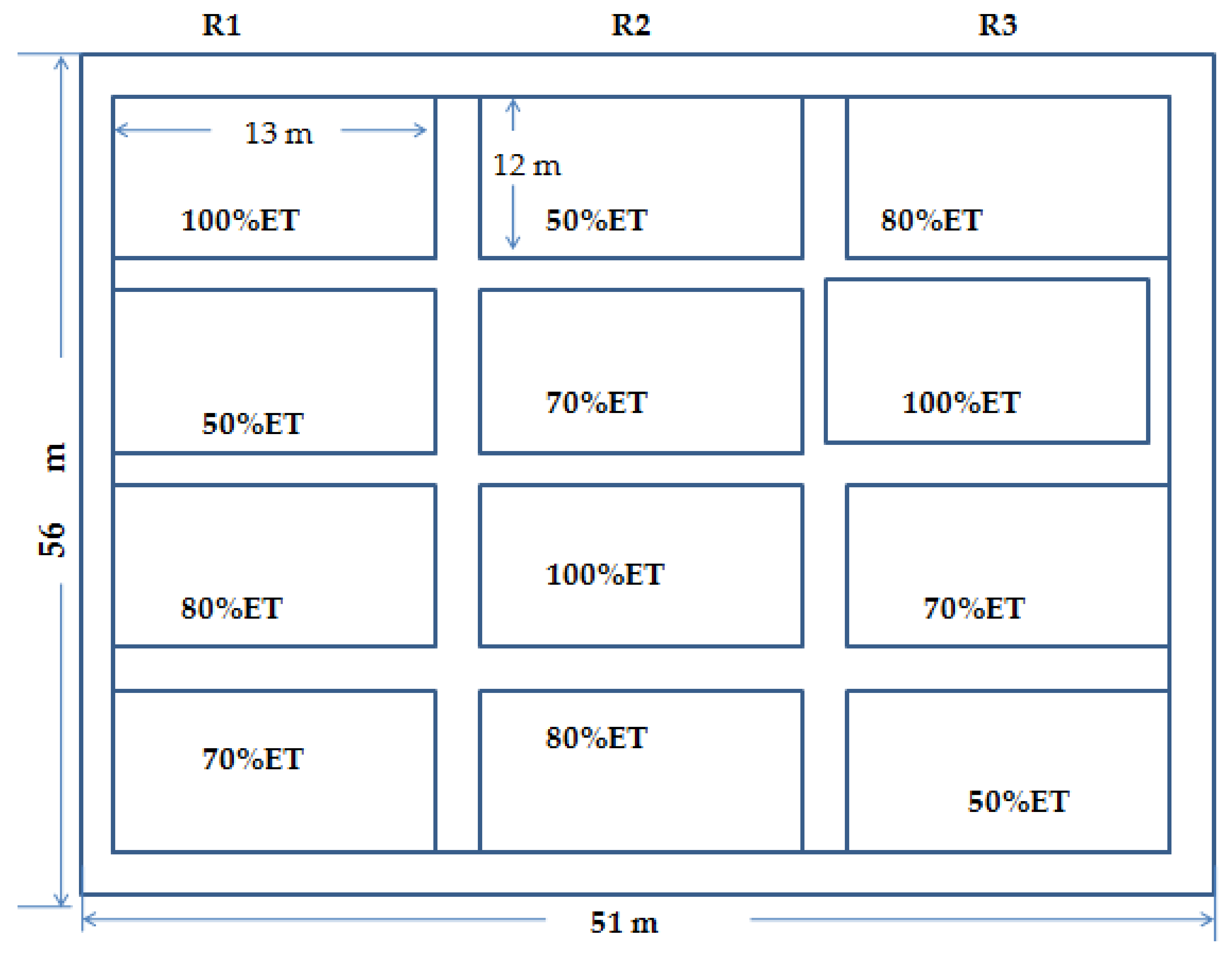
2.1. Research Area

The experiments were conducted at Barani Agricultural Research Institute, Chakwal, Punjab laying at 32°55’ N, 72°43’ E with 575 m altitude. The climate in the region is mainly semi-arid subtropical, with annual average rainfall is 350–500 mm. High-intensity rain showers are received during monsoon periods (July to September); the annual average rainfall for the period 1999–2017 was recorded as 235 mm.

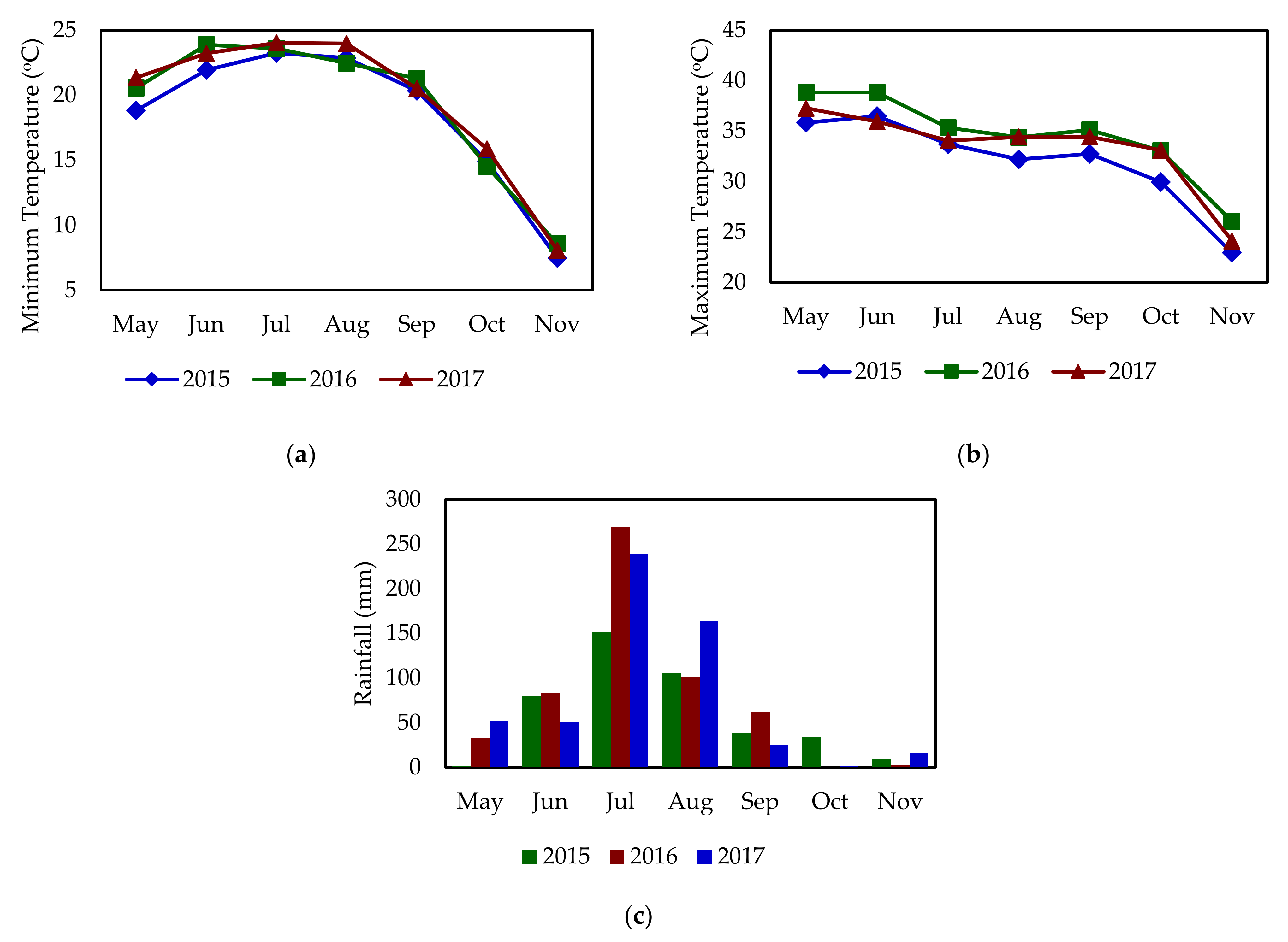
2.2. Weather and Soil Data

The weather data for the last 18 years (1999–2017) were collected from the nearby weather observatory of Soil and Water Conservation Research Institute (SAWCRI), Chakwal. This data was comprised of daily precipitation, daily maximum, and minimum air temperatures (Figure 1). FAO driven ETo calculator (http://www.fao.org/nr/water/eto.html (accessed on 10 November 2021)) [22] was used to calculate daily reference evapotranspiration (ETo). The calculator estimated the ETo from meteorological data of maximum, minimum temperature, solar radiation, wind speed and air humidity using FAO Penman-Monteith equation. Total rainfall of 291, 227, and 217 mm was received during the growing periods of 2015, 2016, and 2017, respectively (Figure 1). Normally, the driest month of the year was May, with an average humidity of around 30% (1999–2017). Soil characteristics of the experimental site were assessed by digging a pit (Figure 2) down to a depth of 1.2 m. The soil samples were collected from varying depths and analyzed in the laboratory, as given in Table 1. These soils were suitable for very distinct crops [23].
The soil water contents were measured with the help of a neutron moisture meter monitored with 7 days interval. Installed access tubes of poly vinyl chloride (PVC) in the field down to the depth of 1.3 m. The neutron probe was calibrated gravimetrically and developed the following two equations from calibration curves.
θv = 0.596 n − 0.122 For top-soil surface layer (R2 = 0.97)
θv = 0.331 n − 0.124 For subsurface soil layers (R2 = 0.98)
where θv = volumetric soil moisture content; n = count ratio, (observed counts/standard counts). Two calibration curves are required because the soil of the experimental area was sandy clay loam, the upper and deeper layer monitor the loss of neutron in surface and sub surface soil layers.

2.3. Field Management and Crop Data

The cotton (Gossypiumhirsutum) variety Desi was sown on 15 May 2015, 21 May 2016, and 15 May 2017, respectively, by keeping plant spacing of 0.7 × 0.45 m. The experimental plots were laid out in randomized complete block design (RCBD) with three replications (Figure 3). Four moisture levels of 100%ET, 80% ET, 70% ET, and 50% ET were maintained. The plot size was kept as 12 × 13 m (156 m2). The control treatment was kept at full water requirement of the plant (100% irrigation) throughout the growing season. Recommended doses of fertilizers were applied, i.e., nitrogen (114 kg/ha) in the form of urea (split doses giving a basal dose of 28 kg/ha at seed bed preparation while remaining quantity fertigated at alternative irrigations). Phosphorus was applied as basal dressing in the form of Tri super phosphate (TSP, 46% P2O5) at the rate of 125 kg/ha and potassium 62 kg/ha.
Data regarding canopy cover and aboveground biomass were recorded throughout the cropping season. Canopy cover was determined using ImageJ (Version 1.71) software. ImageJ measures canopy cover by digital images of the crop [24]. Cotton canopy images were acquired with the help of a Sony DKC-IDI digital camera with a spatial resolution of 786 × 561 pixels on a clear sunny day, when the sun was on peak (12:00–01:00 P.M) (Figure 4). With 10 days interval from the date after sowing (DAS). Only the two central rows of each plot were picturized. The final yield was taken at harvest. Statistical analysis was performed by using COSTAT software (www.softwaresea.com/Windows/download-CoStat-10243679.htm accessed on 15 May 2018) [25]. Treatment means of canopy cover, biomass, and yield were compared using DMR at a 5% significance level.
Three plants of cotton were randomly selected from each plot with an interval of 20 DAS and oven-dried at 105 °C for 24 h to obtain the aboveground biomass. The final yield of cotton was calculated from three samples of 2 m2 selected randomly and harvested from each plot once the cotton reached maturity.

2.4. Calibration of AquaCrop Model

AquaCrop was calibrated by using data of 2015, initially comparing the performance of 100%ET (full irrigation) for canopy cover (%) and biomass (ton/ha). The variables required for model calibration were explained specifically by the authors of [26,27] (Table 2) for each day of the simulation period.

2.5. Model Evaluation
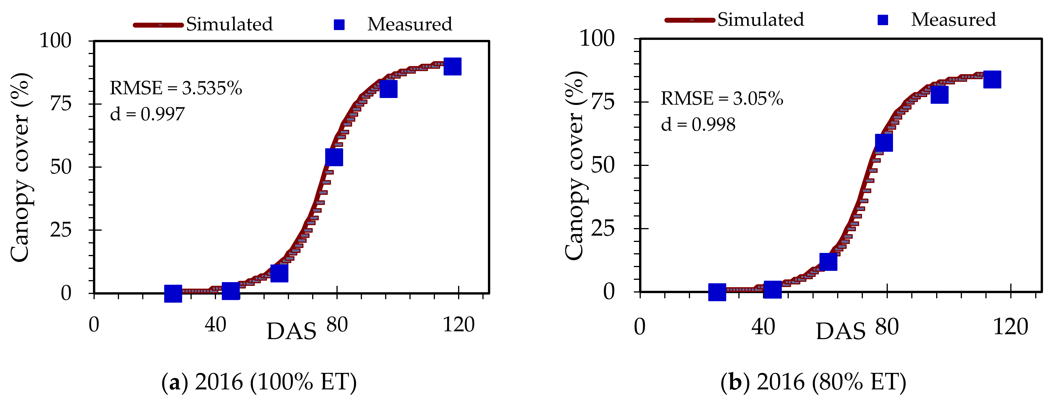
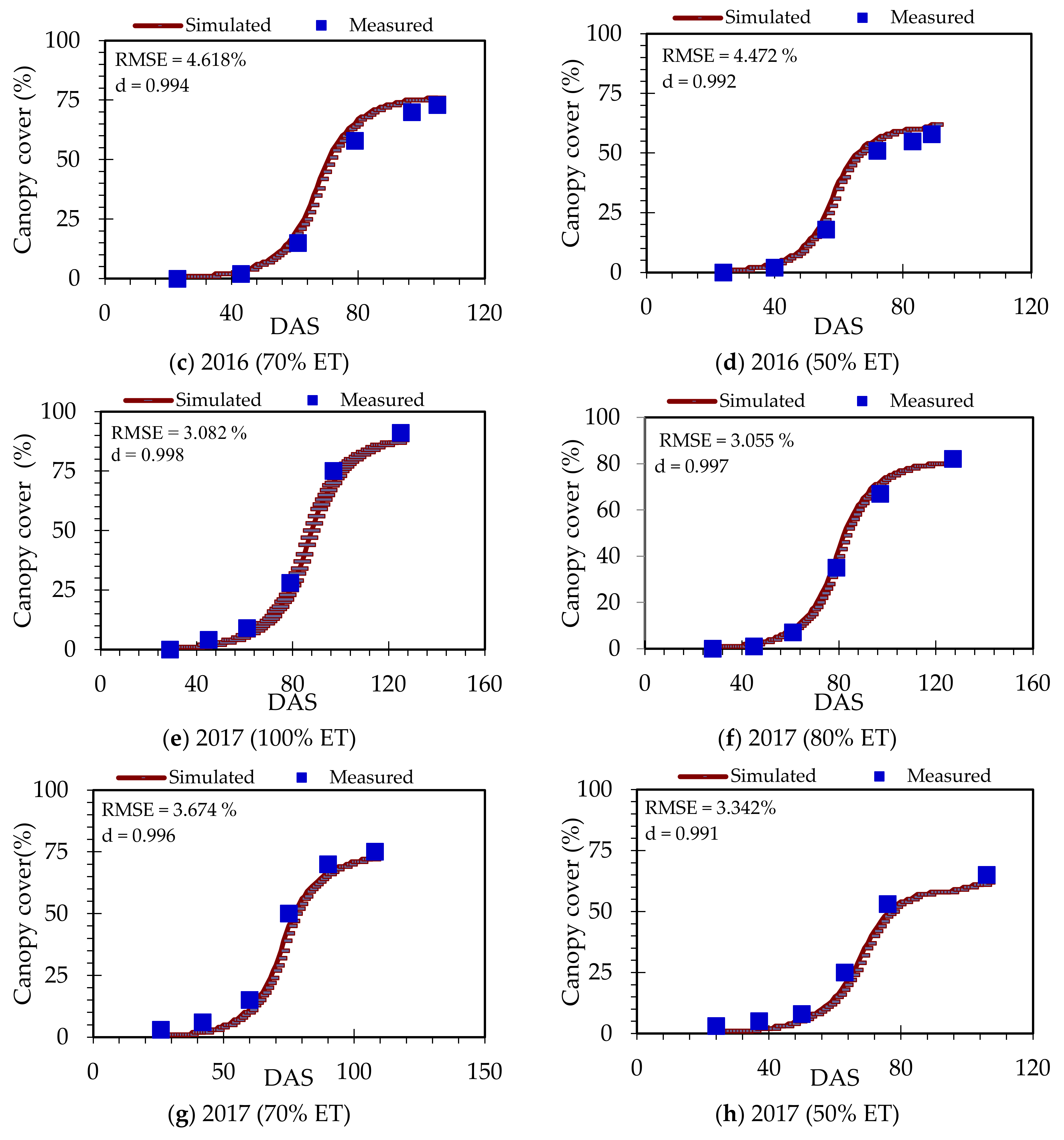
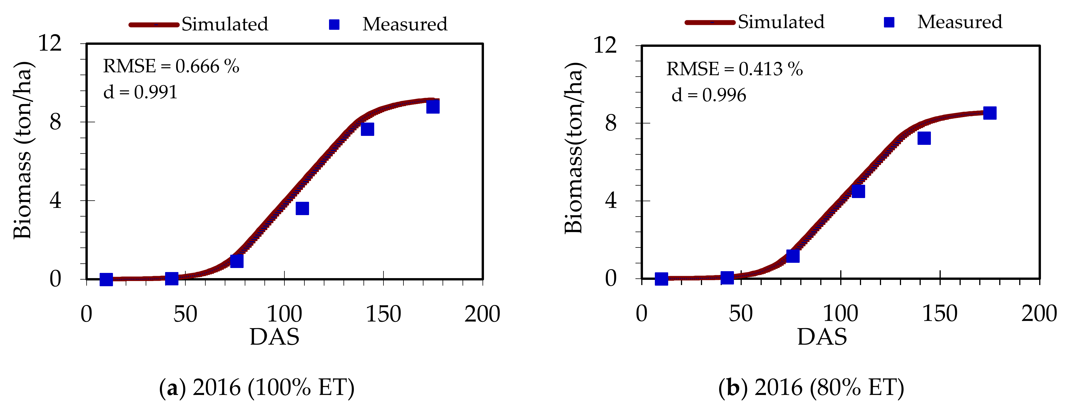
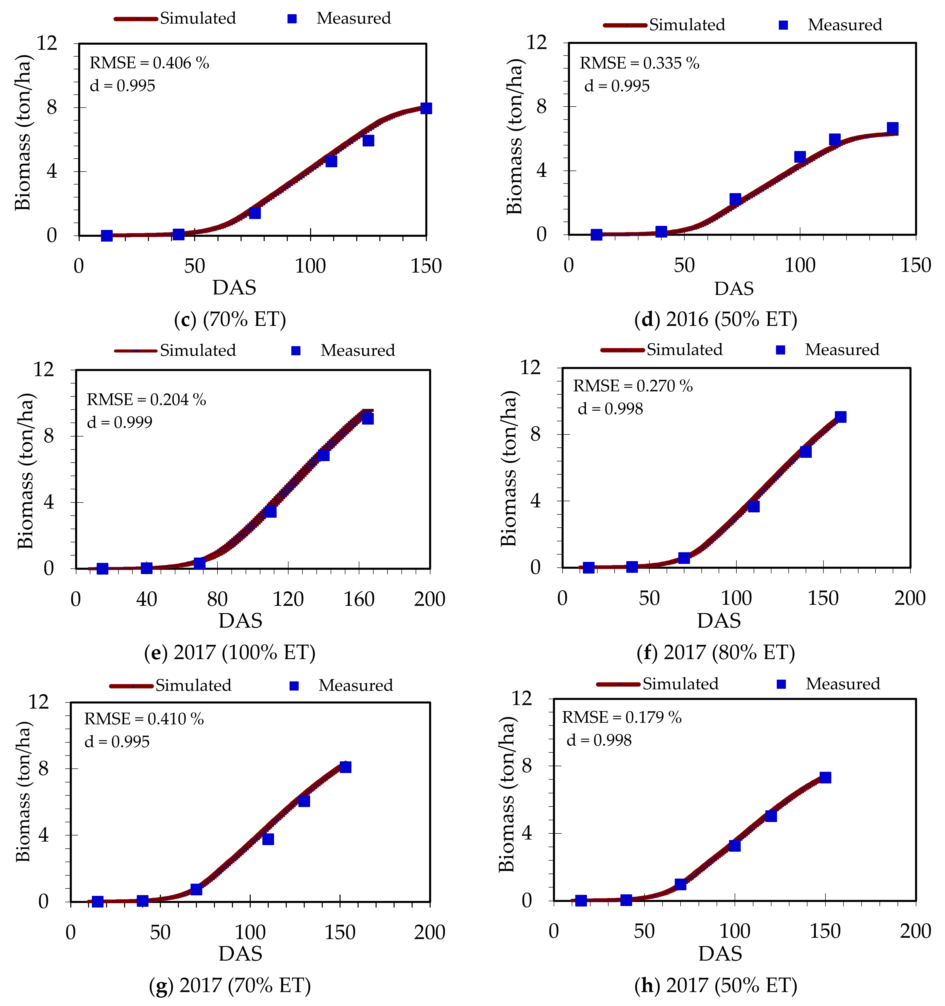
To evaluate the performance of AquaCrop, a straight line R2 value was calculated by plotting regression between the measured and simulated values of canopy cover (%), biomass (ton/ha), and yield (ton/ha), and correlation coefficients were determined. The subsequent statistics explicitly considered checking model goodness of fit: RMSE (root mean square error) and index of agreement (d) statistics [28]. The overall deviation in simulated and observed values are measured with the help of RMSE [29]. Index of agreement (d) is a measure of relative error in model estimates; it represents the degree to which simulated and observed values show similar deviations from the measured means [30]. When the value of RMSE approaches 0 and the value of d approaches 1, then the model shows perfect agreement.
R M S E = 1 N i = 1 N O i S i 2
where Oi = observed value; Si = simulated value; and N = no. of observations.
d = 1 i = 1 n P i O i 2 i = 1 n P i + | O i 2
where d = Willmott’s index of agreement, P’’= PiP; Pi = measured value; P = mean of measured value; O’= OiO; Oi = simulated value; and O = mean of simulated value.

3. Results

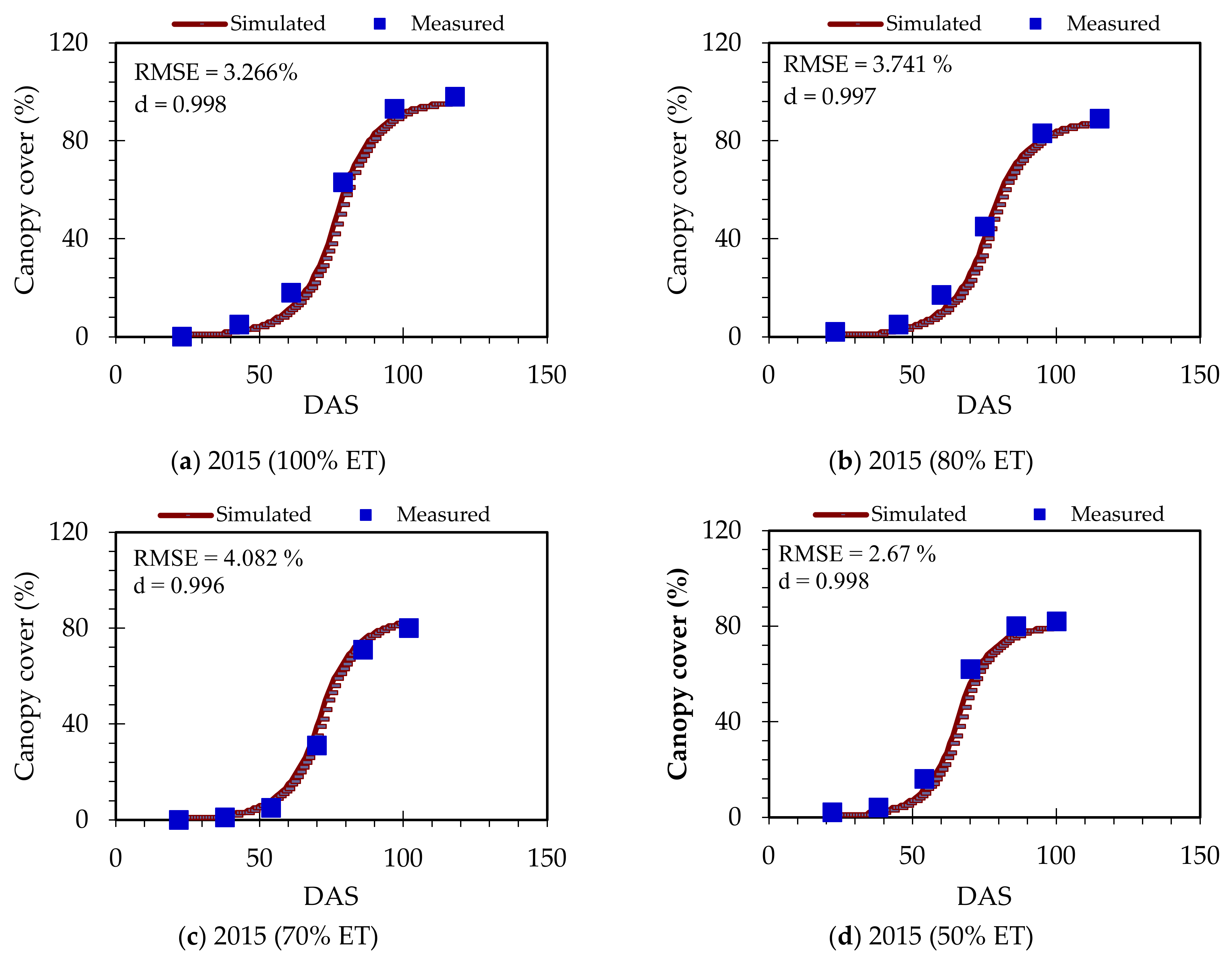
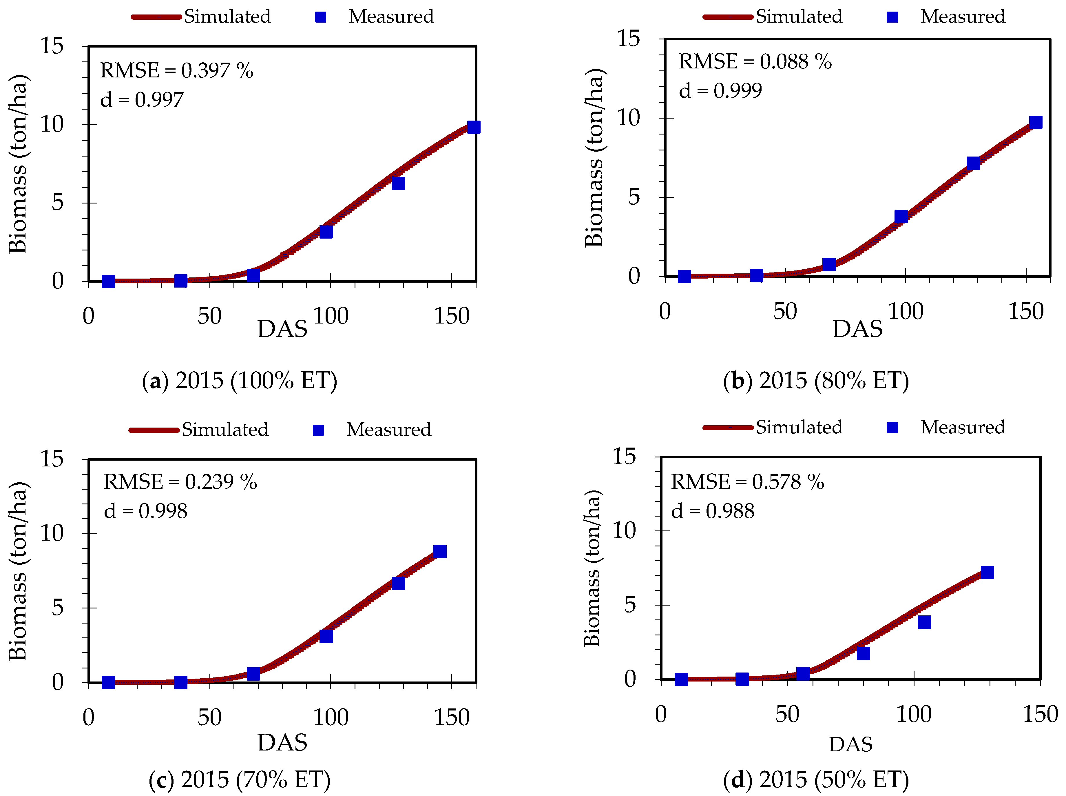
3.1. Model Calibration

AquaCrop was calibrated using the data set of 2015 (Table 2). The calibrated results revealed that the model was able to simulate canopy cover (CC) at different stages of crop growth (Figure 5). The values of RMSE were low and were considered suitable for model calibration.
The model showed an underestimation of the CC in the 100%ET irrigation treatment. The simulated maximum CC (%) was somewhat lower than the measured values (4% deviation). It could be possible due to the differentiation in initial moisture content between the simulated and measured values in deficit irrigation treatments. Strong agreement existed between measured and simulated canopy cover (Figure 5) for all the treatments. RMSE ranged from 2.670% to 4.082% and values of d-index from 0.996 to 0.998, respectively. Moreover, the results of low d-index value and high RMSE value in 70%ET. The values of the d-index clearly showed that the model predicted canopy cover very well in all irrigation treatments. The assessment of the model showed that the canopy cover of cotton simulated very well.
Figure 6 and Table 3 shows that AquaCrop simulated the aboveground biomass accurately for all irrigation treatments. Generally, there is a suitable fit between simulated and observed values of biomass by low RMSE and high d-index value (Figure 6). AquaCrop reasonably simulated the aboveground biomass for deficit treatments 80%ET and 70%ET (Table 3), as reflected by the statistical parameters. The highest value of RMSE was recorded in 50%ET treatment; the model showed an overestimation of biomass with a 4% deviation (Table 3). This treatment was observed to experience more water stress, an onset that began during the vegetative growth stage. As water stress increases, model robustness decreases. In the calibration process, canopy cover was underestimated, and biomass overestimated in 50%ET treatment. The overall model overestimates the biomass except for 80% ET treatment with 0 deviations (Table 3). The observed values of biomass were 9.837, 9.750, 8.785, and 7.201 ton/ha, while simulated values were 10.002, 9.729, 8.830, and 7.328 ton/ha for 100%ET, 80%ET, 70%ET, and 50% ET treatments, respectively (Table 3, Figure 7).

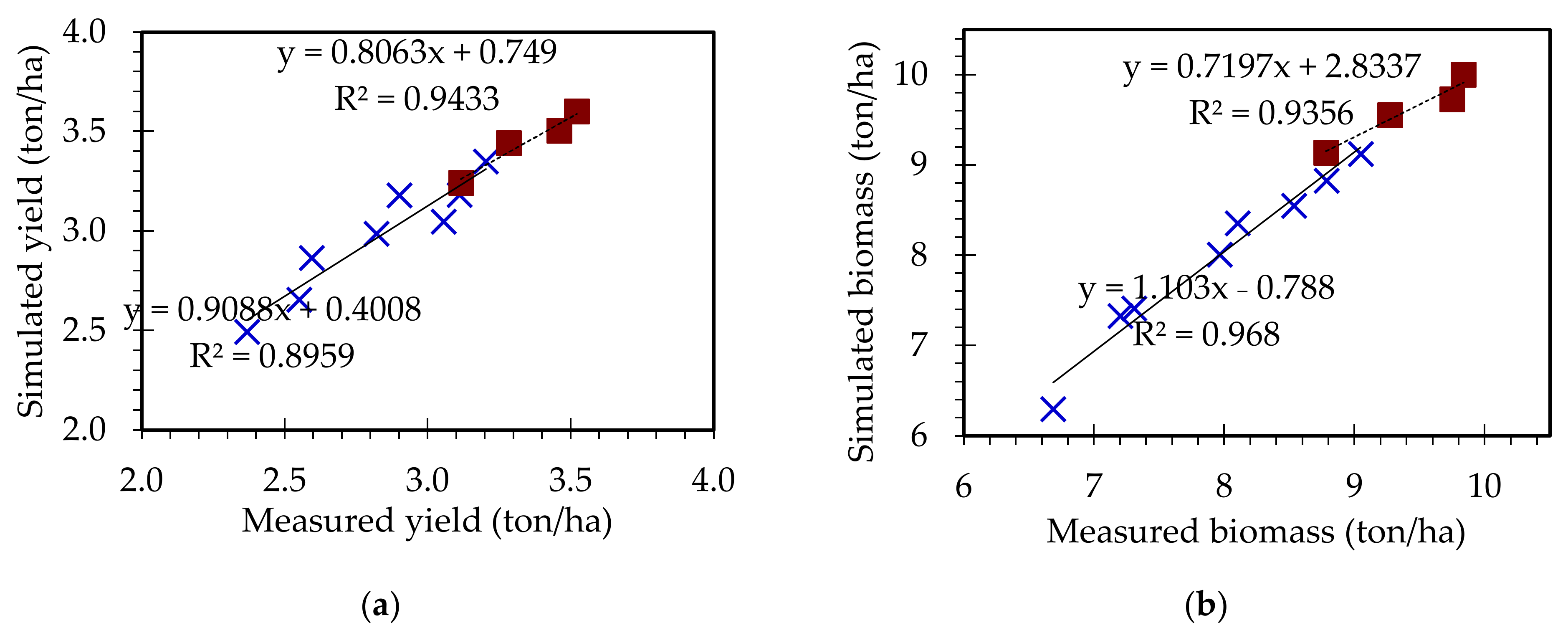
3.2. Model Validation

The calibrated parameters were used to validate AquaCrop for the years 2016 and 2017.The model favorably simulated the canopy cover development in 2016 and 2017 for all irrigation treatments. However, 50%ET in 2016 showed an overestimation of canopy cover (Figure 8d) with RMSE 4.472% and d-index value 0.992, but in 2017, 50%ET showed underestimation of canopy cover (Figure 8h) with RMSE 3.342%. The validation results of biomass are shown in Figure 9; accurate predictions of biomass were achieved for the years 2016 and 2017. The model over predicts the biomass, except for 50%ETwith RMSE = 0.335 to 0.179 % and d-index 0.995 to 0.998 for 2016 and 2017, respectively (Figure 9d,h). The results showed that performance of model was preferable (RMSE = 0.204% to 0.410%, d-index = 0.995 to 0.999) in 2017 as compared to 2016 (RMSE = 0.666% to 0.335%, d-index = 0.996 to 0.991) as depicted in Figure 9. AquaCrop predicted well aboveground biomass in 80%ET as compared to 100%ET in 2016 (Figure 9a,b) with RMSE = 0.413% and d-index = 0.996. Deficit irrigation treatments provided a suitable prediction of aboveground biomass for both years. RMSE values in 2017 were lower than all years because the model under predicted canopy cover in 2017.
For 2017 the observed values of biomass ranged from 7.308 to 9.271 ton/ha, while simulation values ranged from 7.413 to 9.556 ton/ha (Table 4). The deviations ranged from −6% to 4% between simulated and observed values for the cropping seasons of 2016 and 2017. An overall R2 value of 0.968 (validation database) was observed for the analysis of simulated and observed biomass for both years 2016 and 2017, Figure 7b, biomass was predicted with higher R2 value.
Lint yield measured for the year 2016 and 2017 were ranged from 2.367 to 3.116 ton/ha and 2.593 to 3.282 ton/ha, while simulated values were ranged from 2.493 to 3.24 ton/ha and 2.863 to 3.441 ton/ha, respectively, among treatments (Table 4). The difference in yield between 100%ET and 80%ET was small (no significant difference in yield) in 2015, 2016, and 2017 (Table 3 and Table 4). However, there was a significant difference in yield in 70%ET and 50%ET treatments. The model accuracy for yield prediction is shown in Figure 7a. The R2 value for yield was 0.895 between measured and simulated values using validation data bases, which verify that the model presents high accuracy in predicting yield.

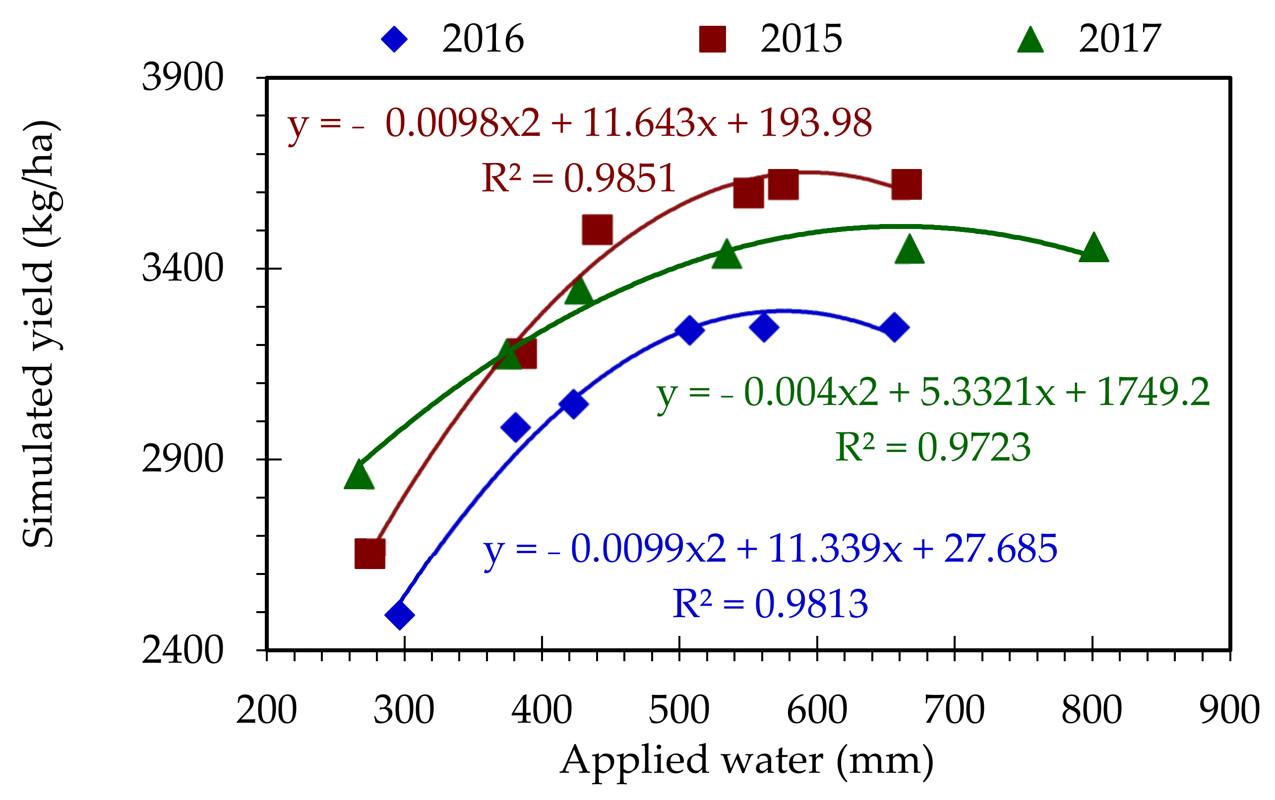
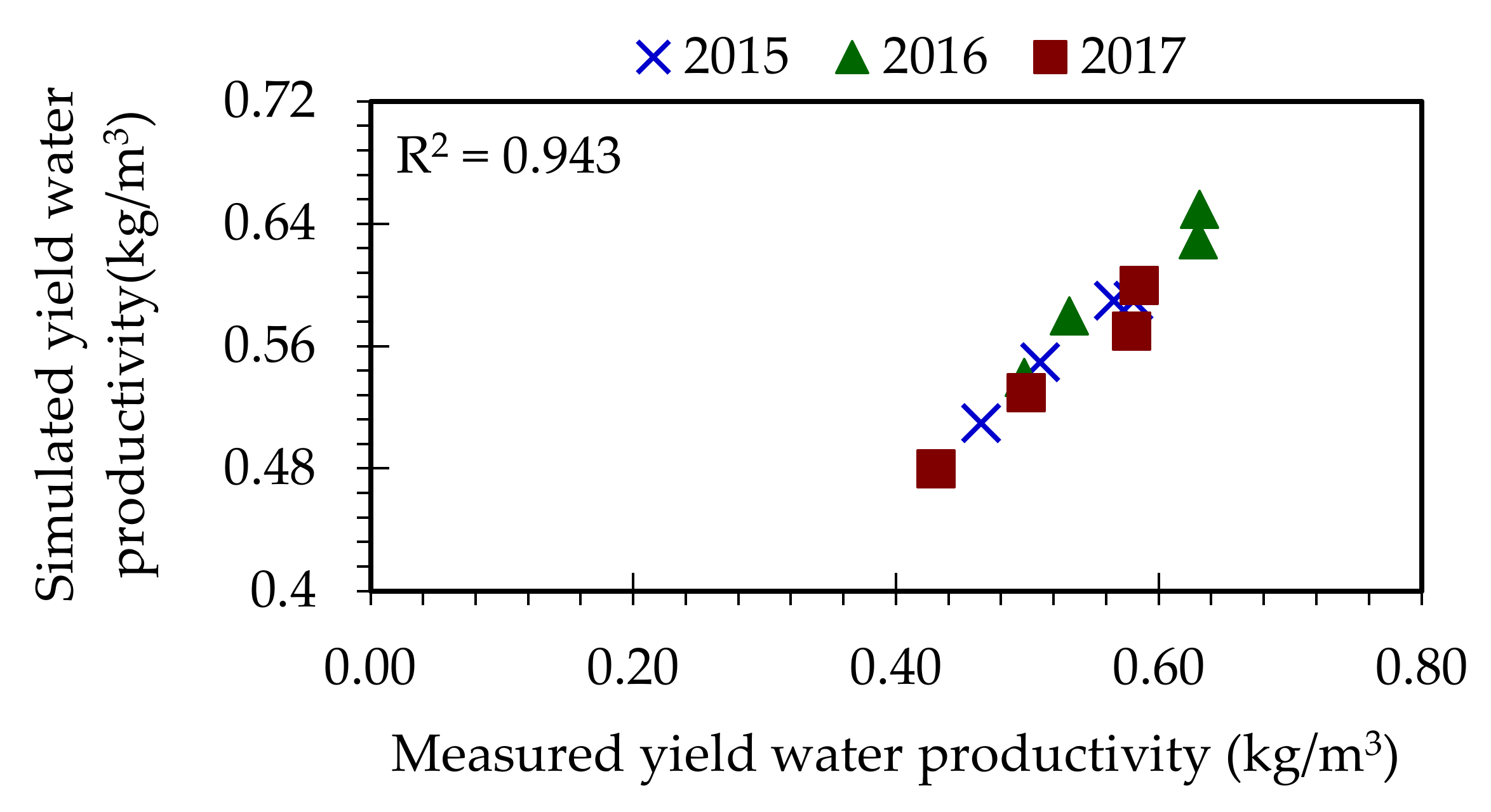
3.3. Water Productivity

The differences in the yield water productivity (YiWP) and biomass water productivity (BiWP) between measured and simulated values are shown in Table 5. Yield water productivity (YiWP) and biomass water productivity (BiWP) decreased with the increase in stress of water except 80%ET during all three years Figure 7a,b. In the present study, YiWP ranged from 0.43 to 0.63 kg/m3 reaching its maximum value of 0.63 kg/m3 in 2016 in 100% and 80% ET. Similarly, the value of BWP ranged from 1.44 to 1.79 kg/m3 reaching its maximum value of 1.79 kg/m3 in 2015 in 100% ET treatment. AquaCrop consistently overestimates the water use efficiencies, and due to water stress the deviations increased. The deviations were in the range of ₋2% to 11% in YiWP and ₋2% to 4% in BWP. The deviations were higher in YiWP as compared to BiWP; this is because the model also showed maximum deviation in the simulation of yield (Table 4). Maximum deviation was observed in YiWP of 50%ET treatment (10%, 9%, and 11% in 2015, 2016, and 2017, respectively). However, YiWP and BiWP were better in 80%ET both for calibration and validation databases (Table 5), indicating a potential for water saving. No significant difference was found in yield and biomass from 80%ET; thus, this treatment could be the best alternative to100%ET. The overall prediction of biomass water use efficiency in 2016 is better than that of 2015 and 2017. The linear regression between simulated and observed yield water productivity has the R2 value of 0.943 (Figure 10), suggesting that model prediction is fair.

4. Discussion

AquaCrop uses conservative parameters such as canopy cover, biomass, harvest index for simulation purposes. In the present study, AquaCrop simulated the canopy cover development and biomass accumulation of cotton for four irrigation treatments (100%ET, 80%ET, 70%ET, and 50% ET) and three databases (2015, 2016, and 2017). AquaCrop successfully predicted the canopy cover, biomass, and cotton lint yield. Suitable relationships were obtained among simulated canopy cover, biomass, yield, and water productivities (YiWP and BiWP) across three years under four treatments (Figure 5, Figure 6, Figure 7, Figure 8, Figure 9, Figure 10 and Figure 11, Table 3, Table 4 and Table 5). These results are in concurrence with that of the works of [11,31].
The model successfully predicted the lint yield of cotton with small deviations of 1% to 2%. Coefficient of variation R2 value of 0.943 and 0.935 (using calibration data set) were observed for the analysis of simulated and measured yield and biomass, respectively, indicating that model predicted yield and biomass very perfectly. However, there was a tendency to overestimate biomass in 2015. Figure 7a shows the accuracy of the model in predicting lint yield. A strong correlation was observed between the simulated and the measured values for the calibrated database (R2 = 0.943 and R2 = 0.935 for lint yield and biomass, respectively). The reduction in cotton yield mainly occurs when stress occurs in the reproductive stage of the crop. The most severely stressed treatment, 70% ET, and 50%ET in 2016, showed maximum deviation (10%) in yield between simulated and observed values. Simulated yield within 5% deviation shows the accuracy of AquaCrop in predicting yields, while the deviation values of 10% indicate that model accuracy declines in conditions of stressed water conditions. The same situations were reported by [32].
All irrigation treatments validated well the biomass (ton/ha) and canopy cover (%). The different climatic conditions in 2016 and 2017 lowered the yield; the reason might be the lower water productivity. AquaCrop provided suitable and adequate results of the biomass and canopy cover. The measured and simulated canopy cover used for validation AquaCrop model is shown in Figure 8 for the years 2016 and 2017, respectively. In general, simulation of canopy cover for the year 2017 showed the strongest agreement between simulated and observed values of canopy cover with lower RMSE (3.055% to 3.674%) and higher d-index values (0.991 to 0.998). The canopy cover simulation results were performed better in treatment of 80%ET (RMSE = 3.05%, d-index = 0.998 to 0.997) as compared to 100%ET (RMSE = 3.535% to 3.082%, d-index= 0.997 to 0.998) for both year 2016 and 2017 (Figure 8). It was concluded that to simulate canopy cover, biomass, and yield of cotton, AquaCrop model can be used. This research, as reported by the work of [12], suggested that climatic conditions, variety of crop, and irrigation practices can influence the performance of the AquaCrop model. The results showed that performance of model was better (RMSE = 0.204% to 0.410%, d-index = 0.995 to 0.999) in 2017 as compared to 2016 (RMSE = 0.666% to 0.335%, d-index = 0.996 to 0.991) which also depicted in Figure 9. AquaCrop predicted well aboveground biomass in 80%ET as compared to 100%ET in 2016 (Figure 9a,b) with RMSE = 0.413% and d-index = 0.996. The overview of some researchers is that AquaCrop model overestimates and underestimates the biomass and canopy cover, respectively, in the middle of the crop growth stage [33,34]. Similar results were obtained in the present study for all irrigation treatments. This could be possible due to the reason that AquaCrop clarifies the process of canopy cover decrease at crop senescence [35]. Biomass and yield water productivity decreases by the increase in transpiration amount in all four treatments. In the present study, the values of biomass water productivities were ranged from 1.44 to 1.79 kg/m3 in all growing seasons, and yield water productivity ranged from 0.43 to 0.63 kg/m3. These results are in agreement with the results reported in [36].
The model simulated canopy cover and biomass under different weather conditions with varying performance degrees. The year 2015 was the driest year, giving the lowest agreement between simulated and measured data. Severe water stress was observed during the early growth period of cotton in 2015 because the temperature was higher, and rainfall was less. Katerji et al. [37] reported that the level of plant water stress affected the model performance.
For quantification of the economic benefit of irrigations on average yield, it was required to calculate the estimated increase in yield as a function of increasing amounts of water delivered by the irrigation system. AquaCrop was run by changing the applied water values including water application at 150%ET, 120%ET, 100%ET, 80%ET, 70%ET, and 50%ET to verify the effect of increased and decreased irrigation water on the yield of cotton and keeping all the factors and data set constants. The simulated yield of cotton varied by changing applied water in three years (2015, 2016, and 2017). The plot showed that at a certain level, as depicted in Figure 11, yield decreased by increasing water applied for cotton.
There is a parabolic shape pattern achieved for water applied and simulated yield, which showed that cotton yield will be affected if water application increases from a certain safe level (Figure 11). The curve starts from a high slope, demonstrating that the production function is using water efficiently at low levels of irrigation. As the application of water level increases by 20%, the slope decreases. The slope of the parabolic line goes to zero as the water function attains maximum yield. AquaCrop works well for deficit irrigation, and if we increase water beyond 100%, then it will not change yield until and unless all crop parameters should be measured at that irrigation. Yield became stagnant after 100% ET, though we increased the amount of applied water (mm), 120%ET, and 150%ET, the last two points in three curves in Figure 8. The water production functions are curved lines, which change among climate scenarios. Using the quadratic formula, the best fit was observed; yield deficit and square of the available water deficit were varied proportionately. The regression lines fit very well with R2 ≥ 0.97 for the three functions. So, it indicated that AquaCrop worked well in water limiting conditions rather than in saturation. It predicts the impact of water stress on yield. In 2015 and 2017, yield versus water simulations, 80%ET showed better results, and there were no significant differences in yield in 100%ET and 80%ET treatments, but in 2016 there was a significant difference in yield in both treatments (100%ET and 80%ET). AquaCrop is stable and useful for different crops and environmental conditions. This study was conducted on cotton crops; however, other crops can also be studied.

5. Conclusions

Canopy cover, above ground biomass, lint yield and water productivity terms of grain yield and biomass of cotton were calibrated and validated by using AquaCrop model under four irrigation treatments. From the results of the present study, it was concluded that AquaCrop demonstrated its capability in simulating canopy cover, grain, and biomass yield to the reasonably suitable accuracy (d = 0.997 and 0.998, RMSE = 0.397% and 3.266%, for canopy cover and biomass, respectively). RMSE and d-index statistics were used for canopy cover (CC) for validation database were 2.67% to 4.47% and 0.991% to 0.998%, and for biomass were 0.088% to 0.666% and 0.991% to 0.999% for 2016 and 2017, respectively. Yield and biomass water productivity was found maximum in 80%ET, and there was no significant difference of yield in 100%ET and 80%ET, which indicated that the regions with a low delta of water will have yield loss. Model accuracy correlated (R2 = 0.95 and 0.97) between final measured and simulated yield and biomass, respectively. Thus, it is concluded that this model can be used as a decision-making tool for effective irrigation management practices.

Author Contributions

Conceptualization, M.A.; methodology, M.A. and R.R.S.; software, M.A., M.S.A.B. and M.A.I.; validation, M.A.I.; formal analysis, M.A., S.A.R. and M.A.I.; investigation, M.A., S.A.R., M.S. and R.R.S.; resources, M.S.; data curation, M.A., R.R.S. and M.A.I.; writing—original draft preparation, M.A.; writing—review and editing, M.S., M.S.A.B., R.R.S. and S.M.I.; visualization, S.A.R., M.S., M.S.A.B. and S.M.I.; supervision, M.A.; project administration, S.M.I.; funding acquisition, M.S., R.R.S. and S.M.I. All authors have read and agreed to the published version of the manuscript.

Funding

This work was supported by Researchers Supporting Project number (RSP-2021/100), King Saud University, Riyadh, Saudi Arabia.

Institutional Review Board Statement

Not applicable.

Informed Consent Statement

Not applicable.

Data Availability Statement

Data are contained within the article.

Acknowledgments

This work was supported by Researchers Supporting Project number (RSP-2021/100), King Saud University, Riyadh, Saudi Arabia. The authors acknowledge the financial support by the Open Access Publication Fund of the Leibniz Association, Germany.

Conflicts of Interest

The authors declare no conflict of interest.

References

  1. GoP. Economic Survey of Pakistan. 2018. Available online: http://finance.gov.pk/survey_0708.html (accessed on 14 November 2019).
  2. Howell, T.A. Enhancing water use efficiency in irrigated agriculture. Agron. J. 2001, 93, 281–289. [Google Scholar] [CrossRef] [Green Version]
  3. Steduto, P.; Hsiao, T.C.; Raes, D.; Fereres, E. AquaCrop—The FAO crop model to simulate yield response to water: I. Concepts and underlying principles. Agron. J. 2009, 101, 426–437. [Google Scholar]
  4. Mumtaz, H.; Farhan, M.; Amjad, M.; Riaz, F.; Kazim, A.H.; Sultan, M.; Farooq, M.; Mujtaba, M.A.; Hussain, I.; Imran, M. Biomass waste utilization for adsorbent preparation in CO2 capture and sustainable environment applications. Sustain. Energy Technol. Assess. 2021, 46, 101288. [Google Scholar]
  5. Tsakmakis, I.D.; Kokkos, N.P.; Gikas, G.D.; Pisinaras, V.; Hatzigiannakis, E.; Arampatzis, G.; Sylaios, G.K. Evaluation of AquaCrop model simulations of cotton growth under deficit irrigation with an emphasis on root growth and water extraction patterns. Agric. Water Manag. 2019, 213, 419–432. [Google Scholar]
  6. Jin, X.; Yang, G.; Li, Z.; Xu, X.; Wang, J.; Lan, Y. Estimation of water productivity in winter wheat using the AquaCrop model with field hyperspectral data. Precis. Agric. 2018, 19, 1–17. [Google Scholar]
  7. Salemi, H.R.; Salehi, M. Effects of limited irrigation on grain yield, yield Components and qualitative traits of some new wheat cultivars. Asian J. Plant Sci. 2005, 8, 74–77. [Google Scholar]
  8. Ashraf, M.N.; Mahmood, M.H.; Sultan, M.; Banaeian, N.; Usman, M.; Ibrahim, S.M. Investigation of Input and Output Energy for Wheat Production: A Comprehensive Study for Tehsil Mailsi (Pakistan). Sustainability 2020, 12, 6884. [Google Scholar] [CrossRef]
  9. Qureshi, A.S.; McCornick, P.G.; Qadir, M.; Aslam, Z. Managing salinity and waterlogging in the Indus Basin of Pakistan. Agric. Water Manag. 2008, 95, 1–10. [Google Scholar] [CrossRef]
  10. García-Vila, M.H.; Fereres, L.; Mateos, F.; Orgaz, F.; Steduto, P. Deficit irrigation optimization of cotton with AquaCrop. Agron. J. 2009, 101, 477–487. [Google Scholar]
  11. Farahani, H.J.; Izzi, G.; Oweis, T.Y. Parameterization and evaluation of the AquaCrop model for full and deficit irrigated cotton. Agron. J. 2009, 101, 469–476. [Google Scholar]
  12. Salemi, H.; Mohd-Soom, M.A.; Lee, T.S.; Mousavi, S.F.; Ganji, A.; Yusoff, M.K. Application of AquaCrop model in deficit irrigation management of Winter wheat in arid region. Afr. J. Agric. Res. 2011, 610, 2204–2215. [Google Scholar]
  13. Abedinpour, M.; Sarangi, A.; Rajput, T.; Singh, M.; Pathak, H.; Ahmad, T. Performance evaluation of AquaCrop model for maize crop in a semi-arid environment. Agric. Water Manag. 2012, 110, 55–66. [Google Scholar] [CrossRef]
  14. GoP. Economic Survey of Pakistan. 2019. Available online: http://finance.gov.pk/survey_0708.html (accessed on 24 March 2020).
  15. Hossain, M.A.; Hassan, M.S.; Ahmmed, S.; Islam, M.S. Solar pump irrigation system for green agriculture. Agric. Eng. Int. CIGR J. 2014, 16, 1–15. [Google Scholar]
  16. Askalany, A.; Ali, E.S.; Mohammed, R.H. A novel cycle for adsorption desalination system with two stages-ejector for higher water production and efficiency. Desalination 2020, 496, 114753. [Google Scholar] [CrossRef]
  17. Riaz, N.; Sultan, M.; Miyazaki, T.; Shahzad, M.W.; Farooq, M.; Sajjad, U.; Niaz, Y. A review of recent advances in adsorption desalination technologies. Int. Commun. Heat Mass Transf. 2021, 128, 105594. [Google Scholar] [CrossRef]
  18. Aziz, M.; Rizvi, S.A.; Iqbal, M.A.; Syed, S.; Ashraf, M.; Anwer, S.; Usman, M.; Tahir, N.; Khan, A.; Asghar, S. A Sustainable Irrigation System for Small Landholdings of Rainfed Punjab, Pakistan. Sustainability 2021, 13, 11178. [Google Scholar] [CrossRef]
  19. Babel, M.S.; Deb, P.; Soni, P. Performance evaluation of AquaCrop and DSSAT-CERES for maize under different irrigation and manure application rates in the Himalayan region of India. Agric. Res. 2019, 8, 207–217. [Google Scholar] [CrossRef]
  20. Raes, D.; Steduto, P.; Hsiao, T.C.; Fereres, E. AquaCrop—the FAO crop model to simulate yield response to water: II. Main algorithms and software description. Agron. J. 2009, 101, 438–447. [Google Scholar] [CrossRef] [Green Version]
  21. Jin, X.; Feng, H.; Zhu, X.; Li, Z.; Song, S.; Song, X. Assessment of the AquaCrop model for use in simulation of irrigated winter wheat canopy cover, biomass, and grain yield in the North China Plain. PLoS ONE 2014, 9, 1–11. [Google Scholar] [CrossRef]
  22. Allen, R.G.; Pereira, L.S.; Raes, D.; Smith, M. Crop evapotranspiration—Guidelines for computing crop water requirements—FAO Irrigation and drainage paper 56. Fao Rome 1998, 300, D05109. [Google Scholar]
  23. Neina, D. The role of soil pH in plant nutrition and soil remediation. Appl. Environ. Soil Sci. 2019, 2019, 1–9. [Google Scholar] [CrossRef]
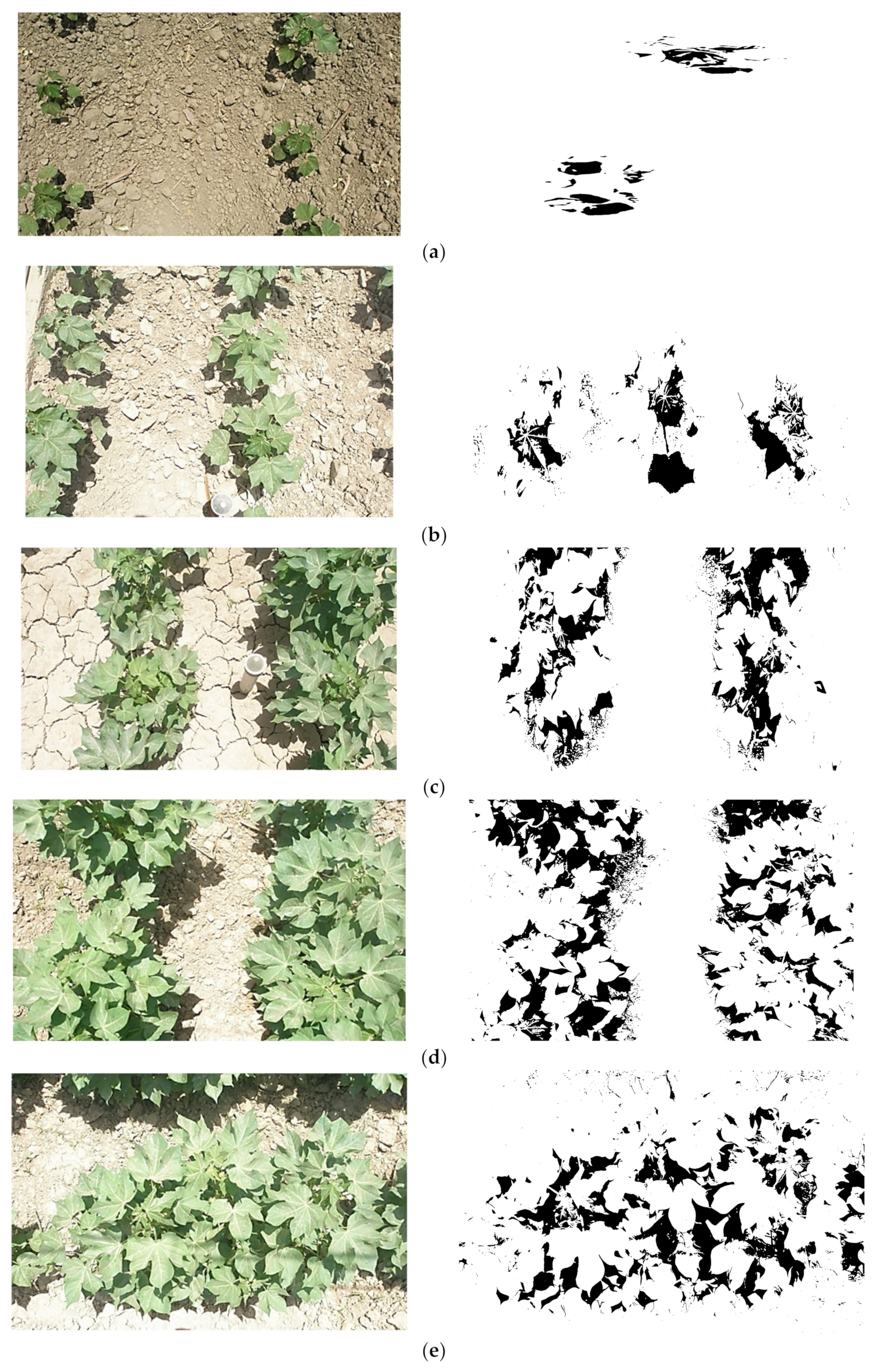
  24. Stewart, A.M.; Edmisten, K.L.; Wells, R.; Collins, G.D. Measuring canopy coverage with digital imaging. Commun. Soil Sci. Plant Anal. 2007, 38, 895–902. [Google Scholar] [CrossRef]
  25. Cardinali, A.; Nason, G. Costationarity of locally stationary time series using costat 55. J. Stat Soft. 2013, 55, 1–22. [Google Scholar] [CrossRef] [Green Version]
  26. Li, J.; Inanaga, S.; Li, Z.; Eneji, A.E. Optimizing irrigation scheduling for winter wheat in the North China Plain. Agric. Water Manag. 2005, 76, 8–23. [Google Scholar] [CrossRef]
  27. Giuliani, M.; Li, Y.; Castelletti, A.; Gandolfi, C. A coupled human-natural systems analysis of irrigated agriculture under changing climate. Water Resour. Res. 2016, 52, 6928–6947. [Google Scholar] [CrossRef]
  28. Loague, K.; Green, R.E. Statistical and graphical methods for evaluating solute transport models: Overview and application. J. Contam. Hydrol. 1991, 7, 51–73. [Google Scholar] [CrossRef]
  29. Greaves, G.E.; Wang, Y.-M. Assessment of FAO AquaCrop model for simulating maize growth and productivity under deficit irrigation in a tropical environment. Water 2016, 8, 557. [Google Scholar] [CrossRef]
  30. Zeleke, K.T.; Luckett, D.; Cowley, R. Calibration and testing of the FAO AquaCrop model for canola. Agron. J. 2011, 103, 1610–1618. [Google Scholar] [CrossRef]
  31. Evett, S.R.; Tolk, J.A. Introduction: Can water use efficiency be modeled well enough to impact crop management? Agron. J. 2009, 101, 423–425. [Google Scholar] [CrossRef]
  32. Asghar, N.; Akram, N.A.; Ameer, A.; Shahid, H.; Kausar, S.; Asghar, A.; Idrees, T.; Mumtaz, S.; Asfahan, H.M.; Sultan, M. Foliar-applied hydrogen peroxide and proline modulates growth, yield and biochemical attributes of wheat (Triticum aestivum L.) Under varied n and p levels. Fresenenius Environ. Bul. 2021, 30, 5445–5465. [Google Scholar]
  33. Heidarinia, M.; Naseri, A.; Broumandnasab, S.; Azari, A. Assessing AquaCrop model application in irrigation management innorth of Khosetan_Safiabad(CD). In Proceedings of the 1st National Water Management in Farm Conference, Karaj, Iran, 30–31 May 2012. [Google Scholar]
  34. Paredes, P.; Wei, Z.; Liu, Y.; Xu, D.; Xin, Y.; Zhang, B.; Pereira, L.S. Performance assessment of the FAO AquaCrop model for soil water, soil evaporation, biomass and yield of soybeans in North China Plain. Agric. Water Manag. 2015, 152, 57–71. [Google Scholar]
  35. Ahmadi, S.H.; Mosallaeepour, E.; Kamgar-Haghighi, A.A.; Sepaskhah, A.R. Modeling maize yield and soil water content with AquaCrop under full and deficit irrigation managements. Water Resour. Manag. 2015, 29, 2837–2853. [Google Scholar]
  36. Ahmad, H.S.; Imran, M.; Ahmad, F.; Rukh, S.; Ikram, R.M.; Rafique, H.M.; Iqbal, Z.; Alsahli, A.A.; Alyemeni, M.N.; Ali, S. Improving water use efficiency through reduced irrigation for sustainable cotton production. Sustainability 2021, 13, 4044. [Google Scholar]
  37. Katerji, N.; Campi, P.; Mastrorilli, M. Productivity, evapotranspiration, and water use efficiency of corn and tomato crops simulated by AquaCrop under contrasting water stress conditions in the Mediterranean region. Agric. Water Manag. 2013, 130, 14–26. [Google Scholar]
Figure 1. Monthly growing season weather data of (a) minimum temperature, (b) maximum temperature, and (c) rainfall (mm) (2015, 2016, and 2017).
Agriculture 12 00242 g001
Figure 2. (a) Soil pit to study soil properties from different depths of soil and (b) measurement of different depths.
Agriculture 12 00242 g002
Figure 3. The experimental layout of the study with four subsurface irrigation treatments.
Agriculture 12 00242 g003
Figure 4. Digital images of cotton plants. (a) Image of 20 DAS, (b) image of 40 DAS, (c) image of 50 DAS, (d) image of 60 DAS, and (e) image of 70 DAS.
Agriculture 12 00242 g004
Figure 5. Measured and simulated canopy cover under various irrigation treatments; (a) 100% ET, (b) 80% ET, (c) 70% ET, and (d) 50% ET.
Agriculture 12 00242 g005
Figure 6. Measured and simulated biomass ton/ha under various irrigation treatments (a) 100% ET, (b) 80% ET, (c) 70% ET, and (d) 50% ET for the year 2015.
Agriculture 12 00242 g006
Figure 7. Relationship between measured and simulated (a) lint yield and (b) biomass for the calibration (square) and validation databases (cross).
Agriculture 12 00242 g007
Figure 8. Validating results showing the comparison between measured and simulated values of canopy cover for the years 2016 (ad) and 2017 (eh).
Agriculture 12 00242 g008aAgriculture 12 00242 g008b
Figure 9. Validating results showing the comparison between measured and simulated values of biomass for the year 2016 (ad) and for the year 2017 (eh).
Agriculture 12 00242 g009aAgriculture 12 00242 g009b
Figure 10. Comparison between measured and simulated yield water productivity for three cropping seasons (2015, 2016, and 2017) under different water treatments.
Agriculture 12 00242 g010
Figure 11. Simulated cotton yield water functions obtained by varying the seasonal applied irrigation water.
Agriculture 12 00242 g011
Table 1. Soil characteristics of experimental field.
DepthTextureBulk
Density
KsatOrganic
Carbon
ClaySiltNitrogenFCpH in Water
(m)-(g/cm3)(mm/day)(%)(%)(%)(%)m3 m−3-
0–0.3Sandy loam1.520.750.456160.040.109.1
0.3–0.6Sandy loam1.70.60.351480.020.139.1
0.6–0.9Sandy loam1.60.80.26200.020.158.9
0.9–1.2Sandy loam1.390.830.028220.020.188.9
Ksat: saturated hydraulic conductivity; FC: field capacity.
Table 2. Main phenologic growth stages in days after sowing (DAS) and seasonal water applied for different treatments.
Agronomic DetailsGrowing Seasons
201520162017
Plant population (plants/ha)29,24027,24027,533
Date of sowing (DAS)15-May21-May15-May
Emergence (DAS)798
Flowering (DAS)555760
Senescence (DAS)121133135
Maturity (DAS)160175165
Maximum rooting depth (cm)102104102
Amount of irrigation water applied (m3/ha)
100%ET550050705340
80%ET440042304270
70%ET385038103740
50%ET275029702670
Table 3. Calibration results of biomass and lint yield for all four irrigation treatments for the year 2015.
TreatmentsVariablesMeasuredSimulatedDeviation (%)
100%ETBiomass (ton/ha)9.83710.0022
Yield (ton/ha)3.5213.62
80%ETBiomass (ton/ha)9.759.7290
Yield (ton/ha)3.463.5031
70%ETBiomass (ton/ha)8.7858.831
Yield (ton/ha)3.113.1792
50%ETBiomass (ton/ha)7.2017.3282
Yield (ton/ha)2.552.6544
Table 4. Validation results of biomass and lint yield for all four irrigation treatments for the year 2016 and 2017.
TreatmentsVariables20162017
MeasuredSimulatedDeviation (%)MeasuredSimulatedDeviation (%)
100% ETBiomass
(ton/ha)
8.789.13649.2719.5563
Yield
(ton/ha)
3.1163.2443.2823.4415
80% ETBiomass
(ton/ha)
8.5348.55109.0469.1261
Yield
(ton/ha)
3.0553.04603.2033.3474
70% ETBiomass
(ton/ha)
7.9638.00718.1028.3583
Yield
(ton/ha)
2.822.98562.9003.17710
50% ETBiomass
(ton/ha)
6.6856.298−67.3087.4131
Yield
(ton/ha)
2.3672.49352.5932.86310
Table 5. Comparison between measured and simulated water use efficiencies of three cropping seasons (2015, 2016, and 2017).
TreatmentsYield Water Productivity (YiWP) (kg/m3)Biomass Water Productivity (BiWP) (kg/m3)
Measured SimulatedDeviation (%)Measured SimulatedDeviation (%)
2015
100%ET0.570.5941.791.81
80%ET0.580.5921.781.833
70%ET0.510.5581.721.784
50%ET0.460.51101.581.655
2016
100%ET0.630.6531.751.792
80%ET0.630.6301.751.771
70%ET0.530.5891.671.723
50%ET0.500.5491.531.594
2017
100%ET0.580.57−21.681.71
80%ET0.590.631.691.65−2
70%ET0.500.5361.571.634
50%ET0.430.48111.441.54
Publisher’s Note: MDPI stays neutral with regard to jurisdictional claims in published maps and institutional affiliations.

