Assessing the Agricultural Sector’s Resilience to the 2008 Economic Crisis: The Case of Greece

Abstract

This paper studies the resilience of the agricultural sector compared to eight other sectors of the Greek economy. The analysis is based on a multilevel methodological framework aiming to integrate equilibrium and evolutionary approaches by incorporating temporal (recovery and adaptability), geographical (regional resilience), and sectorial (industrial resilience) aspects, quantified concerning the 2008 economic crisis. Within this composite context, resilience is measured on GVA data according to a dual-axis: horizontally, in terms of measuring the recovering time or the time of transition to a new state of functionality due to a shock, and vertically, in terms of capturing the variability caused by the shock, approximating the system’s adaptability. The analysis shows that the agricultural sector in Greece is generally resilient; although, it has not retained its pre-crisis maximum performance, and it has the smallest Gross Value Added magnitude and the most uneven distribution across the regional dimension. Overall, the analysis promotes the methodological conceptualization of regional resilience and provides insights into the case study of the structural analysis of the Greek rural economy.

1. Introduction

The agricultural sector in the European Union has (EU) faced various transformations in the context of the Common Agricultural Policy (CAP), which aims to improve the competitiveness of European agriculture in a globalized context. Toward the demand of competitiveness improvement, the agricultural sector must create value for producers, drive into the production of goods fulfilling the expectations of the customers, and contribute to the wider targets of the community, such as the livability of rural places and the preservation of the environment and the ecosystems [1,2,3,4]. Especially for the most developed countries, although it does not account for a large proportion of the Gross Domestic Product (GDP), the agricultural sector still comes with great direct and indirect benefits, both at the farm (microeconomic), and local and national (macroeconomic) levels [5]. A thriving agricultural sector also contributes to the social development of countries, as it ensures the supply of basic nutrients to the citizens and promotes the social cohesion targets by keeping the rural parts of countries alive [6,7,8,9]. Following its importance in the production set of the regional and national economies, the agricultural sector should be simultaneously stable, adaptive, and dynamic enough to ensure an active role towards regional and economic development [8,9,10,11]. This requirement interprets that the agricultural sector should be both equipped with quality structural (labor quality, specialization, high capital, level of technology, etc.) and functional (adaptability, self-organization, innovation, etc.) properties, to provide a major developmental factor in the complex configuration of the national and regional economy [12,13,14]. Within this context, recent research conceptualizing the complex setting of the modern economies [15,16,17,18,19], has brought into the light the new concept of economic resilience, which describes the capacity of an economic system to respond to shocks (disturbances), and withstand or recover or shift to a new state of functionality, if necessary, by undergoing adaptive changes to their structures and social and institutional arrangements [17]. Economic resilience is a complex concept consisting of diverse conceptualizations, such as geographical, structural or industrial, engineering, ecological, and dynamic, each expressing an aspect of complexity ruling an economic system. As current economic resilience enjoys fertile research, this paper tries to serve the demand of integrating diverse methodological aspects, and particularly to study the resilience of the agricultural sector in Greece to the 2008 economic crisis that considerably affected the dynamics of the national and regional economies of the country. Due to the complexity describing the framework of economic resilience, the paper has a double contribution: in methodological terms, it concerns studying economic resilience within an integrated context, by considering in common its industrial, regional (geographical), equilibrium, and evolutionary conceptual dimensions. This is undertaken by applying a multilevel analysis incorporating sectorial and regional divisions of the Greek economy and by comparing pre- and post-crisis performance about recovery time (to coordinate into an equilibrium rationale) and variability (to coordinate into an evolutionary rationale). The analysis builds on data of Gross Added Value and the Relative Workers Income. In empirical terms, the paper’s contribution regards providing a novel case study of the Greek agricultural sector’s resilience, which has not been previously studied for the country described by certain handicaps of the primary sector and a disproportional specialization in the tertiary sector.

2. Literature Review

▪

The conceptual framework of resilience

Although this concept of resilience has been previously used in various disciplines, such as physics (mechanics), ecology, biology, and psychology, it was just recently conceived in diverse aspects, grown, and broadly established within the context of regional science and economic geography [17]. This property is the so-called economic resilience [13,15,17,20], which, according to the authors of [17], is conceived as

“the capacity of a regional or local economy to withstand or recover from market, competitive, and environmental shocks to its developmental growth path, if necessary by undergoing adaptive changes to its economic structures and its social and institutional arrangements, to maintain or restore its previous developmental path, or transit to a new sustainable path characterized by a fuller and more productive use of its physical, human and environmental resources.”

In conceptual terms, resilience is composed of five main dimensions necessary to fully understand its complex nature, in any specific spatiotemporal context [17]: the shock (the origin of a disturbance), the system’s vulnerability (sensitivity to shocks), resistance (the initial economic impact of the shock), robustness (adaptability to shocks), and recoverability (the ability to recover into the initial conditions). In epistemological terms, economic resilience is mainly studied through a two-dimensional context [17,18], the equilibrium and evolutionary approaches, which, although are conceptually discrete, appear interrelated [18] within the context of the symbiotic relation describing a system’s structure (expressed in terms of multiplex equilibria) and functionality (expressed in temporal and evolutionary terms). In particular, equilibrium approaches conceive resilience either as an engineering process (engineering resilience), driving a system into a pre-existing equilibrium [13,19,20,21], or as an ecological process (ecological resilience), driving the system towards a new state of functionality [13,18,20]. On the other hand, evolutionary approaches conceive resilience within a dynamic context, as a property of continuous adaptation to ongoing changing conditions [13,17,18].

Within this context of polyphony [13,15,17,18,22], resilience is generally conceived as an intrinsic property of economic systems during their interaction with any (either internal or external) disturbances (shocks) and is defined within a complex context of its accompanying impacts, attributes, and determinants [13,17]. The authors of [18] note the importance of the shock’s time emergence for the definition and identification of resilience, driving into the configuration of two time periods (stages): the recession (or impact/downturn), and the recovery (or rebound/adaptation) phase. This conceptualization requires the specification of a meaningful “reference” period against which the impact of a shock can be measured, compared, and evaluated [17]. Moreover, proposing an interregional conceptualization, such as considering subnational differences in the study of resilience, is rather effective to drive better-targeted policies [18]. Toward this direction, the authors of [17] note that

“the notion of resilience is highly pertinent for analyzing how regions and localities react to and recover from shocks, and thence for understanding the role such shocks might play in shaping the spatial dynamics of economic growth and development over time.”

▪

Regional Resilience

The high compatibility of resilience in the regional and local economic research portfolio has caused an increasing interest in this concept of regional and urban science [17]. For instance, the authors of [23] examined the vulnerability and resilience of three coastal communities in the Solomon Islands, between January and May 2009, and found that social processes (community cohesion, good leadership, and individual support to collective action) were critical in influencing the perception that people had about their community’s ability to build resilience and cope with change. The work of [13] examined the resilience of seven municipalities of the southeast of Bahia (Brazil) to the cocoa crisis of the 1990s and showed that low land-use diversification makes the system low resilience. The authors of [24] examined the resilience of the EU regions to the 2008 economic crisis (period under consideration: 2008–2012) and found that the degree and nature of regional urbanization and specialization are important drivers of the resilience of EU regions. The work of [25] assessed the resilience of the Greek regions (NUTS 2) and prefectures (NUTS) to the 2008 economic crisis and found that metropolitan areas and regions based on manufacturing activities appeared more vulnerable compared to those with tourism specialization. The authors of [21] examined the role of cities as sources of regional resilience in Europe, for the period 1990–2011, and found that the quality of production, the level of external connectivity in cooperation networks, and the quality of urban infrastructure equipped cities and their hosting regions with greater economic resilience. The work of [26] examined the impact of the 2008 economic crisis on Greek urban economies (over the period 2011–2013), based on spatial econometric techniques applied to socio-economic, demographic, and policy variables configured at the municipal level. The authors found the impact heterogeneous, with the best pre-crisis performers (mainly urban-driven growth economies) being less resilient compared to lagging regions, and that domestic sectors (such as agriculture and tourism) contributed to the unemployment’s improvement. The work of [27] studied the determinants of firms’ resilience in the Eastern Europe’s regions during the period 2007–2011 based on employment change and found that firms of Eastern EU countries were more resilient, in terms of structural transformations, initial conditions, firms’ characteristics and capabilities, and spatial characteristics and irregularities of their broader environment. The authors of [28] examined the resilience of major UK regions to four major recessions of the past half-century (1974–76, 1979–83, 1990–93, and 2008–10), based on employment, and found, first, both continuities and significant changes in the regional impact of recession from one economic cycle to the next, and secondly that “region-specific” or “competitiveness” appeared to have played an equally, if not more, significant role on the resistance and recoverability of certain regions. The work of [29], using a 3D methodology applied (both on GDP and employment data) to selected European countries, examined regional economic resilience of European regions to several economic shocks since the early 1990s. The analysis highlighted that the 2008 economic crisis was not a single, but a series of closely connected events that amounted to a major economic shock. The authors of [30] studied, within an evolutionary framework, the capacity of European regions’ economies to develop new industrial specializations due to the 2008 economic crisis, on GDP data from the period 2004–2012. The analysis revealed diversity in the ability to develop new post-crisis industrial paths and introduced a typology of two resilience profiles, one describing regions that maintained medium/high entry levels after the shock (type A), and a second one describing regions that transited from low/medium entry levels to high entry levels after the shock (Type B). The work of [18] studied the impact and its underlying factors of the 2008 crisis on local labor markets, using econometric analysis, on annual data on pre- and post-crisis employment, and found a significant effect on regional resilience of the initial economic conditions, human capital, age structure, urbanization, and geography. The authors of [31] examined the resilience of British cities to the last four major economic shocks for the period 1971–2015 and found a distinct shift in the relation between resistance and recovery between these shocks, as well as major differences between northern and southern cities. Finally, the work of [22] examined the economic resilience of local industrial embeddedness of UK regions (NUTS2) to the 2008 financial crisis on data from the period 2000–2010, and found that embeddedness initially had a positive effect on resilience, whereas afterward it led to negative resilience effects.

▪

Structural (industrial or sectorial) resilience: the case of agriculture

The continuously increasing natural and environmental destructions, in conjunction with the worldwide economic crisis, highlight the importance of resilience within the context of the regional economy, where various conceptual components such as the demographic composition of the population, regional policy and governance, and the sector-based structure of the productivity system are taken into consideration [32]. As is evident, resilience builds on a rather complex conceptual framework, due to the complexity ruling the norms and other conditions describing the functionality of economic systems. Due to complexity, some conditions are definitive for the conceptual framework where resilience is studied. For instance, when the number of economic systems is plural and each system is considered as a segment of a broader unified market with certain geographical reference (regardless of the scale: international, national, regional, or lower), then resilience is studied within the framework of regional science and is conceived as regional resilience [17,20,21,25]. However, when a geographical subdivision is not available or does not matter as much as the economic performance of a system does, then resilience is conceived as economic resilience of the total system [17,18]. More specifically, in cases when the sectorial structure of an economic system is more important than the geographical aspect, then resilience is conceived as structural (or industrial or sectorial) resilience [9,17,33,34]; although, a geographical reference (usually at the national level, where sectorial information is by default available) is always included. Therefore, following the overall conceptualization of resilience [17,18], the sectorial resilience is a property describing the elasticity of an economic system’s industrial (or production) sector to respond to (either internal or external) disturbances (shocks), resulting in recovering (bounce-back) the pre-shocks or shifting to new states of functionality. The importance of sectorial resilience is related to the sectorial specialization of an economy, and the existence of a resilient sector may provide a pillar of economic growth and development in times of economic slumps [9,35]. Within the context that the development of a resilient agricultural sector is a default requirement of the EU and the ultimate goal of the CAP [1,2,3,4], a profound consideration of the agricultural resilience is crucial and calls for thorough research, despite the limited (compared to what is expected according to the basic importance of the agricultural goods) sector’s contribution to the GDP. This is because agriculture is by default a fundamental sector coming with great direct and indirect microeconomic and macroeconomic benefits for all economies [5].

Towards this requirement, several papers studied the resilience of the agricultural sector in times of economic recessions, either by examining the development trends of the reference sector or by comparing it with other economic sectors. The studies that evaluate the resilience of the agricultural sector on par with other sectors mainly rely on indicators of output, value, and employment [10,36,37,38,39]. For instance, at a subnational level, the authors of [40] investigated the resilience of rural, intermediate, and urban OECD regions in the 2008 economic crisis (for the periods 1995–2007 and 2007–2011), and found that rural remote and urban regions were more vulnerable than the intermediate and rural regions close to a city and that the capital metro regions had been hit harder by the crisis. At the national level, the work of [33] examined the economic resilience of the agricultural sector (including industries), on Lithuanian empirical data from the period 2004–2017, using a custom derivative indicator counting volatility of revenues, and found that the sector was increasing up to 2015 due to accession into the EU, whilst afterward the sector’s resilience showed an incline towards more profitable, but considerably more risky export markets. The authors of [34] examined the economic resilience of the agri-food sector in Mexico within a context of four conceptual dimensions: investments, vulnerability, product quality and information, and local economy, on data extracted from questionnaire-based research conducted in the context of the eighth Mexican rural census in 2007. The analysis, being an evaluation about the effectiveness of the current Mexican Agriculture, Livestock, and Forestry Census, provided insights into four areas of improvement for agricultural development policies, namely, profitability, market stability, safety networks, and product quality and information. From another perspective, the work of [41] examined the resilience of the agricultural sector in Zambia to drought and flood shocks, on data from the period 2010–2015, using a skew-normal regression approach. The analysis showed that economic diversification is a strategy to increase agricultural productivity and mitigate the adverse impact of droughts and floods on agricultural households. Next, the authors of [42] examined the economic resilience of Austrian agriculture during the period 1995–2019, by considering a selection of indicators of financial flexibility, stability in following the development path, diversification of activities, and diversification of export markets, and found that the agricultural sector in the country is quite resilient and forgiving of shocks. Finally, the authors of [9] studied the Lithuanian agricultural resilience within a three-dimensional context consisting of the production of food at affordable prices, assurance of farm viability, and provision of employment opportunities with a decent income for agricultural workers, on data from the period 2012–2019. The results showed that the overall level of Lithuanian agricultural resilience had declined, where the most evident negative changes were observed in the economic viability of farms, while the most robust levels related to the ability to provide local food at affordable prices.

▪

Measurement of resilience

As is evident by the previous short review, research in economic resilience is fruitful but simultaneously suffers from a high level of complexity [19,43,44] in terms of definition, modeling, and measurement. As the authors of [17] observe, “…yet there is no generally accepted methodology for how the concept should be operationalized and measured empirically…” and “…there is as yet no theory of regional economic resilience…”, “…and relatively little discussion of how the notion relates to other concepts such as uneven regional development, regional competitiveness, regional path dependence…”. For instance, engineering is typically measured by the speed of returning to equilibrium, whereas ecological resilience is by the force required before the structural characteristics of a system’s change become immanent [17,18]. For measuring resilience, [25] highlight the importance of capturing (i) changes due to a shock, ceteris paribus of the system’s structure and functionality; and (ii) the degree at which a system can create, sustain, or reorganize its capacity to learn and adapt. Towards an attempt of review, the authors of [17] observed that literature approaches measuring regional economic resilience can divide into four categories: (i) Case study based approaches, including mainly narrative studies of simple descriptive data, interviews with key actors, and interrogation of policies; (ii) Resilience indices, regarding singular, composite, and comparative measures of (relative) resistance and recovery, using key system variables of interest; (iii) Statistical time series models, which study the time evolution of the system and estimate the time duration for the shock’s impact to dissipate; and (iv) Causal structural models, which embed resilience in regional economic models, examining counterfactual scenarios of where the system would have been in the absence of a shock. Despite the methodology, some other dimensions also contribute to the observed diversity in the measuring of resilience [17,18], mainly concerning the configuration of the dataset on which resilience is computed. One dimension regards the time configuration of the shock, where the 2008 economic crisis enjoys most of the research interest [24,25,30]; although, there are some studies [28,29,31] that considered more than one past economic crises. Another dimension regards the time range of the examined period, varying from 1974–2015 [28], 1971 to 2015 [31], 2004–2012 [30], 1990–2015 [29], 2000–2010 [22], etc. A third dimension is the regional configuration of the system, which can be either international [24,40], national [25,28,31], regional [13], or even lower. Another dimension concerns the attribute of the dataset, measured in terms of various factors such as structural characteristics of the economy [23,26], GDP [20,21,24,29,30,40], GVA [31], employment [20,22,28,29], and demographic factors [25,45]. As the authors of [29] note, the attribute on which resilience is examined is determinative for the outcome of the study, and they demonstrated that the use of GDP compared to employment provided moderately different outcomes for regional economic resilience of European regions. The authors of [18] suggest using labor market data (employment, unemployment) than production output measures (GDP, GVA) due to their better availability and reliability at lower geographical levels, for which output measures calculation has been criticized. However, production outputs remain in the literature among the most popular variables for the measurement of resilience, along with employment and unemployment levels, and the modeling choices for an optimum approximation of resilience remain an open debate.

▪

Economic resilience and agriculture in Greece

Within the blossomed framework in the definition, measurement, and empirical research of this notion, the establishment of a resilient sector necessitates deep knowledge of the structural, functional, and geographical norms ruling the regional economic systems. This direction becomes particularly important for the agricultural sector, not only as an institutional requirement addressed by the EU’s policies, but also as a social demand towards the inequalities convergence and sustainable regional development [12,14]. Especially for the countries that lagged in the industrialization of their economy, the development of a resilient agricultural sector may become a pillar of stability towards regional development [14], since agriculture is immanent in the technological coefficients of many horizontal connections with other sectors [11], and therefore it determines the form and rate of economic development to a certain extent [12]. In Greece, the effort towards the country’s industrialization caused a fast decline of the agricultural sector and its contribution to the national economy [14,46]. In particular, while the agricultural specialization of Greece in 1950 counted 28% of the total GDP, its contribution shrunk in 3% in 2010 [46]. The structure of the Greek agricultural sector is generally poor because of the plethora of small and multi-fragmented farms, the low availability of irrigated agricultural land, and the disproportionally great active labor force of the sector [12], which for a considerable number (4 out of the 13) of regions in the country ranges between 20% and 30% of total regional employment [47]. In conjunction with the mixed mountainous and insular landscape, the inadequate infrastructure, the insufficient vocational training, the large percentage of aged farmers, and the ineffective trade of agricultural products, the Greek agricultural specialization is deficient compared to almost all other European and Mediterranean countries [12,14,46]. The regional specialization of the agricultural sector in the last decade in Greece ranges on average (95% confidence interval) from 11 to 14.5%, whereas for the secondary sector it is 16.5–24%, and for the tertiary sector it is 63.5–70% [14]. Moreover, the country has a considerable specialization in tourism, ranging from 15 to 20% of the Gross National Product [48]. In terms of resilience to the economic crisis, [25] applied pre- and after-crisis comparisons to a set of socio-demographic, economic, and welfare variables for the Greek regions, and found that regions specialized in tourism appeared more resistant, while metropolitan regions based on manufacturing appeared more vulnerable. On a further approach, the authors of [49] found that the recent 2008 economic crisis further intensified regional inequalities in Greece, by strengthening the prominent role of the Athens metropolitan region in the development map of the country and advancing regions with higher specialization in tradable and export-oriented sectors. As is evident by the previous information, the resilience profile of Greece seems to be more a matter of the disproportionally tertiary specialization, with an emphasis on tourism, of the country compared to the other production sectors. The overall geomorphological, infrastructure, and functional handicaps of the country, discriminate Greece as an interesting case study for the development of a resilient agricultural sector [12], toward the EU’s institutional requirements and the social demand into the inequalities convergence and sustainable regional development.

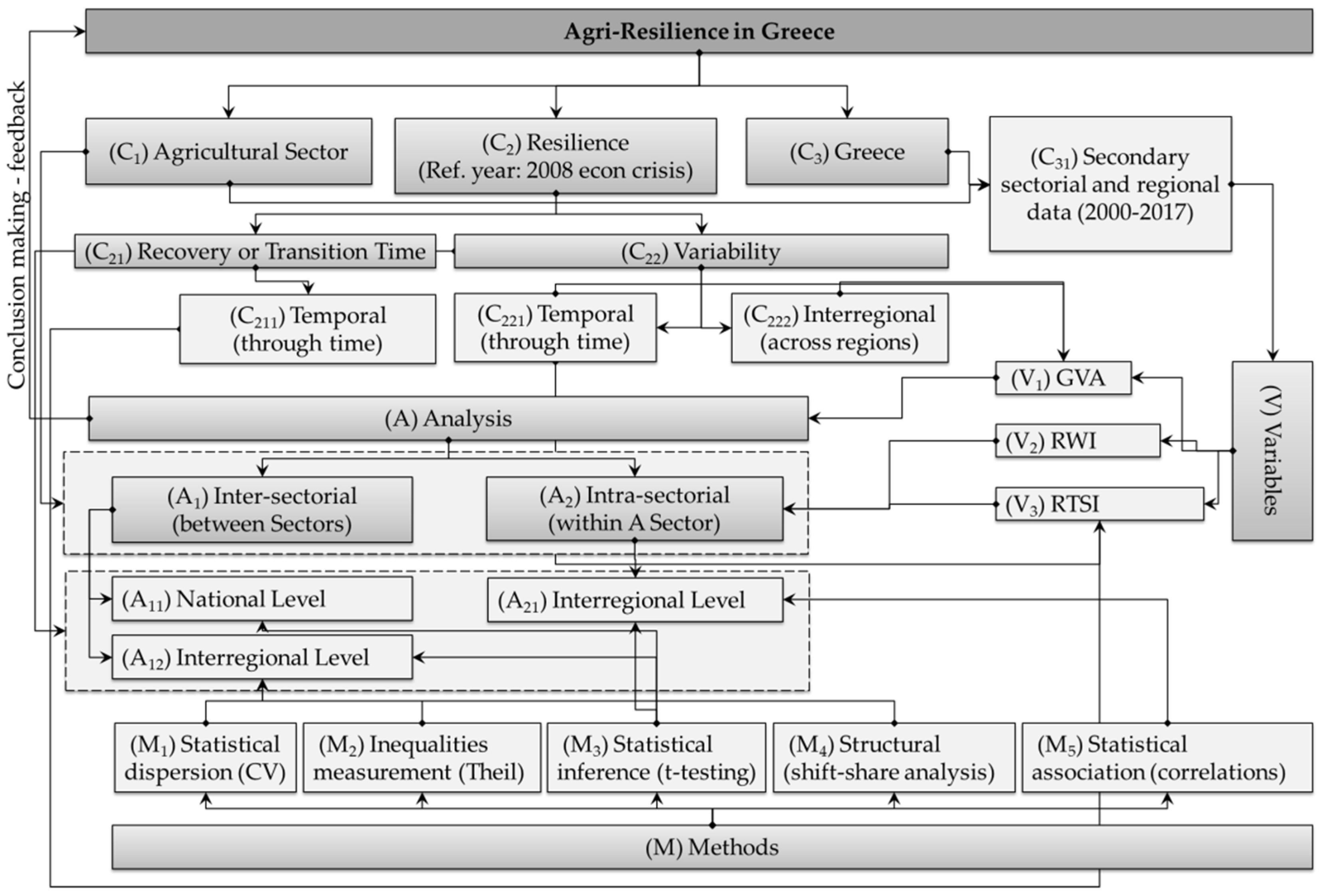
3. Methodological Framework

This paper studies the Greek agricultural sector’s resilience to the global economic crisis, according to a multilevel methodological framework shown in Figure 1. The methodological framework consists of several parts: (i) one conceptual (label: C), including the conceptual components on which the analysis is conceived; (ii) one empirical dealing with the variables’ (label: V) configuration; (iii) one including the quantitative methods (label: M) used for the analysis; and (iv) a final one concerning the analysis (label: A) applied in this study. As it can be observed, all parts of the methodological framework are interconnected, supporting diverse aspects of the multilevel analysis applied to examine the complex phenomenon of agricultural resilience in the best possible approximation. In particular, the first conceptual part (C) illustrates the diverse pillars (C₁, C₂, and C₃) composing the semantics of the subject of the study. Based on this semantic decomposition, the agricultural resilience in Greece has one dimension referring to its sectorial specialization in the agricultural sector (C₁), a second one concerning its intrinsic property (C₂) to deal with disturbances, and the third dimension concerning its geographical reference and configuration (C₃). A pair-wise consideration of these dimensions conceptually approximates, first, the industrial aspect of resilience (by combining C₁$\cup$C₂), and secondly, the regional resilience (by combining C₂$\cup$C₃), to conceive as spherical as possible the concept of resilience, as described in the introduction. The first dimension of production specialization (C₁) drives the structure of the analysis (A) to decompose into two directions: the first is comparative (A₁: between sectors analysis), examining the agricultural sector in comparison with the major other sectors of the Greek economy; and the second one is endoscopic applied within the agricultural sector (A₂). Therefore, this approach allows the study of the agricultural sector through a double perspective: its internal (A₂) and external (A₁) environment, aiming to examine the sector as spherically as possible (A₁$\cup$A₂).

The second conceptual dimension (C₂) conceives resilience as an intrinsic property. Within the context of polyphony in the literature definitions of resilience, this paper tries to conceptualize resilience both in equilibrium and evolutionary terms. This conceptualization requires defining resilience on a dual-axis: first, horizontally (C₂₁), in terms of measuring the recovering time or the time of transition to a new state of functionality (C₂₁₁) due to a shock. This approach conceives either engineering (recovering time) or ecological (transition time) resilience. In particular, measurements of recovering time within the available time interval (2008–2017) illustrate an engineering resilience performance, where longer time interprets lower resilience. If the system either does not recover or shifts to another state of functionality, the transition time is measured instead, illustrating a performance of ecological resilience. Secondly, on a vertical consideration, we define resilience in terms of capturing the variability (C₂₂) caused by the shock, approximating thus the system’s evolutionary resilience expressed as ability to adapt. In this approach, higher variability interprets less ability to resist and lower adaptability (evolutionary resilience). Provided that, for a production sector, variability may concern either its time evolution or its inequalities among its spatial (regional) units, variability also decomposes into a pair of concordant components: a temporal (C₂₂₁) and an interregional (C₂₂₂). This decomposition also drives the structure of the analysis into a double consideration; the first applies to the national (A₁₁), and the second one to the interregional level (A₂₁). Finally, the third conceptual dimension (C₃) of the methodological framework incorporates the geographical aspect, providing an empirical specialization (C₃₁) of agricultural resilience for the case of Greece.

All conceptual dimensions (C₁, C₂, and C₃) contribute to the configuration of the variables set (V) participating in the analysis. In particular, to measure the relative resilience of the agricultural sector, we use sectorial, national, and regional data of the Gross Value Added (GVA), normalized per labor unit (pLU). Among the various factors used in the literature in the study of resilience, such as GDP and aspects of productivity, employment [18], and demographic factors [25,45], the GVA variable (V₁) was chosen as a better proxy due to its better productivity configuration compared to GDP and better income configuration compared to employment, in conjunction with the data availability. In terms of data availability, GVA is the only reliable productivity variable that is available from the Greek Statistical Service [50] both in a sectorial and regional division, along with in a diachronic (time-series) setting. In terms of configuration, GVA includes more specialized production information than GDP does. In particular, while the definition of GDP also includes aspects of consumption and government spending, the GVA is free of such information [14] and therefore is preferable to GDP as a proxy of the actual regional production. Moreover, GVA has a closer configuration to income information than employment does, allowing thus constructing a framework of consistency to apply the analysis at the intra-sectorial level (A₂). The available GVA dataset refers to annual records of the period from 2000 to 2017, calculated in constant prices on the 2008-year basis. 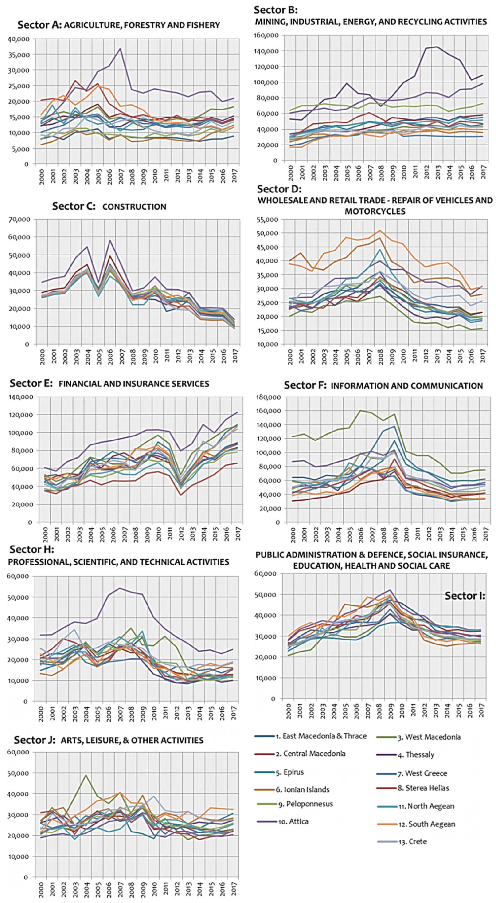Additionally, the analysis configures the Relative Workers Income (RWI) variable (V₂), which is defined by the ratio between Entrepreneurs and Employers Income and is extracted from the Hellenic Statistical Service [50] database. To facilitate comparisons, the available variables are organized into sectoral groups, according to the nine sectors shown in

Table 1. The productive sectors that are considered in the analysis.

Code	Description
Sector A	Agriculture, forestry, and fishing
Sector B	Mining and quarrying, manufacturing, electricity, gas, steam, air conditioning, and water supply, sewerage, waste management, and remediation activities
Sector C	Construction
Sector D	Wholesale and retail trade, repair of motor vehicles and motorcycles, transportation and storage, accommodation, and food service activities
Sector E	Financial and insurance activities
Sector F	Information and communication
Sector H	Professional, scientific and technical activities, and administrative and support service activities
Sector I	Public administration and defense, compulsory social security, education, human health, and social work activities
Sector J	Arts, entertainment, recreation, other service activities, activities of households as employers, undifferentiated goods and services-producing activities of households for own use, and activities of extraterritorial organizations and bodies

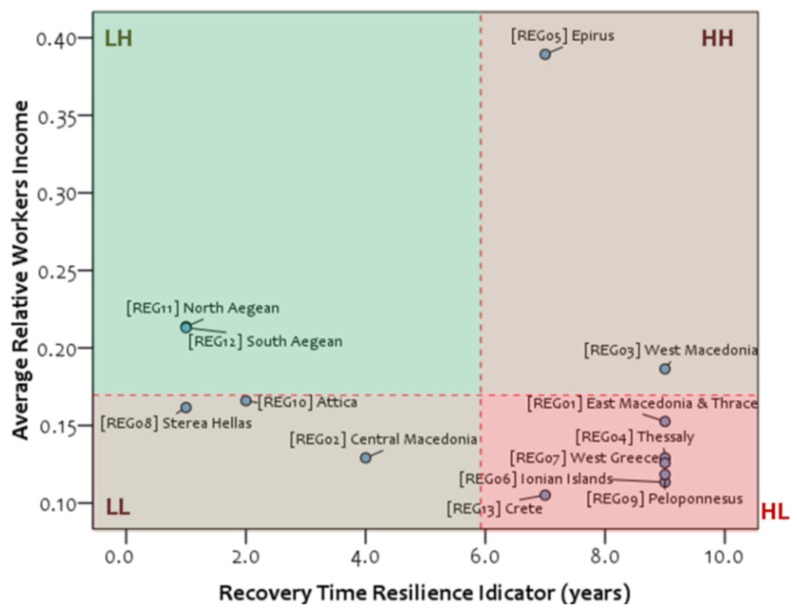
Source: [50].

. The reference sector that is used for this study is “Agriculture, forestry, and fishing” (Sector A). Finally, we configure the Recovery Time Resilience Indicator (RTSI) variable (V₃), expressing the time of recovering from the 2008 crisis and is defined by the years until to reach the least pre-crisis and on-crisis difference. Smaller values of this variable imply a faster recovery and correspond to a better resilience profile.

To study the resilience of the Greek agricultural sector (Sector A) in a comprehensive context, we apply a multilevel analysis (A) towards two sectorial (A₁, A₂) and two geographical levels; the national (A₁₁) and the interregional (A₁₂, A₂₁) level. At the national level (A₁₁), the analysis applies to temporal and sectorial data, and no regional division or segmentation is taken into account. Therefore, at this geographical level, the analysis is applicable only for the inter-sectorial consideration (A₁) and therefore computations occur to 18 annual scores (from 2000 up to 2017) of the GVA (pLU) variable (V₁). 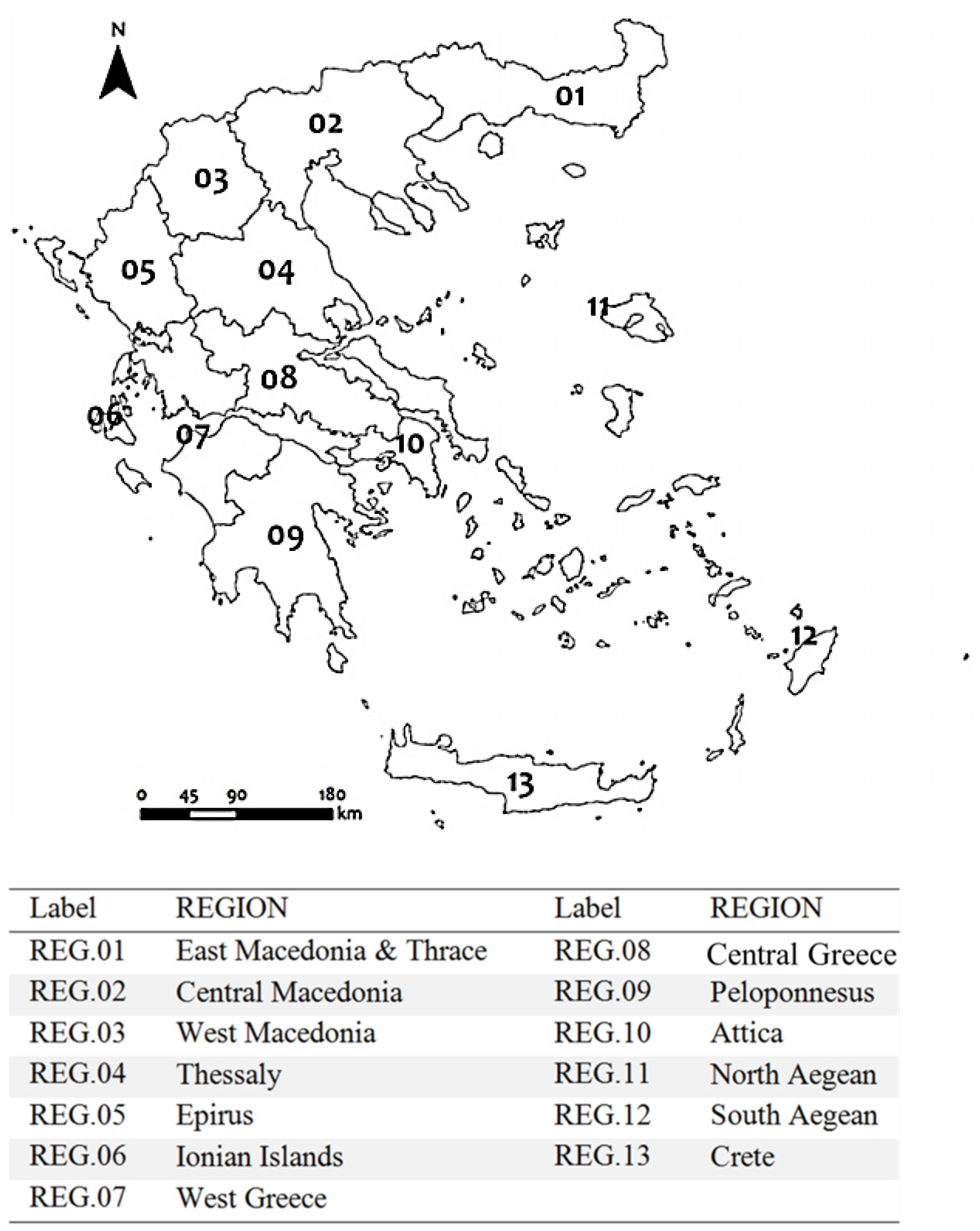On the other hand, at the interregional level (A₁₂, A₂₁), the analysis is applicable for both inter- and intra-sectorial considerations (A₁, A₂), and thus the available GVA (pLU) variable (V₁) enjoys an additional regional configuration, including annual scores of the 13 NUTS II regions of the Greek territory (Figure 2), for the period 2000–2017. Namely, at this level of analysis, the available database has a panel-data configuration, including 18 annual data tables referring to the period 2000–2017, where each panel is further organized to a regional (Figure 2) and sectorial (Table 1) grouping. For the sake of standardization, the rows in each panel correspond to regional units (NUTS II), whereas the columns correspond to the available nine major sectors of the Greek economy. The purpose of this interregional consideration (A₁₂, A₂₁) is to measure the resilience (to the extent it is expressed by data variability and inequality) through a double aspect: first, to capture the variability along the timeline and thus to measure the evolutionary aspect of resilience (C₂₂₁) within a certain regional unit; and, secondly, to capture the variability among the Greek regions and thus to measure the regional aspect (C₂₂₂) of agricultural resilience in a certain time reference.

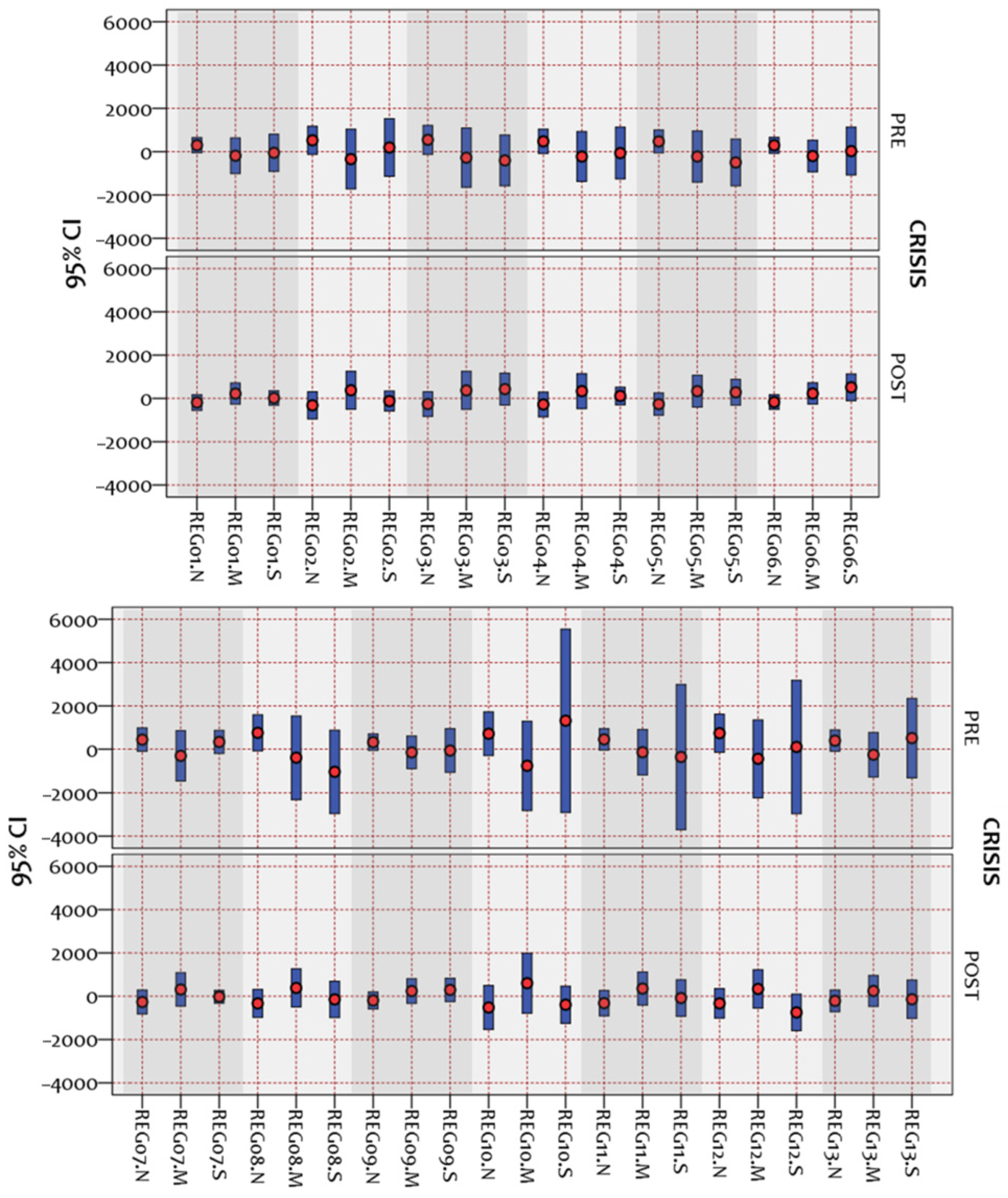
To implement the analysis, we employ a set of various methods (M), as shown in Figure 1. In particular, the inter-sectoral analysis (A₁) builds on measures of statistical dispersion (M₁) and inequalities (M₂) and employs methods of statistical inference (M₃) and structural analysis (M₄). At the national level (A₁₁), where no regional division applies to the data, the analysis builds on statistical testing (M₃) of the comparison of means between the pre- and post-crisis. Here, statistical equality between the pre-crisis (≤2008) and on-crisis (>2008) grouping implies that the system recovers from the shock and reveals an engineering aspect of resilience. On the contrary, a statistical difference indicates an ecological process (transition to another state of functionality). 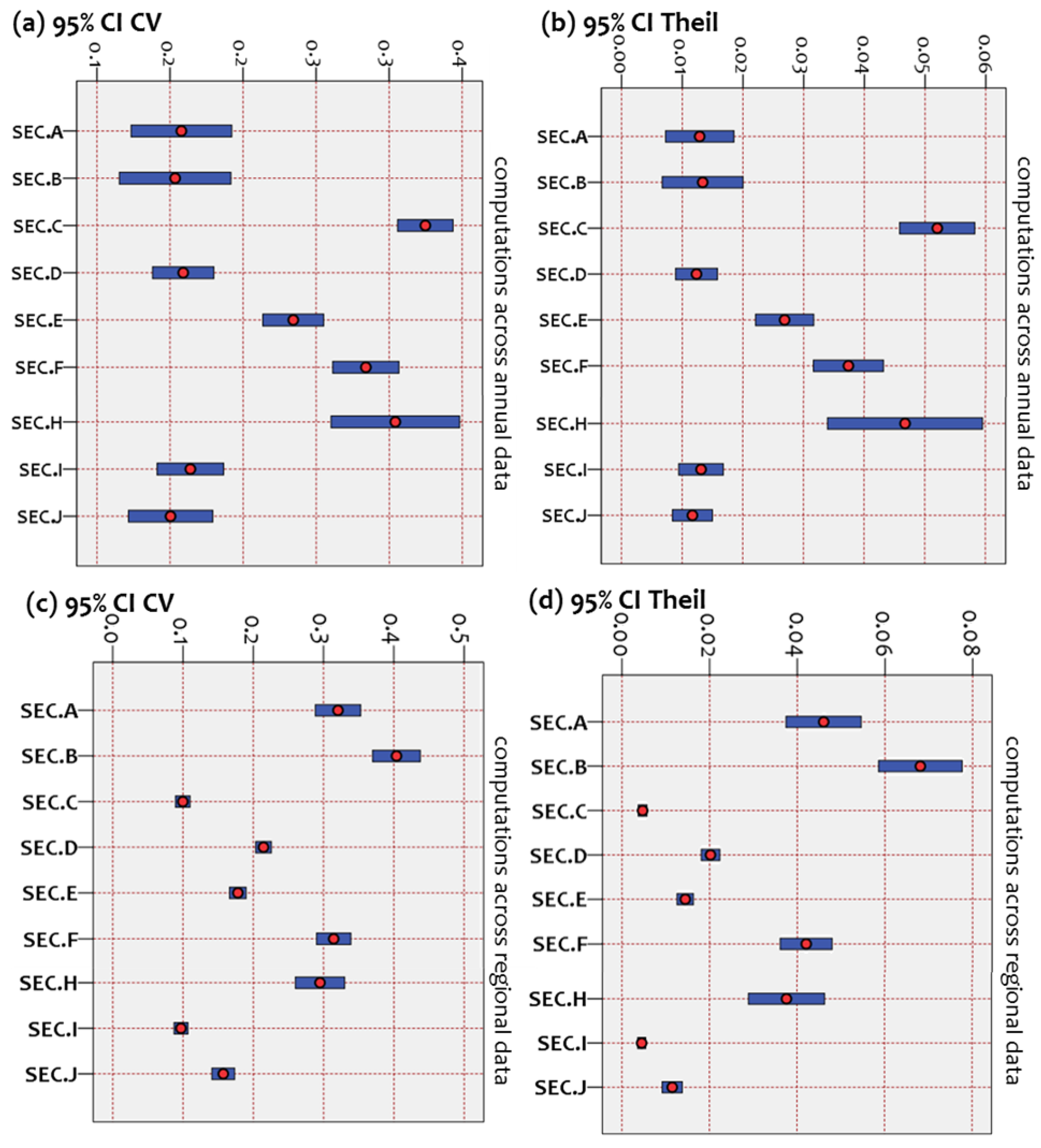At the interregional level (A₁₂), the analysis uses statistical testing (M₃), but this time it is applied to variables edited by computing the coefficient of variation—CV (M₁), the Theil index (M₂), and the shift-share analysis. Provided that the coefficient of variation (M₁) and the Theil index (M₂) capture statistical dispersion and inequalities, these measures are computed either on the temporal or regional grouping (distribution) of the dataset and therefore their results eliminate one (out of the two) groupings. Therefore, a statistical inference analysis on the data of the remaining (out of the two) distributions per industry can perform as statistical testing of either the temporal (when a measure is computed on regional data) or interregional (when a measure is computed on temporal data) magnitude and variability (inequalities) among the production sectors. According to this approach, statistical differences in the temporal mean values of the interregional inequalities indicate diverse performance between sectors in preserving interregional homogeneity along time, which can be seen as an evolutionary aspect of regional resilience. On the other hand, statistical differences in the interregional mean values of the temporal inequalities illustrate diverse performance between sectors in equivalently sharing the resilient profiles across regions, which can be seen as an aspect of regional distribution of resilience. Moreover, statistical inference on the shift-share analysis components (N, M, and S), which are computed on successive time differences for the agricultural sector, can provide further insights due to the decomposition of the temporal changes into a national (N), industrial mix (M), and local-share effect (S) component. Finally, the intra-sectorial analysis (A₂) is applicable at the interregional level (A₂₁) and builds on methods of statistical testing (M₃) and structural association (M₅). Here, statistical equality between the pre-crisis (≤2008) and on-crisis (>2008) grouping can also reveal an aspect of engineering or ecological resilience. The overall analysis aims to incorporate different aspects (C₁, C₂₁, C₂₂₁, C₂₂₂, and C₃) in the definition of resilience and thus to study this property within an integrated structural (sectorial), geographical, and evolutionary context. The particular quantitative methods [37,51,52,53,54,55,56,57,58] used to support the analysis are briefly described at the following paragraphs.

▪

Methods of statistical dispersion (M₁): The Coefficient of Variation

The coefficient of variation (CV), it is also known as the relative standard deviation, is a measure of statistical dispersion that captures the amount of homogeneity in a dataset. The coefficient is defined by the formula [56]:

$$CV=\sqrt{\mathrm{var}(x)}/\langle x\rangle ,$$

(1)

where $\sqrt{\mathrm{var}(x)}$ is the standard deviation and $\langle x\rangle$ is the mean value of the dataset. The CV measures the extent to which the observed values relatively fluctuate around the sample mean. In empirical terms, values of CV up to 10% (≤0.10) describe homogenous samples, namely, datasets with a satisfactory concentration (variability) to the mean. On the other hand, values of CV greater than 10% (>0.10) describe cases of heterogeneous samples, where a considerable dispersion from the mean can be observed [56]. The CV is by definition a unit-free (and therefore free of scale effects) coefficient because it is de-escalated by the division of the average.

▪

Methods of inequalities measurement (M₂): The Theil index

The Theil index is a measure of inequalities that belongs to the family of entropy indices, which originates from physics and generally measures the disorder of a system’s inner energy. The mathematical expression of the measure is defined as follows [53,57,58]:

$$T=\frac{1}{n}{\displaystyle \sum _{i=1}^n\frac{x_i}{\langle x\rangle }}\cdot \ln \left(\frac{x_i}{\langle x\rangle }\right),$$

(2)

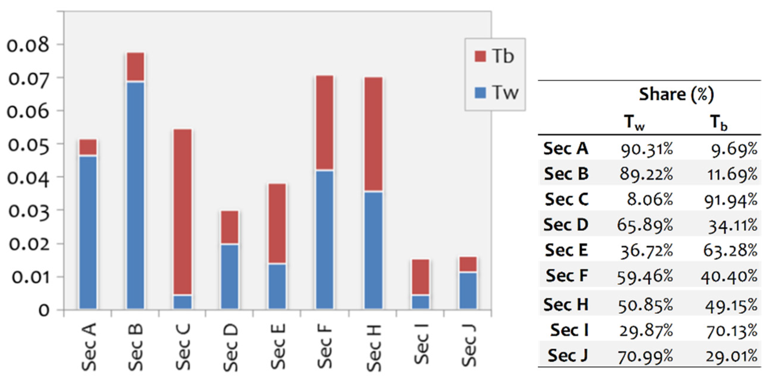
where x_i is the observed values and $\langle x\rangle$ is the mean of the dataset. The Theil index ranges between the interval 0 ≤ Τ ≤ lnn (where n is the number of cases), indicating equality in cases close to zero and perfect inequality in cases close to lnn [14]. A useful property of Theil’s index regards its ability to decompose into components when the available dataset can be divided into groups. In that case, the Theil index can decompose into a within (T_w) and a between (T_b) component, according to the relation:

$$T=\left[T_w\right]+\left[T_b\right]=\left[{\displaystyle \sum _i^{}\frac{x_i}{x}\left({\displaystyle \sum _j^{}\frac{x_{ij}}{x}}\cdot \ln (\frac{x_{ij}/x}{n_{ij}/n})\right)}\right]+\left[{\displaystyle \sum _i^{}\left(\frac{x_i}{x}\cdot \ln (\frac{x_i/x}{n_i/n})\right)}\right],$$

(3)

where

−

T is the Theil index that is computed on the total (ungrouped) dataset, as defined by relation (2);

−

T_w is the within groups component capturing the share of the Theil’s index due to the inequality within the groups;

−

T_b is the between-groups component capturing the share of Theil’s index magnitude due to the inequality between the groups;

−

$n_{ij}$ is the number of observation j of group i ($n_{ij}=1$, and $n_{ij}>1$ only if j is also a group);

−

$n_i$ is the number of observations in group i;

−

n is the number of (total) observations in all groups;

−

$x_{ij}$ is the observation belonging to the element j of group i; and

−

$x={\displaystyle \sum _i^{}{\displaystyle \sum _j^{}{x}_{ij}}}=n\mu$ is the sum of all observations, across all groups.

▪

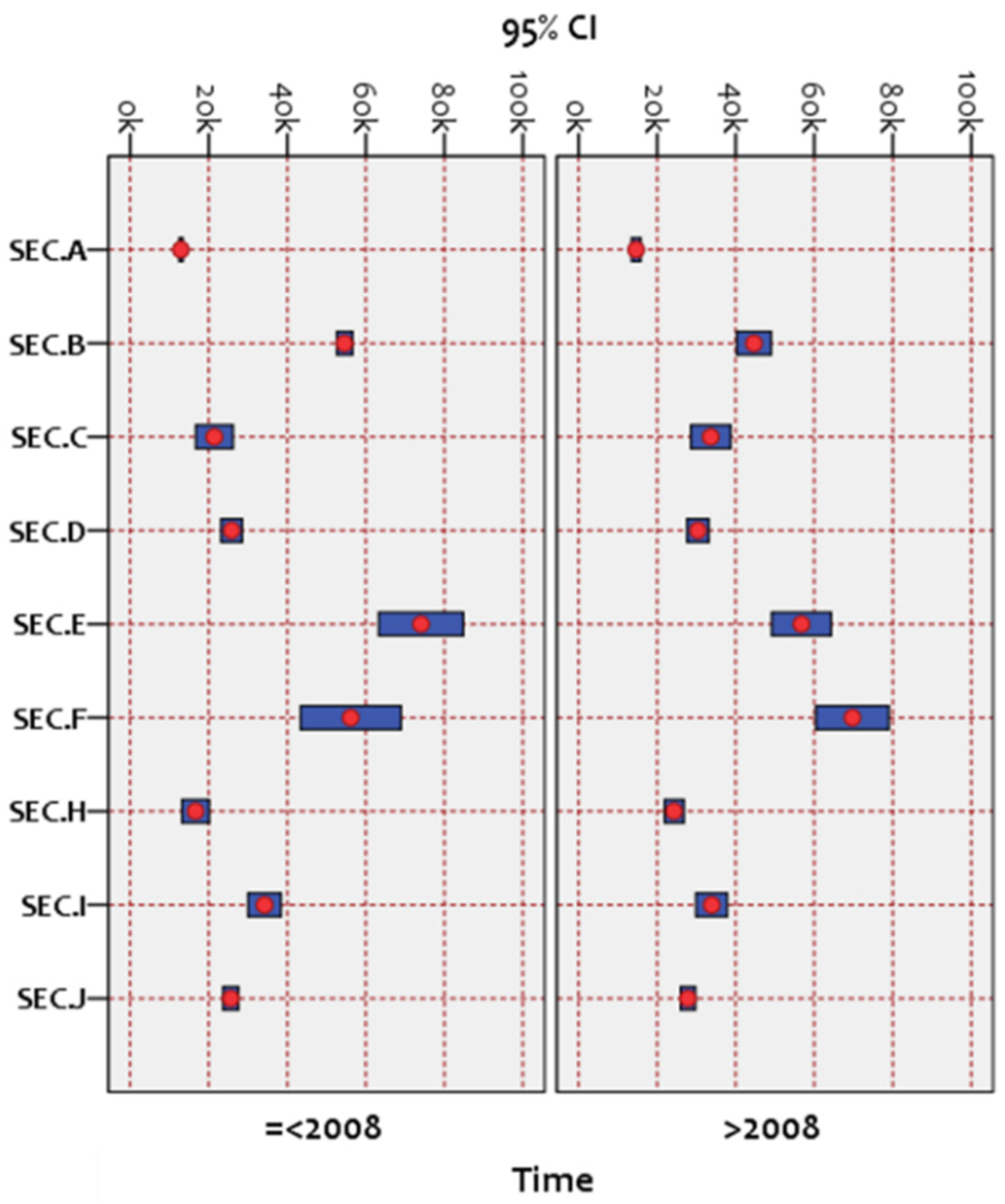
Methods of statistical testing (M₃): The independent-samples t-test

Except for the previous measures and indicators of variability and inequalities, the analysis builds on statistical and empirical methods to extract information from the available data. Therefore, the independent-samples t-test is used to compare the means μ_α and μ_β (in 0.05 significance level) between two discrete groups defined from the same variable X by using either an arithmetic (i.e., cutting point) or categorical grouping criterion. 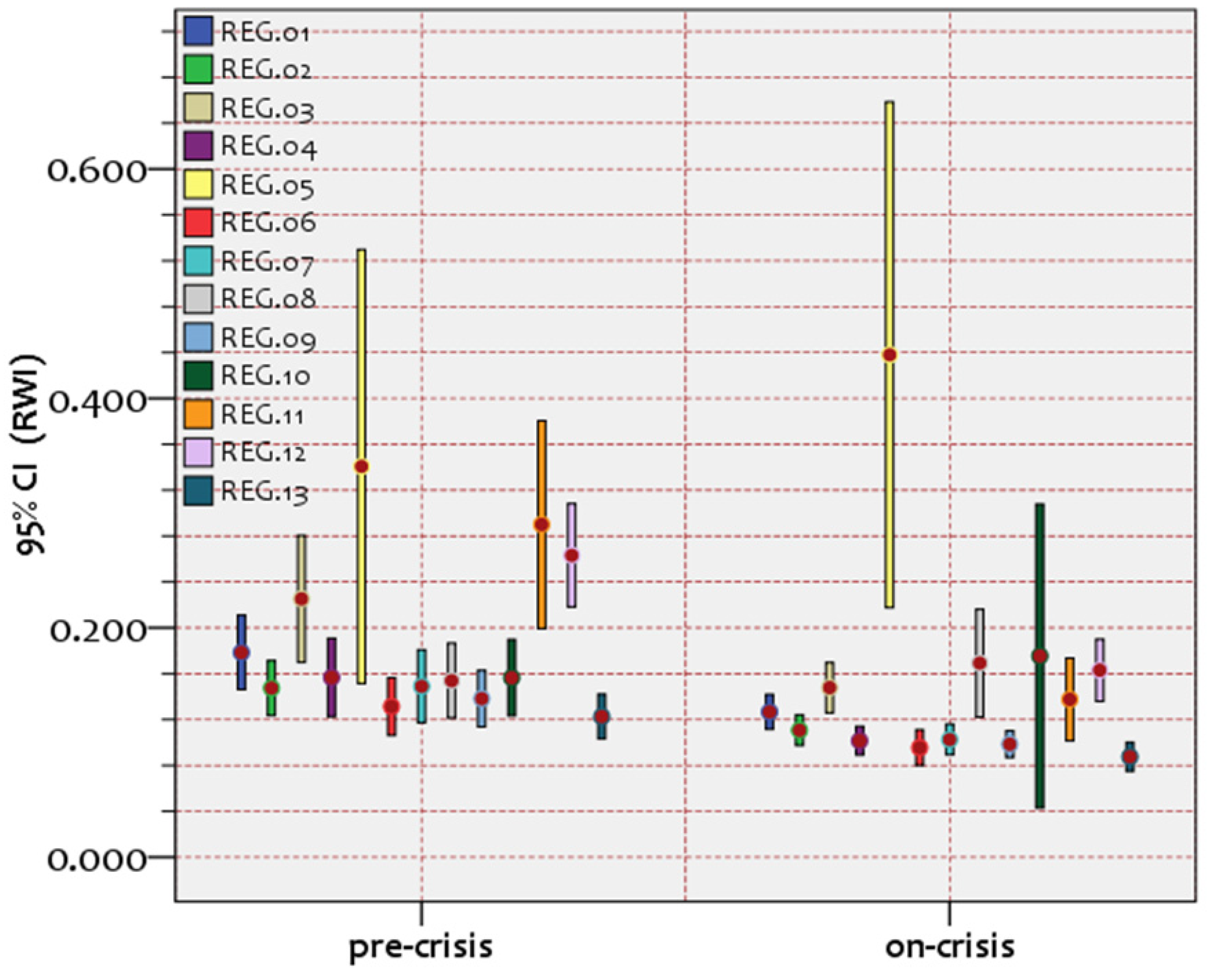This approach utilizes Levene’s test for the examination of the equality of variances between the groups and produces separate results for unpooled and pooled variances that are valid depending on their significance [55,56]. A visualization of this test can be achieved by using error bars of 95% confidence intervals (CIs) for the means. In general, 95% CIs are computed by default in the tests, and the missing values are excluded pair-wisely, namely, the algorithm keeps from test to test the max possible degrees of freedom to perform the analysis [56].

▪

Methods of structural analysis (M₄): The shift-share analysis (M₄)

The shift-share analysis builds on the concept of decomposition, as the Theil index does, which further allows the attainment of structural information due to a grouping [14,37]. However, instead of decomposing a quantity, a shift-share method is based on the decomposition of differences expressing the change in an attribute, for a certain time. Within this context, a shift-share analysis is a summative expression defined by the relation:

$$\begin{array}{l}\Delta X_{ir}(t_1,t_o)=\left(X_{ir}(t_1)-X_{ir}(t_o)\right)\equiv R_{ir}(t_1,t_o)=\\ =N_{ir}(t_1,t_o)+M_{ir}(t_1,t_o)+S_{ir}(t_1,t_o),\end{array}$$

(4)

where R_ir is the change in a quantity (attribute) X referring to sector i and region r between time t = t_o and t = t₁, component N_ir is the so-called national growth effect that is defined by the relation $N_{ir}=X_{iro}\left[\frac{X_{nt}}{X_{no}}\right]-X_{iro}$ and expresses the share of change in X that is attributed to the total growth of the national economy, component M_ir is the so-called industrial mix effect that is defined by the relation $M_{ir}=X_{iro}\left[\frac{X_{int}}{X_{ino}}-\frac{X_{nt}}{X_{no}}\right]$ and expresses the share of change in X that is attributed to the certain sectoral structure of the economy, and component S_ir is the so-called local-share effect that is defined by the relation $S_{ir}=X_{irt}-X_{iro}\frac{X_{int}}{X_{ino}}$ and expresses the share of change in X that is attributed to the regional influences of the economy. The term M_ir + S_ir is also known as the shift component expressing any share of change that is attributed to not the total growth of the national economy [14,37]. The shift-share analysis is expected to provide added value to the analysis of this paper because it will interpret the variability of changes in the GVA in terms of a (sectorial) spatio-economic grouping of the available data.

▪

Methods of statistical association (M₅): The correlation analysis

Finally, a correlation analysis based on Pearson’s bivariate coefficient of correlation is applied to detect a linear association between the available variables (V₁, V₂, and V₃). The coefficient of correlation is defined by the ratio [55,56]:

$$r_{XY}=\left(\mathrm{cov}(X,Y)\right)/\left(\sqrt{\mathrm{var}(X)}\cdot \sqrt{\mathrm{var}(Y)}\right)$$

(5)

where cov(X,Y) is the covariance of variables X,Y, and $\sqrt{\mathrm{var}(\cdot )}$ is the sample standard deviations. Pearson’s coefficient of correlation ranges within the interval (−1,1) and detects linear relations when it reaches asymptotically $\left|r_{XY}\right|\to 1$. A visualization of correlation between variables is achieved by using scatterplots [55,56].

4. Results

4.1. Inter-Sectorial Analysis (A₁) at the National Level (A₁₁)

At the first step of the analysis, we examine the GVA (pLU) of the available Greek sectors (Table 1) at the national levels. The results of the analysis are shown in the line diagram of Figure 3, which illustrates the sectorial GVA (pLU) time-series of Greece for the period 2000–2017, and in the error-bars of Figure 4, which illustrate a t-test for the equality of means within each sector prior (≤2008) and on (>2008) the economic crisis. As can be observed in Figure 3, the time evolution of the GVA (pLU) per sector in Greece shapes a rather fluctuated picture. At this macroscopic level, some productive sectors seem to perform better than others. In particular, Sector B (Energy resources) can be considered as the sector with the best engineering resilience, since the pre-crisis (≤2008) maximum of its time-series is recovered just one year after the economic crisis (in 2010). After 2010, the GVA (pLU) of this sector kept growing, indicating an ecological process of resilience driving the system to a higher state of functionality. Moreover, Sector E (Financial and insurance activities) can be considered as a sector with engineering and ecological resilience because not only does it succeed in recovering to the pre-crisis (≤2008) maximum (engineering process) but it also moved to a state of higher functionality (ecological process). However, all the other sectors did not succeed to recover to their pre-crisis functionality (lack of engineering resilience) and they consequently moved to a new lower state (illustrating a performance of “negative” ecological resilience). This is also the case of the agricultural sector (Sector A), which did not succeed to recover to its pre-crisis functionality and it, therefore, moved to a new state of lower functionality. Even worse, the agricultural sector counts the minimum numerical values of GVA (pLU) in the period 2000–2017 compared to the other sectors. Similarly, Sector H (Professional, scientific, and technical activities) shows a minimum GVA (pLU) performance after 2013, and Sector C (Construction) has a minimum in the year 2017.

To further evaluate the effect of the economic crisis on the resilience of sectorial productivity, we apply independent sample t-tests for the equality of means between the pre- (≤2008) and on-crisis (>2008) groups per sector, as is shown in the error-bars of Figure 4. In terms of average, sectors A (Agriculture, forestry, and fishing), C (Construction), D (Trade, Transportation, and Tourism Services), and H (Professional, Scientific, Technical, Administrative, and Support Services) cannot be considered resilient in engineering terms, because they did not (statistically) recover to their pre-crisis average GVA (pLU) level (functionality). At a glance, this result for the tourism sector (D) may appear contradictory with the findings of [25,49], who observed that Greek regions specialized in tourism appeared more resistant to the 2008 economic crisis. However, by considering the variability as denoted by level error bars’ length, we can observe that the variability of sector D is considerably small, illustrating an aspect of stability through time. These low levels of variability interpret an evolutionary resilience profile for sector D, to the extent that low variability implies a good resistance in changes through time and thus high levels of adaptability. Within this context, the performance of sector D in Figure 4 is in line with the findings of [25,49], who appear to highlight the sector’s evolutionary resilience, but are also complementary because they provide insights into the lack of engineering resilience of the tourism sector. Based on this double consideration that the error bars of Figure 4 can provide, sectors A, C, D, and H may lack engineering resilience but are equipped with evolutionary resilience. Among these cases, sector A has the shortest error bars’ length, illustrating a good evolutionary performance.

On the other hand, sectors E (Financial and insurance activities), F (Information and communication), I (Public administration and social care), and J (Arts, entertainment, recreation, other service activities) can be considered (in terms of average) as resilient in engineering terms because their pre-crisis and on-crisis GVA (pLU) average are statistically equal. However, the error bars of sectors E and F are of great variability, not allowing a safe interpretation of their evolutionary performance without further consideration. According to Figure 3, sector E shapes a high-fluctuated on-crisis picture, described by a sudden drop in 2012 and a fast sequential recovery, implying a good performance of adaptability. On the other hand, F shows a successive decline after 2008 lying at similar levels of magnitude of the oldest pre-crisis levels. Except for the detected good engineering performance, this picture describes a deficient performance of adaptability and thus evolutionary resilience. Compared to all cases, Sector B (Energy resources) can be overall considered as the most resilient because: (i) its on-crisis average GVA (pLU) outperforms the concordant pre-crisis score, illustrating both an engineering process (recovery to the previous state of functionality) and an ecological process (shift to a state of higher functionality); and (ii) is described by low levels of variability, related to a good evolutionary performance. This observation illustrates the inelastic demand for energy of national economies [59,60], showing an increasing trend regardless of the significant external shock caused by the 2008 economic crisis. Overall, this (two-step) inter-sectorial analysis provides insights into considering, first, Sector B (Energy resources) as an overall most resilient sector, secondly, sector E (Financial and insurance activities), F (Information and communication) as a case of considerable engineering and ecological resilience, and, finally, sectors A, D, H, and J as cases of evolutionary resilience.

4.2. Inter-Sectorial Analysis (A₁) at the Interregional Level (A₁₂)

In the second part, the analysis applies to variables with a regional (NUTS II) configuration (Figure 2). At first, the sectorial GVA (pLU) time-series of Greece are examined at their regional grouping, as shown in the line diagrams of Figure 5.

These diagrams appear rather fluctuated both along the timeline and across the regional cases, making their interpretation rather complex and necessitating further analysis. This observation highlights the methodological requirement of this paper to measure sectorial resilience through a double temporal (within a certain regional unit and throughout a period) and geographical (within a certain time reference and across different regions) aspect. Despite their high level of complexity, these diagrams (Figure 5) can provide prime insights into a considerable interregional homogeneity (as denoted by small variability captured across regions) of sectors C, I, and secondarily E and J (see nomenclature in Table 1). In terms of temporal variability (approximating an aspect of evolutionary resilience), a picture of small fluctuations along the time-axis can be observed for sectors B, J, and A.

To evaluate whether the average performance differs between the period before (≤2008) and after (>2008) the economic crisis, for each sector (i = 1, …, 9) and region (j = 1, …, 13), we apply an Independent Samples t-test for the comparison of means. The results of the analysis are shown in

Table 2. Significant variables ^1,2 of the Independent Samples t-test applied for the mean GVA (pLU) differences Δμ = μ_≥2008–μ_<2008, per sector (i = SEC.A:SEC.J) and region (j = 1:13) ³.

Region	SECTOR A	SECTOR B	SECTOR C	SECTOR D	SECTOR E	SECTOR F	SECTOR H	SECTOR I	SECTOR J
1		SEC.B.1	SEC.C.1	SEC.D.1	SEC.E.1	SEC.F.1	SEC.H.1		SEC.J.1
2		SEC.B.2	SEC.C.2	SEC.D.2			SEC.H.2
3		SEC.B.3	SEC.C.3	SEC.D.3	SEC.E.3	SEC.F.3			SEC.J.3
4		SEC.B.4	SEC.C.4	SEC.D.4	SEC.E.4	SEC.F.4	SEC.H.4
5			SEC.C.5	SEC.D.5	SEC.E.5		SEC.H.5
6		SEC.B.6	SEC.C.6	SEC.D.6	SEC.E.6	SEC.F.6
7			SEC.C.7	SEC.D.7			SEC.H.7
8	SEC.A.8		SEC.C.8		SEC.E.8		SEC.H.8		SEC.J.8
9			SEC.C.9	SEC.D.9	SEC.E.9		SEC.H.9
10		SEC.B.10	SEC.C.10		SEC.E.10	SEC.F.10	SEC.H.10
11		SEC.B.11	SEC.C.11	SEC.D.11	SEC.E.11	SEC.F.11	SEC.H.11
12	SEC.A.12	SEC.B.12	SEC.C.12		SEC.E.12		SEC.H.12
13		SEC.B.13	SEC.C.13		SEC.E.13		SEC.H.13

¹ At 0.05 level of significance; ² Full numerical results are shown in the Appendix A (Table A1); ³ Negative differences are shown in red and positive in green color.

, where we can observe that: (i) Sector A counts two regions (j = 8, and 12) with statistically different means between the pre-crisis and on-crisis period; (ii) Sector B counts nine (j = 1–4, 6, and 10–13) regions; (iii) Sector C counts all thirteen (j = 1–12) regions; (iv) Sector D counts nine (j = 1–7, and 9–10) regions; (v) Sector E counts eleven (j = 1, 3–6, and 8–13) regions; (vi) Sector F counts six (j = 1, 3–4, 6, 10, and 11) regions; (vii) Sector H counts eleven (j = 1–2, 4–6, and 7–13); (viii) Sector I does not count any case; and (ix) Sector J counts three (j = 1, 3, and 8) regions. According to the conceptual framework of the study: (i) a significant positive statistical difference in the GVA (pLU) means Δμ = μ_≥2008 − μ_<2008, between the pre-crisis (≤2008) and on-crisis (>2008) period, can reveal aspects of engineering (ability to recover from a shock) and positive ecological (transition to a higher level of functionality) resilience of a system; (ii) a significant negative statistical difference can be seen as an aspect of negative ecological resilience (i.e., implying that the system shifts to a state of lower functionality due to the disturbance); and (iii) an insignificant statistical difference can be seen as an aspect of engineering resilience (the systems recover to their previous state of functionality). Within this context, the results of the Independent Samples t-tests imply: (i) that the most engineering and ecological resilient sectors are E, with 11/13 positively significant (positive ecological resilience) and 2/13 insignificant (engineering resilience) differences, and B, with 9/13 positively significant (positive ecological resilience) and 4/13 insignificant (engineering resilience) differences; and (ii) that the most engineering resilient sectors are I, with 13/13 insignificant differences, A, with 11/13 insignificant differences, and J, with 10/13 insignificant differences.

For a more in-depth analysis, we compute the coefficient of variation (CV) and the Theil index, to evaluate the level of variability and inequalities of the GVA (pLU) per sector. In particular, we perform the calculations per sector on a double basis. On the one hand, we compute these measures across annual data (of GVA (pLU), which produce one measure per region (CV_r, T_r, r = 1, 2, …, 13), for a sector. On the other hand, we compute these measures across the regional data, which produce one measure per year (CV_t, T_t, t = 2000, 2001, …, 2017), for a sector. This two-dimensional approach allows t-tests for the equality of the means of the CV and the Theil index among the sectorial variables to be applied, and thus the homogeneity level in each sector to be evaluated, both along the regional (geographical) and temporal (time, across annual data) dimensions. The results of this analysis are shown in Figure 6, where it can first be observed from the first two figures (Figure 6a,b) that sectors C, E, F, and H have on average statistically greater annual inequalities (as denoted by the numerical values in the horizontal axes) among the Greek regions than the other sectors. To the extent that high inequalities (or variability) can be seen as an aspect of low evolutionary resilience for a system, this result interprets that sectors A, B, D, I, and J are the most evolutionary resilient ones. In terms of interregional inequalities (Figure 6c,d), sectors A, B, F, and H have on average statistically greater interregional inequalities (on an annual basis) than the other sectors. This result concordantly interprets that sectors C, D, E, I, and J can be considered as the most homogeneous in terms of their regional configuration through time (which can be loosely seen as an aspect of regional resilience).

Next, Figure 7 shows the results of the Theil index decomposition into within (T_w) and between (T_b) groups components. This analysis configures all available GVA (pLU) scores into annual groups (g₁ = 2000, g₂ = 2001, …, g₁₈ = 2017) and then calculates the within and between groups variability according to Theil’s decomposition process. As it can be observed, for sectors C, E, and H, the share in the Theil index’s configuration is mainly due to the inequalities between, rather than within, the groups. These inequalities are related to the variability caused by the time evolution of the GVA (pLU) rather than the variability caused by the interregional differentiation. On the other hand, for sectors A, B, D, F, I, and J, the share in the Theil index’s configuration is mainly due to the inequalities within, rather than between, the groups, implying that the major data variability is configured by the interregional rather than the temporal inequalities. This part of the analysis reveals that sectors A and B are the most resilient through time but very unevenly distributed in their geographical configuration, whereas Sector C is the least resilient through time but the most evenly distributed in their geographical configuration, as is also evident by the line diagrams in Figure 5.

At the final part of the analysis, the available GVA (pLU) scores are analyzed by using a shift-share analysis, aiming to interpret the variability of the GVA (pLU) changes in terms of the spatio-economic structure of the available data. By computing the shift-share components N_ir(t,t + 1), M_ir(t,t + 1), and S_ir(t,t + 1), for all available regions r = 1, …, 13, sectors i = 1, …, 9, and time steps t = 2000, …, 2016, we apply independent sample t-tests for the equality of means, to evaluate the pre- (≤2008) and on-crisis (>2008) performance of the regions, for the N, M, and S components of the agricultural sector (A). The results of the analysis are shown in Figure 8, and are arranged into triplet groups (N, M, and S)_r per region r = 1, …, 13. As it can be observed, for all the available cases, no statistically significant difference between the pre- and on-crisis performance of the regional shift-share components appears, which implies that it cannot be statistically concluded that the economic crisis significantly affected the magnitude of the national, industrial mix, and differential effects in the share of changes in the GVA (pLU). This observation implies that the national, sectorial, and interregional configuration in the GVA (pLU) structure of Greece was insignificantly affected by the 2008 economic crisis. However, the variability (as expressed by the CIs length) that is observed in the on-crisis period (>2008) appears considerably lower, implying a trend of that period’s temporal inequalities (and thus of the national, sectorial, and interregional configuration in the GVA (pLU) structure) to converge. Overall, the analysis applied at the interregional level provided insights into the temporal and sectorial dimension of the regional resilience of the Greek sectors’ productivity, as is expressed by the GVA (pLU) per labor variable. This composite approach allows capturing different aspects of regional resilience incorporating different aspects of its geographical configuration and thus evaluating the geographical and temporal dynamics of this property.

4.3. Intra-Sectorial Analysis (A₂) at the Interregional Level (A₂₁)

In this part analysis, we examine the Relative Workers Income (RWI) in the agricultural sector, which is defined by the ratio of the workers’ to the employers’ income (both referring to Sector A). The RWI expresses the proportion of the workers’ to the employers’ income (essentially, it describes how well-paid the workers in each region are, relative to their employers), and thus it can be seen as an indicator of the level of “quality” of the workers’ contribution to the agricultural configuration of the regional economy. The available RWI data concern annual records of the period 2000–2017, per region, and are measured in euros (EUR). The analysis consists of three parts: in the first, we evaluate the relevance between RWI and their corresponding GVA variables of the Greek regions for the agricultural sector, by applying a Pearson’s bivariate correlation analysis [55,56]; in the second part, we correlate the temporal RWI average with the Recovery Time Resilience Indicator (RTSI); and in the third part, we examine the effect of crisis to the regional RWI configuration.

The results of the correlation analysis between the RSI and GVA variables are shown in

Table 3. Pairwise correlations between diachronic variables (2000–2017) of the Relative Workers Income and Gross Value Added (both for the agricultural sector), configured at the national level and for the 13 Greek regions.

Region (NUTS II)	Variable X	Variable Y	Pearson Correlation	Sig. (2-Tailed)	N
Greece	RWI.GR	GVA.GR	0.744 **	0.000	18
East Macedonia & Thrace	RWI.01	GVA.01	0.502 *	0.034
Central Macedonia	RWI.02	GVA.02	0.625 **	0.006
West Macedonia	RWI.03	GVA.03	−0.109	0.667
Thessaly	RWI.04	GVA.04	0.114	0.652
Epirus	RWI.05	GVA.05	−0.061	0.809
Ionian Islands	RWI.06	GVA.06	−0.013	0.960
West Greece	RWI.07	GVA.07	0.680 **	0.002
Central Greece	RWI.08	GVA.08	−0.250	0.318
Peloponnesus	RWI.09	GVA.09	0.085	0.738
Attica	RWI.10	GVA.10	0.057	0.824
North Aegean	RWI.11	GVA.11	−0.164	0.515
South Aegean	RWI.12	GVA.12	0.842 **	0.000
Crete	RWI.13	GVA.13	0.711 **	0.001

** Correlation is significant at the 0.01 level (2-tailed); *. Correlation is significant at the 0.05 level (2-tailed); Cases shown in bold font imply significant correlations.

. As it can be observed, at the national level (first row), the RWI is highly correlated (>0.7) with the GVA variable, implying that the patterns of variability between these two variables are relevant. This relevance describes that in more profitable years, where the GVA in agriculture is higher, workers are likely more to also enjoy higher shares of income (relatively to their employers) than other years. This correlation can illustrate the effect of workers’ income on national productivity, but this relation is not linear. Moreover, significant correlations between RWI and GVA are observed for the regions of East Macedonia and Thrace, Central Macedonia, West Greece, South Aegean, and Crete, illustrating a considerable relevance between workers income and regional productivity. Especially for the insular region of South Aegean, the correlation is higher than the national score. Provided that tourism is a basic sector in this region [14], this result provides insights into the cooperativeness between the agricultural and tourism sectors and implies that tourism specialization can promote agricultural production into higher worker incomes, complying with relevant findings [25,49] stating the better resilience profiles of regions that are more specialized to tourism.

Next, Figure 9 shows the correlation between the temporal average RWI and the RTSI (defined as the number of years after 2008 until to reach the least pre-crisis and on-crisis difference). To the extent that RTSI can be seen as an engineering resilience indicator, this correlation analysis can provide insights based on the “production quality” of the agricultural sector (RWI). By considering the means per variable, we can divide the correlation panel into quadrants, pair-wisely expressing the profile (LL = low RWI, low RTSI, LH = low RWI, high RTSI, etc.) of each region. As it can be observed, the regions belonging to the best performance quadrant (LH) are the North Aegean (REG.11) and South Aegean (REG.12), which have a small recovery time and a high proportion of the workers’ income. Within the context that these regions are the two components of the geographical department of the Aegean Sea, which is the most developed region in tourism [14], their LH performance provides more evidence into the cooperativeness between the agricultural and tourism sectors that was previously observed. On the other hand, the regions belonging to the lowest performance quadrant (HL) are East Macedonia and Thrace (REG.01), Thessaly (REG.04), Ionian Islands (REG.06), West Greece (REG.07), Peloponnesus (REG.09), and Crete (REG.13), which have high recovery time and low proportion of the workers’ income. Finally, the regions belonging to the moderate performance quadrants (LL, and HH) are the regions of central mainland Greece. Overall, this analysis shows that the relationship between RWI and RTSI (as an aspect of engineering resilience) is interestingly geographically driven.

Finally, we apply Independent Samples t-tests for the comparison of means of the RWI variable between the pre- (≤2008) and on-crisis (>2008) groups. The results are shown in Figure 10, where it can be observed that only regions 5 (Epirus) and 8 (Central Greece) did not significantly change their averages due to the crisis. To the extent that insignificant statistical differences (about the economic crisis) can be seen as aspects of engineering resilience and significant differences as an aspect of ecological (positive or negative) resilience, the results of these t-tests imply that the engineering resilience of the agricultural sector is rather low across the regions since only 2/13 do not significantly change their mean RWI due to the crisis. Moreover, this result complies with the findings of Figure 6c,d describing that, although Sector A appears resilient in evolutionary terms, it is very unevenly distributed in its geographical configuration.

5. Discussion

Based on the previous literature review and analysis, economic resilience is undoubtedly a composite concept inheriting a high level of complexity describing spatial–economic systems. One dimension of such complexity regards the economic configuration of a system, driving into the industrial conceptualization of resilience. Another dimension regards the geographical partition of the system, driving into a regional specialization (or reference) of resilience. Another dimension concerns the performance of the economic or regional system over time, thus conceptualizing resilience either as an engineering, ecological, or evolutionary process. Within this complex framework, to approximate economic resilience as spherically as possible, this paper focused on the resilience of the agriculture in Greece (which, for decades, been a developing sector of the country) to the 2008 economic crisis and applied a multilevel analysis at different industrial (inter-sectorial and intra-sectorial) and geographical (national, interregional) levels, and by using various measures and methods to capture diverse conceptualizations of resilience. In particular, the engineering aspect of resilience, which describes the potential of the system to recover to its previous state of functionality, was measured in terms of recovering time to the pre-crisis average and in terms of statistically examining pre-crisis (≤2008) and on-crisis (>2008) differences. The ecological aspect of resilience, which describes the process driving a system to a new state of (higher or lower) functionality, was conceived in terms of statistical differences between the pre-crisis (μ_≤2008) and on-crisis (μ_>2008) averages. Positive differences (Δμ > 0) indicate that the system moves to a higher state of functionality, illustrating an engineering mechanism. On the other hand, negative differences (Δμ < 0) indicate that the system moves to a state of lower functionality, illustrating an ecological process. Finally, the evolutionary aspect of resilience, which describes the adaptability of a system to continuously changing conditions, was conceived in terms of variability observed through time, where low cases are seen as aspects of good evolutionary resilience.

This multilevel approach applies in an attempt to approximate as spherically as possible and to highlight the importance of an integrated conceptualization of economic resilience. However, some limitations are also inevitably applicable in this study, mainly concerning modeling restrictions. A first limitation regards the data origin, which is inevitably determinative to the representativeness of the system described. The authors of [29] noted that the attribute on which resilience is examined is determinative for the outcome of the study, and demonstrated the differences that may occur between the use of GDP and employment in the empirical framework of European regions. Although we provide documentation for using the GVA as a better proxy in this study, the using in the intra-sectorial analysis (A₂₁) of additional variables related to employment, which is considered by many researchers as a reliable attribute for measuring resilience [18], is an attempt to further overcome (or counterbalance) this limitation. Another limitation regards the acceptance of normality in the sample distributions of the data for the hypotheses testing methods [56] that apply in this study. Although this limitation is conditionally for these methods, the configuration of the multilevel framework consisting of various methodological approaches employing a synthetic outcome is an attempt to counterbalance this and other similar restrictions. Within this context, the analysis was applied toward three directions, one inter-sectorial (A₁) at the national level (A₁₁), one inter-sectorial (A₁) at the interregional level (A₁₂), and one intra-sectorial (A₂) at the interregional level (A₂₁). The results of the overall multilevel analysis are summarized in

Table 4. Summary table with the resilience profiles extracted from the inter-sectorial and intra-sectorial analysis.

	Inter-Sectorial Analysis at the National Level (A11)					Inter-Sectorial Analysis at the InterreGional Level (A12)				Intra-Sectorial Analysis at the Interregional Level (A21)
	Ranking		Engineering profile	Ecological profile	Evolutionary profile	Engineering profile 1	Ecological profile	Evolutionary profile 2	Regional resilience 2	Engineering profile	Ecological profile	Evolutionary profile
	Pre-crisis level	On-crisis level
Sector A	9	9				84.6%	15.4%	9.69%
Sector B	3	3				30.8%	69.2%	11.69%
Sector C	7	4					100.0%		8.06%
Sector D	5	6				30.8%	69.2%	34.11%	65.89%
Sector E	1	2				15.4%	84.6%		36.72%
Sector F	2	1				53.8%	46.2%
Sector H	8	8				15.4%	84.6%
Sector I	4	5				100.0%		70.13%	29.87%
Sector J	6	7				23.1%	76.9%	29.01%	70.99%
								LEGEND
									Positive
									negative
								1.	Grading based on regional proportion
								2.	Grading based on inequalities measurement

and are organized by the conceptual aspects (engineering, ecological, and evolutionary) of resilience and the industrial structure of Greece taken into consideration.

First, the inter-sectorial analysis (A₁) at the national level (A₁₁) showed that the agricultural sector (A) lacks engineering resilience to the 2008 economic crisis, leading to a state of lower functionality (as the majority of sectors in Greece). This undesirable performance worsens, even taking into account that the sector ranks last in the GVA (pLU) levels, compared to the other sectors. However, one positive aspect about the performance of the agricultural sector in Greece concerns its low levels of temporal variability, describing a profile of evolutionary resilience. This result interprets agriculture in Greece as a production sector of notable adaptability through time, addressing, thus, avenues for investments and development under low risk. Within an inter-sectorial context, the analysis showed first that sector B overall enjoys (in all three aspects: engineering, ecological, and evolutionary) good performance of resilience, probably highlighting the inelastic national demand for energy. Secondly, it showed that sector E enjoys a considerably good performance of resilience (in two aspects: engineering and ecological), which is probably related to the potential of financial and insurance activities to grow in uncertain times. A similar, but more specialized, picture is also shaped by the inter-sectoral analysis (A₁) at the interregional level (A₁₂), which first verifies the agricultural sector’s ecological and evolutionary resilience profile observed at the national scale. However, this analysis shows, in more detail, that 84.6% of the Greek regional configuration of the agricultural sector is described by engineering resilience and that the national lack of engineering resilience (as observed in the previous analysis) in the agricultural sector is a matter of a 15.4% of regions with a dominant performance. In inter-sectorial terms, this analysis also verifies the leading resilience performance of sector B, and provides further insights into considering sectors D, E, I, and J as sectors of considerable regional resilience. Finally, the intra-sectorial analysis (A₂) at the interregional level (A₂₁) highlighted (in line with the previous findings): (i) the negative ecological profile of the agricultural sector, as a result, more of regional inequalities than temporal variability; (ii) a promising evolutionary profile of resilience for the sector; (iii) the cooperativeness between the agricultural and tourism sectors as a promising developmental avenue; and (iv) revealed geographical trends in the configuration of the engineering performance of the Greek regions in agriculture.

According to the previous analysis, the agricultural sector in Greece appears adaptable over time but considerably poor in absolute terms and insufficient to recover to the past levels of higher prosperity. This overall picture is probably a result of the geomorphological, infrastructure, and functional handicaps of the country, some major issues are (but are not constrained to): (i) the considerably low share of arable and (ii) irrigated per capita land, (iii) the constraint variability of cultivations, and (iv) the low level of technological integration in the agricultural productivity [12,14]. Towards an attempt to upgrade the lagging resilience profile (mainly concerning the engineering and ecological aspects) of the agricultural sector in Greece, agricultural policies should apply into a double-axis: (i) first, towards improving the share of agriculture in the national economy; and (ii) secondly, into the reduction in the regional inequalities in agricultural productivity and income. Towards the first axis, good practices that can be extracted from the literature, may—among others—concern: (i) merging of arable land to provide benefits of cost reduction and economies of scale [14]; (ii) motivating the employment of labor of high-level qualification and a relatively youthful population [18]; (iii) a further restructuring of crops and the successful marketing of products [46]; (iv) supporting microeconomic economy (family and neighborhood) [25] and local industries [22], to enhance household economic resilience [41]; and (v) promoting land-use diversification as an instrument of risk splintering [13,41]. Next, policies towards the second axis may—among others—regard: (i) investments for enlarging irrigated cultivations [12,14]; (ii) upgrading technological support of cultivations [14]; (iii) bottom-up oriented (place-based instead of across space) regional policies [26] with emphasis on small-scale localized activities [25], local agricultural industries, and local industrial strategies [22]; and (iv) increase in agricultural productivity of less developed regions to improve their competitive advantage [12].

6. Conclusions

This paper is built on a multilevel quantitative framework of statistical and decomposition techniques to examine the level at which the agricultural (compared to eight other sectors) sector of the Greek economy was resilient through time. To this end, the economic resilience was conceptualized within a three-dimensional framework composed of a temporal, geographical, and sectorial (operational) dimension and was quantified within the context of the engineering, ecological, evolutionary, industrial, and regional aspects of resilience that are available in the literature, with regard to the 2008 economic crisis. In this multidimensional context, economic resilience was measured in terms of recovering time to pre-crisis maxima (providing insights into engineering processes), of statistical testing differences between the pre-crisis and on-crisis averages (providing insights into engineering and ecological processes), and calculating the variability (providing insights into evolutionary processes), on data referring to the Gross Value Added variable (pLU) that were organized per sector, region, and annual basis. The analysis showed that the agricultural sector (A) in Greece lacks engineering resilience because it did not recover to its maximum pre-crisis performance and moved to a state of lower functionality, expressing a negative ecological resilience profile. Moreover, in terms of the numerical scale, Sector A was described by the least numerical GVA (pLU) values, verifying the relevant literature about the poor dynamics of agriculture in Greece. Moreover, the analysis revealed that the geographical configuration of Sector A across regions is very unevenly distributed, highlighting that a major deficiency is the spatial asymmetry of its developmental dynamics. However, a positive aspect of the performance of the Greek agricultural sector regards its low levels of temporal variability, describing a profile of evolutionary resilience, which interprets agriculture in Greece as a production sector of notable adaptability. Finally, the analysis illustrated the cooperativeness between the agricultural and tourism sectors, providing insights into considering this relationship as a promising developmental avenue, along with avenues of regional development building on encouraging investments and developing economies of agglomeration and scale, for the agricultural sector. The multilevel consideration of this paper introduces (but is not restricted to) avenues of further research; one towards a further quantitative or methodological integration of the diverse ecological, engineering, evolutionary aspects of resilience; another towards including additional sectors for examining their industrial resilience; one towards studying whether sectorial structure may correlate with the diverse ecological, engineering, evolutionary aspects of resilience; and another towards studying whether geographical properties may correlate with these diverse aspects of resilience. Overall, the analysis provided insights both into the methodological conceptualization and management of regional resilience and the case study of the structural analysis of the regional rural economy of Greece.

References

1. Ahnstrom, J.; Hockert, J.; Bergea, H.L.; Francis, C.A.; Skelton, P.; Hallgren, L. Farmers and nature conservation: What is known about attitudes, context factors and actions affecting conservation? Renew. Agric. Food Syst. 2009, 24, 38–47. [Google Scholar] [CrossRef] [Green Version]
2. Herman, A. Enchanting resilience: Relations of care and people–place connections in agriculture. J. Rural Stud. 2015, 42, 102–111. [Google Scholar] [CrossRef]
3. Lemonakis, C.; Vassakis, K.; Zopounidis, C.; Voulgaris, F. Efficiency, competitiveness and exports of agricultural firms in the on-crisis era: Evidence from Greece. Int. J. Soc. Syst. Sci. 2016, 8, 14–35. [Google Scholar] [CrossRef]
4. Niavis, S.; Vlontzos, G. Seeking for Convergence in the Agricultural Sector Performance under the Changes of Uruguay Round and 1992 CAP Reform. Sustainability 2019, 11, 4006. [Google Scholar] [CrossRef] [Green Version]
5. Irz, X.; Lin, L.; Thirtle, C.; Wiggins, S. Agricultural productivity growth and poverty alleviation. Dev. Policy Rev. 2001, 19, 449–466. [Google Scholar] [CrossRef]
6. European Commission. A Framework for Indicators for the Economic and Social Dimensions of Sustainable Agriculture and Rural Development; European Commission, Agriculture Directorate-General: Brussels, Belgium, 2001; Available online: https://ec.europa.eu/agriculture/publi/reports/sustain/index_en.pdf (accessed on 11 October 2002).
7. Lichtfouse, E.; Navarrete, M.; Debaeke, P.; Souchère, V.; Alberola, C.; Menassieu, J. Agronomy for sustainable agriculture: A review. Sustain. Agric. 2009, 13, 1–7. [Google Scholar]
8. Loizou, E.; Karelakis, C.; Galanopoulos, K.; Mattas, K. The role of agriculture as a development tool for a regional economy. Agric. Syst. 2019, 173, 482–490. [Google Scholar] [CrossRef]
9. Volkov, A.; Zickiene, A.; Morkunas, M.; Balezentis, T.; Ribasauskiene, E.; Streimikiene, D. A Multi-Criteria Approach for Assessing the Economic Resilience of Agriculture: The Case of Lithuania. Sustainability 2021, 13, 2370. [Google Scholar] [CrossRef]
10. Papadopoulos, A.G.; Fratsea, L.M.; Karanikolas, P.; Zografakis, S. Reassembling the Rural: Socio-Economic Dynamics, Inequalities and Resilience in Crisis-Stricken Rural Greece. Sociol. Rural. 2019, 59, 474–493. [Google Scholar] [CrossRef]
11. Polyzos, S.; Tsiotas, D. Measuring structural changes of the Greek economy during the period of economic crisis. Manag. Res. Pract. 2020, 12, 5–24. [Google Scholar]
12. Polyzos, S.; Arabatzis, G. Labor productivity of the agricultural sector in Greece: Determinant factors and interregional differences analysis. Univ. Thessal. Dep. Plan. Reg. Dev. Discuss. Pap. Ser. 2005, 11, 209–226. [Google Scholar]
13. Andreoni, V.; Duriavig, M. Economic Resilience and Land use: The Cocoa Crisis in the Rio Cachoeira Catchment, Brazil. Environ. Policy Gov. 2013, 23, 118–129. [Google Scholar] [CrossRef]
14. Polyzos, S. Regional Development, 2nd ed.; Kritiki: Athens, Greece, 2019; ISBN 9789602187302. (In Greek) [Google Scholar]
15. Simmie, J.; Martin, R. The economic resilience of regions: Towards an evolutionary approach. Camb. J. Reg. Econ. Soc. 2010, 3, 27–43. [Google Scholar] [CrossRef] [Green Version]
16. Lee, N. Grim down South? The Determinants of Unemployment Increases in British Cities in the 2008–2009 Recession. Reg. Stud. 2014, 48, 1761–1778. [Google Scholar] [CrossRef]
17. Martin, R.; Sunley, P. On the notion of regional economic resilience: Conceptualization and explanation. J. Econ. Geogr. 2014, 15, 1–42. [Google Scholar] [CrossRef] [Green Version]
18. Kitsos, A.; Bishop, P. Economic resilience in Great Britain: The crisis impact and its determining factors for local authority districts. Ann. Reg. Sci. 2018, 60, 329–347. [Google Scholar] [CrossRef] [Green Version]
19. Buheji, M. Reviewing How ‘Creating Resilient Economies’ can Help Developing Countries in Uncertain Times. Am. J. Econ. 2019, 9, 259–263. [Google Scholar]
20. Bristow, G.I.; Healy, A.; Norris, L.; Wink, R.; Kafkalas, G.; Kakderi, C.; Espenberg, K.; Varblane, U.; Sepp, V.; Sagan, I.; et al. ECR2. Economic Crisis: Regional Economic Resilience; Project Report; ESPON: Brussels, Belgium, 2014. [Google Scholar]
21. Capello, R.; Caragliu, A.; Fratesi, U. Spatial heterogeneity in the costs of the economic crisis in Europe: Are cities sources of regional resilience? J. Econ. Geogr. 2015, 15, 951–972. [Google Scholar] [CrossRef]
22. Kitsos, A.; Carrascal-Incera, A.; Ortega-Argiles, R. The Role of Embeddedness on Regional Economic Resilience: Evidence from the UK. Sustainability 2019, 11, 3800. [Google Scholar] [CrossRef] [Green Version]
23. Schwarz, A.-M.; Bene, C.; Bennett, G.; Boso, D.; Hilly, Z.; Paul, C.; Posala, R.; Sibiti, S.; Andrew, N. Vulnerability and resilience of remote rural communities to shocks and global changes: Empirical analysis from Solomon Islands. Glob. Environ. Chang. 2011, 21, 1128–1140. [Google Scholar] [CrossRef]
24. Brakman, S.; Garretsen, H.; Van Marrewijk, C. The Crisis and Regional Resilience in Europe: On the Importance of Urbanization and Specialization; Working Paper; CESifo Group: Munich, Germany, 2014. [Google Scholar]
25. Psycharis, Y.; Kallioras, D.; Pantazis, P. Economic crisis and regional resilience: Detecting the ‘geographical footprint’ of economic crisis in Greece. Reg. Sci. Policy Pract. 2014, 6, 121–141. [Google Scholar] [CrossRef]
26. Palaskas, T.; Psycharis, Y.; Rovolis, A.; Stoforos, C. The asymmetrical impact of the economic crisis on unemployment and welfare in Greek urban economies. J. Econ. Geogr. 2015, 15, 973–1007. [Google Scholar] [CrossRef]
27. Tsiapa, M.; Batsiolas, I. Firm resilience in regions of Eastern Europe during the period 2007–2011. Post Communist Econ. 2019, 31, 19–35. [Google Scholar] [CrossRef]
28. Martin, R.; Sunley, P.; Gardiner, B.; Tyler, P. How Regions React to Recessions: Resilience and the Role of Economic Structure. Reg. Stud. 2016, 50, 561–585. [Google Scholar] [CrossRef] [Green Version]
29. Sensier, M.; Bristow, G.; Healy, A. Measuring Regional Economic Resilience across Europe: Operationalizing a complex concept. Spat. Econ. Anal. 2016, 11, 128–151. [Google Scholar] [CrossRef]
30. Xiao, J.; Boschma, R.; Andersson, M. Resilience in the European Union: The effect of the 2008 crisis on the ability of regions in Europe to develop new industrial specializations. Ind. Corp. Chang. 2017, 27, 15–47. [Google Scholar] [CrossRef] [Green Version]
31. Martin, R.; Gardiner, B. The resilience of cities to economic shocks: A tale of four recessions (and the challenge of Brexit). Pap. Reg. Sci. 2019, 98, 1–32. [Google Scholar] [CrossRef]
32. Karrholm, M.; Nylund, K.; de la Fuente, P.P. Spatial resilience and urban planning: Addressing the interdependence of urban retail areas. Cities 2014, 36, 121–130. [Google Scholar] [CrossRef]
33. Morkunas, M.; Volkov, A.; Pazienza, P. How resistant is the agricultural sector? Economic resilience exploited. Econ. Sociol. 2018, 11, 321–332. [Google Scholar] [CrossRef]
34. Michel-Villarreal, R.; Vilalta-Perdomo, E.; Hingley, M.; Canavari, M. Evaluating economic resilience for sustainable agri-food systems: The case of Mexico. Strateg. Chang. 2019, 28, 279–288. [Google Scholar] [CrossRef]
35. Pnevmatikos, T.; Polyzos, S.; Tsiotas, D. Assessing the structural changes in the Greek economy for the period prior to economic crisis. Reg. Sci. Inq. 2019, 11, 69–82. [Google Scholar]
36. Suryahadi, A.; Suryadarma, D.; Sumarto, S. The effects of location and sectoral components of economic growth on poverty: Evidence from Indonesia. J. Dev. Econ. 2009, 89, 109–117. [Google Scholar] [CrossRef]
37. Polyzos, S.; Tsiotas, D.; Sdrolias, L. Greek regional productivity at the period of the economic crisis: Obtaining information by using Shift–Share analysis. MIBES Trans. Int. J. 2013, 7, 92–109. [Google Scholar]
38. Polyzos, S.; Tsiotas, D.; Niavis, S. Analyzing the Location Decisions of Agro-Industrial Investments in Greece. Int. J. Agric. Environ. Inf. Syst. IJAEIS 2015, 6, 77–100. [Google Scholar] [CrossRef]
39. Giannakis, E.; Bruggeman, A. Economic crisis and regional resilience: Evidence from Greece. Pap. Reg. Sci. 2017, 96, 451–476. [Google Scholar] [CrossRef]
40. Dijkstra, L.; Garcilazo, E.; McCann, P. The effects of the global financial crisis on European regions and cities. J. Econ. Geogr. 2015, 15, 935–949. [Google Scholar] [CrossRef]
41. Chonabayashi, S.; Jithitikulchai, T.; Qu, Y. Does agricultural diversification build economic resilience to drought and flood? Evidence from poor households in Zambia. Afr. J. Agric. Resour. Econ. 2020, 15, 65–80. [Google Scholar] [CrossRef]
42. Quendler, E.; Morkunas, M. The Economic Resilience of the Austrian Agriculture since the EU Accession. J. Risk Financ. Manag. 2020, 13, 236. [Google Scholar] [CrossRef]
43. Christopherson, S.; Michie, J.; Tyler, P. Regional resilience: Theoretical and empirical perspectives. Camb. J. Reg. Econ. Soc. 2010, 3, 3–10. [Google Scholar] [CrossRef]
44. Cheng, L.; Zhang, J. Is tourism development a catalyst of economic recovery following natural disaster? An analysis of economic resilience and spatial variability. Curr. Issues Tour. 2020, 23, 2602–2623. [Google Scholar] [CrossRef]
45. Giannakis, E.; Bruggeman, A. Regional disparities in economic resilience in the European Union across the urban–rural divide. Reg. Stud. 2020, 54, 1200–1213. [Google Scholar] [CrossRef]
46. Papaelias, T.; Panagou, V.; Hyz, A. The developments and trends of the agricultural sector in Greece. Zesz. Nauk. Szkoły Głównej Gospod. Wiej. Warszawie Probl. Rol. Swiat. 2014, 14, 108–115. [Google Scholar]
47. Christofakis, M.; Gkouzos, A. Regional specialisation and efficiency of the agricultural sector in Greece: The relationship with regional funding allocation. Reg. Sect. Econ. Stud. 2013, 13, 119–130. [Google Scholar]
48. Kalantzi, O.; Tsiotas, D.; Polyzos, S. The contribution of tourism in national economies: Evidence of Greece. Eur. J. Bus. Soc. Sci. EJBSS 2016, 5, 41–64. [Google Scholar]
49. Petrakos, G.; Psycharis, Y. The spatial aspects of economic crisis in Greece. Camb. J. Reg. Econ. Soc. 2016, 9, 137–152. [Google Scholar] [CrossRef]
50. Hellenic Statistical Service—ELSTAT. Gross Added Value per Sector. 2021. Available online: https://www.statistics.gr/el/statistics/-/publication/SEL12/ (accessed on 5 September 2021).
51. Berzeg, K. The empirical content of shift-share analysis. J. Reg. Sci. 1978, 18, 3. [Google Scholar] [CrossRef]
52. Knudsen, D.C. Shift-share analysis: Further examination of models for the description of economic change. Socio Econ. Plan. Sci. 2000, 34, 177–198. [Google Scholar] [CrossRef]
53. Clements, K. Henri Theil, 1924–2000. Int. J. Forecast. 2001, 17, 141–142. [Google Scholar] [CrossRef]
54. Dinc, M. Regional and Local Economic Analysis Tools; The World Bank: Washington, DC, USA, 2002. [Google Scholar]
55. Norusis, M. IBM SPSS Statistics 19.0 Guide To Data Analysis; Prentice Hall: Hoboken, NJ, USA, 2011. [Google Scholar]
56. Walpole, R.E.; Myers, R.H.; Myers, S.L.; Ye, K. Probability & Statistics for Engineers & Scientists, 9th ed.; Prentice Hall Publications: New York, NY, USA, 2012. [Google Scholar]
57. Tsiotas, D.; Polyzos, S. The contribution of ANN’s simple perceptron pattern to inequalities measurement in Regional Science. Oper. Res. Int. J. 2013, 13, 289–301. [Google Scholar] [CrossRef]
58. Tsiotas, D.; Sdrolias, L.; Aspridis, G.; Skodova-Parmova, D.; Dvorakova-Liskova, Z. Size distribution analysis in the study of urban systems: Evidence from Greece. Int. J. Comput. Econ. Econom. 2021, 11, 12–36. [Google Scholar] [CrossRef]
59. Menegaki, A.N. Growth and renewable energy in Europe: A random effect model with evidence for neutrality hypothesis. Energy Econ. 2011, 33, 257–263. [Google Scholar] [CrossRef]
60. Menegaki, A.N. On energy consumption and GDP studies; A meta-analysis of the last two decades. Renew. Sustain. Energy Rev. 2014, 29, 31–36. [Google Scholar] [CrossRef]
Figure 1. Semantic diagram of the methodological framework of the study.
Agriculture 12 00174 g001
Figure 2. The Greek NUTS II regions (source: [50]).
Agriculture 12 00174 g002
Figure 3. Line diagrams with the sectorial GVA per labor unit (pLU) time-series of Greece, shown at the national level, for the period 2000–2017. GVA prices are measured in EUR/LU (constant prices on 2008 basis).
Agriculture 12 00174 g003
Figure 4. Error bars illustrating t-tests for the equality of means of GVA (pLU) for the pre- (≤2008) and on-crisis (>2008) grouping, for each sector. GVA prices are measured in EUR/LU (constant prices on 2008 basis).
Agriculture 12 00174 g004
Figure 5. Line diagrams showing the sectoral time-series of the Gross Value Added (GVA) (pLU) for 13 Greek regions (NUTS II), during the period 2000–2017. GVA prices are measured in EUR/LU (constant prices on 2008 basis).
Agriculture 12 00174 g005
Figure 6. Error bars of 95% CI for the mean value of: (a) the coefficient of variation (CV) and (b) the Theil index, per sector, where the measures’ computations applied across annual data of GVA (pLU). Error bars of 95% CI for the mean value of (c) the CV and (d) the Theil index, per sector, where the measures’ computations applied across regional data of GVA (pLU). GVA prices measured in EUR/LU (constant prices on 2008 basis).
Agriculture 12 00174 g006
Figure 7. Stacked bars showing the contribution of each component (Tw,Tb) to the configuration of the Theil index, per sector (annual grouping), where the measures’ computations were applied to GVA (pLU) data. GVA prices are measured in EUR/LU (constant prices on 2008 basis).
Agriculture 12 00174 g007
Figure 8. Error bars of 95% CIs of the pre-and on-crisis mean values of the shift-share analysis components (R, N, M, and S), for the 13 (NUTS II) Greek regions (the measures’ computations applied across annual GVA (pLU). GVA prices are measured in EUR/LU (constant prices on 2008 basis).
Agriculture 12 00174 g008
Figure 9. Correlation scatter plot, between the diachronic average Relative Workers Income (RWI) and the Recovery Time Resilience Indicator (RTSI) variable.
Agriculture 12 00174 g009
Figure 10. Error bars of 95% CIs of the pre-and on-crisis mean values of the Relative Workers Income (RWI) variable, computed for the 13 (NUTS II) Greek regions (computations across annual data).
Agriculture 12 00174 g010