Article

Labour Commutation in the Agricultural Sector—An Analysis of Agricultural Workers in Chile

by
Claudio Mancilla
1,*,
Luz María Ferrada
1,
Sergio Soza-Amigo
2,* and
Adriano Rovira
3
1
Department of Administrative and Economic Sciences, Universidad de Los Lagos, Osorno 5290000, Chile
2
Instituto de Gestión e Industria, Universidad Austral de Chile, Puerto Montt 5480000, Chile
3
Facultad de Ciencias Económicas y Administrativas, Instituto de Turismo, Universidad Austral de Chile, Valdivia 5090000, Chile
*
Authors to whom correspondence should be addressed.
Agriculture 2022, 12(12), 2110; https://doi.org/10.3390/agriculture12122110
Submission received: 11 October 2022 / Revised: 6 December 2022 / Accepted: 7 December 2022 / Published: 9 December 2022

Abstract

:
Agricultural activity is a key strategic sector for countries, particularly for food production. One way to strengthen the sector is through the use of technology. However, while integrating new technologies, challenges have emerged in the sector with regard to incorporating workers. Thus, one way to resolve this workforce shortfall could be through labour commutation, which consists of people living in one territory but working in another. Therefore, this study aims to analyse the likelihood of agricultural workers becoming worker commuters. Chile is used as a case study, drawing on the Chilean National Employment Survey of 2018 to analyse differences among the five largest regions in the country: Great North, Small North, Central Zone, South, and Chilean Patagonia. Each zone possesses different characteristics, and a propensity score matching process was carried out within the data. The results indicate that agricultural workers with a higher education level, full-time jobs, working in the formal sector, and younger workers are more likely to commute. Different impacts of variables were found across the zones. However, most of the variables have similar impact on the likelihood to commute in different areas. Thus, from a labour perspective, public policies can create general incentives to attract a new workforce to strengthen the agricultural sector.

1. Introduction

Agricultural activities have seen a significant drop in their contribution to countries’ GDP worldwide [1], and their current competitiveness depends not only on their ability to incorporate new technologies but also on meeting workforce demand. However, agricultural activities face challenges regarding the quality and quantity of workers available. Despite this, the agricultural sector remains critically important in developing countries because of the employment it provides and its contribution to food security [2].
The origin of labour shortages is multi-causal and not exclusive to the sector. At the same time, spatial mobility of labour exists in primary sectors, with some of the people working in these sectors residing in a different geographical area from where they work. Living in one territory but working in another is known as commutation. It appears to be particularly worthy of study in the agricultural sector because it could be a mechanism for attracting labour. However, the percentage of workers who commute in the agricultural sector is lower than in other economic sectors.
Several studies address labour commuting in Chile, which is the case study used in this research. However, works with a focus on agricultural activities are scarce; those that exist focus on other economic sectors or examine agriculture from a more global perspective.
This paper, thus, seeks to answer the following question: What are the characteristics of agricultural workers who commute and what variables influence greater commutation? Therefore, the study’s primary objective is to analyse an agricultural worker’s probability of commuting.
We adopted two quantitative strategies to achieve this objective: applying a logit model to the data and carrying out a data-matching process. More specifically, the probabilities that workers in the agricultural sector could commute were calculated on the basis of socio-demographic characteristics. Additionally, differences in results among five zones of the country were evaluated (Great North, Small North, Central, South, and Chilean Patagonia). These areas include different climates, different population densities, and different productive specialisations.
This paper is structured in five sections, including this Introduction; it is followed by Section 2, which contains the Literature Review, examining commutation and antecedents to detail the Chilean context and agricultural activity; Section 3, Materials and Methods, contains a description of the database, variables, and quantitative methods used in this research; Section 4 presents the Results; and Section 5 presents the Discussion and Conclusions.

2. Antecedents and Theorical Framework

2.1. Agricultural Employment: The Case of Chile

According to Alston and Pardey [3], agricultural output per capita in the long-term is rising but remains comparatively less dynamic than other sectors of the economy. This is a worldwide phenomenon and translates into a loss of relative importance (share) of the sector in the total GDP of countries [4]. This aligns with the fact that farmers in some countries have indicated that they have had difficulties in finding workers [5].
These trends are similar in several countries, and in Latin America, where agriculture is still very important, the sector faces challenges for the future, such as further improving productivity and climate change. In Chile, the case studied in this paper, the agricultural sector is a competitive industry with a leading position in the continent in producing several goods; it is also a dynamic activity requiring increasingly specialised labour skills. Despite the above, there is a great deal of heterogeneity within the country, with both a high-tech agricultural sector and a low-tech sector, with workers exhibiting a low level of schooling [6,7].
In the case of Chile, between 1996 and 2020, the agricultural sector’s share of the total GDP dropped—although not as dramatically as the fall in agricultural employment. This can be seen in Figure 1, where it is possible to observe the participation in GDP; in global terms, its relative importance has decreased or maintained in recent years. Agricultural employment between these years fell to less than half, even in 2020, when the COVID-19 pandemic began. In other words, this also reflects an increase in productivity.
The incorporation of technology into the sector explains the fall in the share of agricultural employment and productivity improvement. Some reports have indicated that for Chile, the supply of agricultural employment could fall by 5.8% or even 12%, depending on the type of work or contract. The same reports indicated that eventually the labour shortage would disappear thanks to the deployment of technology in the sector but that it would require workers with higher levels of qualifications [8,9]. However, for several years, the sector has been exhibiting a labour supply shortage, regardless of the level of training supposedly required.
However, over several years at the international level, it has been postulated that some of the reasons for the decrease in the supply of agricultural employment are the ageing population and people’s higher levels of training [10].

2.2. Labour Commutation

Labour commutation is understood as workers living in a territory other than the one in which they work. In other words, these workers do not migrate or establish themselves permanently in the place of work.
Spatial labour commuting is a mechanism that improves the efficiency of the labour market by providing workers to the labour markets where they are needed. In the Chilean context, some researchers have studied commutation and the incentives available in mining activities and areas (North Zone of the country). Although there is migration of workers to these areas, it is increasingly common for people to move for work without changing their place of residence, i.e., they are commuters. Thus, there has been an increase in long-distance commuting from the 1990s to the first decade of this century [11].
The literature explains this change in behaviour through greater access to better road infrastructure, new means of transport, and lower transport costs [12]. In turn, it is argued that commuting is associated with labour productivity and the wage expectations of commuters [13]. Thus, it has been shown that commuting for labour reasons increases the distance as wages increase, i.e., the regions that receive more commuters are those that pay higher wages [11].
Most of the studies on commuting in Chile have been carried out between different “Regions” (designation of the largest political–administrative division), inquiring into its implications and causes [11,12,14].
Spatial mobility has also been studied between geographical areas called functional areas [15], which correspond to territories with different types of linkages [16]. These studies analyse the effect that income and qualifications have on commutation; here, it is concluded that those less qualified are more likely to move; however, there are other areas where those with lower levels of education would be able to commute, especially those where extractive activities take place, such as mining [15]. Better working conditions or gaining employment could also be arguments for commuting between functional areas.
Labour commuting has also been analysed from an intra- and extra-regional logic (i.e., from nearby and more distant territories). For example, the level of labour commutation in Chilean Patagonia is low. However, it changes according to the level of training of the workers and the productive sectors to which they commute, with closer commutation being more relevant. In this same study, it was observed that in 2016, commuting in agriculture and fishing was comparatively lower than in other sectors of the economy (such as construction and commerce). However, the limitation of this paper is that it is an aggregate analysis and does not look at more specific causes of commuting [17].
For the same territory of Chilean Patagonia, some studies have analysed the relationship between different factors and commuting, finding important differences within the territory, with some places where commuting was associated with lower job quality and others with higher job quality [18,19]. More specifically, the variables ‘education’, ‘female labour force’, and ‘household monetary income’ helped explain labour commuting.
Another paper studied the spatial mobility between a region and the other regions of the country, verifying that the correlation between outflow commutation and sectoral GDP varies significantly depending on the economic sectors, being higher for mining and industry [14].
Consequently, commuting behaviour may be different according to economic sector and different territories. In the case of agriculture in Chile, it is a primary sector, but it also exists in a very heterogeneous manner within the country. On the one hand, supply is strongly oriented towards exports, which have gained in specialisation and innovation, being globally competitive and coexisting within the same sector with companies characterized by low specialization and high labour-intensiveness [20]. In addition to the above, wages in the sector are low compared with the main extractive sector in the country, mining. Specifically, by 2020, the median real income of agricultural employment was 39% of the median income of someone working in mining [21].
As detailed in the next section, the database used in this paper does not include the income variable; however, other variables better describe the type of work (type of working hours, formality), along with other factors. In addition to the above, the number of observations provided by the database is larger, allowing for more data disaggregations and, therefore, enhancing the ability to study commuting in five large zones.

3. Materials and Methods

3.1. Data and Variables

This paper uses data from the National Employment Survey (Encuesta Nacional de Empleo), undertaken by the National Statistics Institute of Chile, and the annualised database for 2018 was selected for examination [22].
This selection corresponds to two criteria. First, the employment survey is a monthly survey, but the annualised database is also constructed by INE and has a more significant number of observations; this allows for a more disaggregated and accurate analysis of the data [23].
Secondly, 2018 has been selected to avoid the bias two particular situations could generate. As a consequence of the COVID-19 pandemic, between 2020 and 2021, workers’ mobility was affected, and unemployment increased significantly (both in Chile and globally). Secondly, in the last quarter of 2019, there was a social crisis in Chile; this had an impact on several economic activities. Thus, for the case of Chile, in order to better understand labour commuting and the variables that explain it, it is more appropriate to consider data from 2018. Future work could consider comparing 2018 and the years following the health crisis.
From the database, it is possible to identify the economic sector in which people work, the city where they live, and where they work, as well as some individual-level socio-demographic and work-related variables.
To be able to analyse different areas given the available information, it was necessary to group the information into five macro zones: Great North, Small North, Central, South, and Chilean Patagonia (Figure 2). Chile is divided into 16 political–administrative regions, and the zones that have been defined to correspond to characteristics of climate and productive activities.
It should be noted that Chilean Patagonia is part of South America and is divided into eastern Patagonia, which belongs to Argentina, and western Patagonia, which belongs to Chile. In the latter case, some authors place it from the 39°49′ parallel [24].
Each macro area possesses its own characteristics. For example, in the Great North, there is a desert climate, and mining activity is important, but there are specific places where agriculture has developed. In the Small North, there are places where there is also desert, but agriculture is now more important. From the Central area to the South, agricultural activities are becoming increasingly more relevant, although with different emphases. In the Central zone, there is fruit-exporting activity and wine production. In the southern zone, there is important wine, grain, and livestock production. In Chilean Patagonia, there are agricultural areas and others that stand out for their dairy and livestock production. Table 1 provides a summary of the agricultural characteristics of the five zones.
From the perspective of economic characteristics, Figure 3 shows the distribution of the country’s employment and GDP by macro-zone. It is clear that activities are concentrated in the central and southern zones, which together account for almost 75% of employment and production.
Figure 4 shows the proportion that agricultural employment represents within the total employment figures within each zone (red bars) and agricultural GDP of the total GDP by area (blue bars). In the South, the sector continues to be very important (15.4%), but it is worth noting that in the Small North and Patagonia, agricultural employment has increased in importance (9.9% and 14.1%). By contrast, in the central zone, which provides most agricultural employment and GDP, this activity has the lowest relative weight. This is explained by a greater diversification of productive activities, and by the low participation of industry and services in the central zone.
From the database, we selected the observations regarding workers in the agricultural sector: the territory where they live and work; their sex; level of schooling; whether they are the head of household; whether they have a full-time job; and whether they work in the formal sector. Observations with missing values in the variables of interest were eliminated.
Table 2 provides an overview of the data sample, with 21,785 observations. Of these observations, 14.97% are labour commuters, and 85.03% are non-commuters.
Geographically, the commuters are preferentially located in Chile’s Central, South and Patagonia zones. It is worth noting that 53.7% of overall agricultural workers are concentrated only in the South and Patagonia. The proportion of male workers is high (74.72%), i.e., three out of every four workers are men, with Chilean Patagonia having the highest proportion of men, 78.48%. The average age of workers is 45.6 years, and commuters are, on average, 4.4 years younger. On the education side, there is a very low proportion who have post-secondary education (9.45%), and it is noteworthy that proportionally, they commute more.
On the other hand, 56.59% of agricultural workers are heads of household, but the proportion is lower (50.08%) compared with those who do commute (57.74%). Regarding job characteristics, 81% are in full-time jobs, and these are the ones who commute the most. Finally, 56.57% are in a formal sector job and encompass the highest number of commuters.
It should be noted that the database has the strengths indicated above; however, it has the limitation that it is impossible to separate workers in the fishing sector. The last year in which the National Statistics Institute of Chile published statistics on these different activities was in 2016. However, that year, when aggregating together the agricultural workers and those in the fishing sector, the latter did not exceed 3.7% of that sum. Even in that year, in some months, they were only 2.9%.
A second limitation of the database is that it lacks data on labour income. However, the wage effect is captured indirectly through the type of working hours, whether a worker is in a formal activity, and level of education. Moreover, with the methodologies used in this research, especially the matching process, it is possible to control this variable’s absence.
Finally, it should be borne in mind that the seasonal variable (spring, summer, autumn, winter) was evaluated within the models, but it was never found to be statistically significant, nor did it contribute overall significance to the model.

3.2. Method: Logit Model

A limitation of using a database for one year of analysis, which is present in many works, is that it is impossible to observe the behaviour of a person who works in one territory (city) and, at another point in time, decides to commute. To address the above limitation, we adopted two strategies which have been successfully used in other works [6]: a logit model and a data-matching process. Both data analysis methodologies help to meet the objective of this study.
The logit model consists of an estimation with a binary dependent variable. For the modelling, a logistic function is used where a qualitative dependent variable (Y) assumes the value 1 if the worker commutes and zero otherwise. This method calculates the probability that an agricultural worker is a commuter in a territory, given a series of covariates [P(Y = 1| x n )].
To estimate a logit model, it is necessary to use the maximum likelihood method, considering the following expression [26].
p i ^ Y = 1 , C o m m u t a n t i = e β 0 ^ + β n ^ x n i 1 + e β 0 ^ + β n ^ x n i =   Λ β x
By a logarithmic transformation, the above expression can be rewritten as a linear function of the probability of commuting:
l n i ^ = β 0 ^ + n = 1 N β n ^ x n i + ε i ,  
where β ^ 0 = constant; β ^ n = vector of parameters to be estimated by the n variables; x n i = vector of observed values for the n independent variables and the i observations; and ε i = logistically distributed error term for the i observations.
Thus, with the above variables, the model used is expressed as follows:
P ( C o m m u t a n t = 1 ) = β ^ 0 + β ^ 1   ×   Sex i + β ^ 2   ×   Age i + β ^ 3   ×   Secondary   Studies i + β ^ 4   ×   Post   Secondary   Studies i + β ^ 5   ×   Household   head i + β ^ 6   Full-time   job i + β ^ 7   ×   Formal   job i + ε i
In most binary choice models, the main objective is to analyse the effect of a variable x n on the response variable. However, the estimated parameters ( β ^ n ) in a logit cannot be interpreted directly and indicate only the direction of the effect of x n [26]. Moreover, the prediction is interpreted as the probability that a worker commutes, and this is estimated by a non-linear function; thus, it is necessary to calculate the marginal effects. This means a change in the probability as a function of a specific change in a variable, keeping all other covariates at their means. For example, if the explanatory variable x n were sex (male = 1; female = 0), the calculation of the marginal effect would be:
P ( Y = 1 | x = 1 ) P ( Y = 1 | x = 0 )
Two tables, which are located in Section 4, provide results for Chile and the five zones. Each table provides both results, the logit estimation and the marginal effects, for each covariate. For easier interpretation, it is suggested that readers pay particular attention to the marginal effects.
Given that the prevalence of the dependent variable may influence the estimation of the probabilities, we applied the propensity score matching method, which is explained below.

3.3. Method: Matching

Data-matching was carried out to analyse the probability of being an agrarian commutant. According to Wagner [27], one of the advantages of this procedure is that it is not necessary to assume any function.
This method was applied to measure the average outcome on the proportion of agrarian workers who commute, given a covariate. Consider the full-time job (covariate) as an example; Yi (being a commuter) is the outcome (response). In addition, suppose for those workers with a full-time job, Ti = 1; thus, the response value under this treatment value is Yi (1); and for those workers with a part-time job, Ti = 0 and Yi (0). The average effect (the difference in the proportion of those who commute in agriculture) is:
E Y 1 | D = 1 E Y 0 | D = 0
With non-experimental data, the above is not possible to assess in practice. For example, it is not easy to know how workers in a full-time job would behave if we changed their job to a part-time job, unless we had assessed their behaviour before they were in full-time employment.
To address the above limitation, we can use observed variables from two groups, for example, the group of full-time job versus part-time job workers. The proportion of commuters in both groups is then measured:
E Y 1 | D = 1 , X E Y 0 | D = 0 , X
Considering the above, two groups as similar as possible should be constructed. One of the groups will be called the treatment or counterfactual group. Following the previous example, this group could be the full-time workers. The second group is called the control group, which would be, for example, the part-time job workers.
To perform the analysis, each observation in one group must have a twin in the other. If this is not the case, the observation is excluded from the analysis. When one group is similar to the other, it means that they have equal covariates except for the outcome or variable of interest, which, in this paper, relates to being a commuter. This procedure corresponds to an exact matching; however, this requires a database with many observations. To solve this, following Rosenbaum and Rubin [28], the probability of belonging to the counterfactual or control group is calculated.
Thus, to match the observations of the sample, we used the nearest-neighbour method based on the propensity score [29] and the common support condition [30]. In addition, following Efron and Tibshirani [31], we applied a resampling procedure (bootstrapping) to determine standard errors and confidence intervals.
To analyse the proportion who commute into the agriculture sector, in this research, the treatment groups is designated as men (versus women); workers above the median age of 46 years (versus those below); workers with primary, secondary or post-secondary education (versus those without); heads of household (versus those who are not); full-time workers (versus part-time); and formal workers (versus informal).

4. Results

4.1. Logit Model for Likelihood of Agrarian Workers Commuting: Country-Level and Macro-Areas

This section contains the results obtained using the logit model (Table 3 and Table 4). In Section 3.2, it was explained that the estimated parameters in a logit indicate only the direction of the effect of a variable on the likelihood of commuting. To obtain an easier interpretation of the effect of a variable in a logit model, it is suggested that readers pay attention to the marginal effects.
In addition, for a better understanding of the results, average probabilities were calculated according to the characteristics of the agricultural workers, as shown in Table 5. More specifically, Table 3 shows the logit model results, which allow us to calculate the probability of a farm worker commuting, given a set of covariates. In the same table, it is also possible to observe the marginal effects for each variable. Table 4 presents the logit model results and the marginal effects for the five zones of the country.
Table 3 shows that, at the country level, all the variables used in this paper are significant. However, gender is the variable with the lowest level of statistical significance (p-value < 0.1).
By reviewing results of marginal effects, it is possible to see that post-secondary studies generate the greatest impact. Through this method, it can be inferred that an agricultural worker with post-secondary education is 17.68% more likely to commute than someone with only primary education.
There is also an 8.77% increase in the probability of commuting when an agricultural worker has a full-time job. Furthermore, working in the formal sector also increases the probability to commute (3.51%).
On the other hand, the factors that have a negative effect on the probability of commuting include being head of a household (−1.57%); in addition, there is the fact that for each additional year of age, the probability decreases by 0.1% (i.e., for every ten years, the probability decreases by 1%).
Table 4 shows that some results differ according to the macro-areas of the country. The main differences exist in the statistical significance of the variables. This means that irrespective of the area studied, the variable gender (male) is significant only in the Small North; age is not significant in the Great North and Central Zone, and the negative effect of being head of a household on probability of commuting is significant only in the Central Zone. However, full-time job is not significant in the Central Zone. This stands out in the case of workers in the formal sector in the Great North; here, the effect is negative, unlike in the rest of the country’s zones.
Presenting the logit model results, Table 5 shows the average probability of farm workers commuting. Note that across the country, the probability of commuting is 15%, while the lowest probability is in the Great North, and the highest is in the Central Zone. In the case of the Great North, given the vast extent of the desert, the agricultural areas are smaller, and the distances between cities is greater. In the Central Zone, on the other hand, the distances are smaller, and there are many more agricultural areas.
Considering the variables studied, the results can be summarised as follows:
  • The average probability that an agricultural worker commutes is 15%.
  • If an agrarian worker is a man, the probability is 15.07%, while the probability that a woman worker will commute is lower, at 14.79%.
  • If agricultural workers have a primary education, the probability of commuting is 10%, which increases to 18.07% if they have secondary education and 29.79% if they have post-secondary education.
  • If an agricultural worker is head of a household, the probability of commuting decreases to 13.27%, and increases to 17.26% if not head of a household.
  • If a person has a full-time job, the probability increases to 17.13% and decreases to 5.97% with a part-time job.
  • The average probability of commuting is 18.31% for persons under 46 years old and decreases to 11.83% if they are 46 years old or older.
  • Finally, if they work as a formal worker, this increases the probability of commuting to 18.18% and decreases to 10.86% if they are an informal worker.

4.2. Effects of Socio-Demographic and Job Characteristics on the Probability of Commuting Matching

This section analyses the effects of characteristics on the probability that agricultural workers commute, using propensity score matching.
Bear in mind that the advantage of this method is that the calculation of probabilities (of commuting in this paper) is conducted by comparing groups that are similar except for one co-variate (e.g., sex). Observations that do not have a similar matching observation are excluded from the analysis. In this way, the effect of, for example, sex on commuting is better understood.
Most of the results of Table 6 are consistent with the analysis in the previous section and method, and most variables (age, primary education, secondary and post-secondary education, head of household, full-time job) have a similar impact (same direction) on the probability of commuting. However, the differences among zones are given by the magnitude of the impact. In addition, there are differences in the direction of the influence of the variables gender and whether the person works in the formal sector.
As was shown in the previous section, these differences have implications for policy makers in the agricultural sector, as it is necessary to recognise that some people-oriented policies (e.g., to attract or maintain human capital) may have different outcomes across countries.
The results using propensity score matching can be summarised as follows:
  • While it is clearer that sex (being man or woman) does not affect commuting at the country level, there are two major differences in the macro-zones. In the Central zone, a man is 5.81% less likely to commute than a woman, while in Chilean Patagonia, the probability increases by 3.42% for men.
  • The negative effect on commuting for an agricultural worker over 46 years of age is higher in Chilean Patagonia (−9.83%).
  • The positive effect of post-secondary studies is higher in the Central zone (18.27%).
  • The negative effect of being head of household is strongest in Chilean Patagonia (5.51%) and in the Small North (5.17%).
  • A full-time job has a positive effect, and in the South zone, it has the highest impact (16.97%).
  • Finally, being an agricultural worker in the formal sector has a positive impact in the South zone (11.26%). However, the effect is negative in the Great North (−4.74%).

5. Discussion and Conclusions

Employment in the agricultural sector has seen a drop in its proportional share of total employment across countries, as has the share of agricultural GDP (although the latter to a lesser extent) in the overall economy, reflecting improved productivity. However, the shortage of workers in the sector is a phenomenon in several countries. The case of Chile conforms to these broader trends. Thus, generating a sufficient workforce is challenging to develop and sustain in the sector.
This paper proposes the potential to generate sufficient workers through labour commutation, and it aimed to analyse the probability that an agricultural worker will commute. Previous evidence from studies of labour commuting indicated that age, sex, and schooling are important variables. Although this paper’s results align with those studies, there are some differences.
Through a matching process, it is possible to state that sex is not relevant at the Chilean country level; however, there are areas where the variable is relevant (Central Zone and Chilean Patagonia).
The effect of age on the probability of commuting was very clear. The higher the age, the lower the probability of commuting, which coincides with previous studies. This result is worth significant consideration because the world’s population, including Chile’s, is ageing. This indicates that the possibility of providing a workforce through commutation would eventually become increasingly more difficult.
Concerning educational levels, it was observed that the probability that those with post-secondary education will commute increases compared with those without this level of schooling. This is also an important result because the educational levels of people in Chile is increasing and could contribute to a better-educated workforce in the future.
In addition, as it incorporates more technology, the agricultural sector has an increasing need for a workforce with higher levels of education. Therefore, the sector faces challenges in attracting and retaining people with the desired level of education. One way to do this is to provide good working conditions, such as high wages, good contractual conditions, and more formal work opportunities.
Empirical evidence from previous studies indicated that schooling and income level were important variables in explaining labour commuting. Unfortunately, it was not possible to measure the impact of the income variable in this paper. However, higher education levels tend to correlate with higher income levels.
Despite the above, other variables measuring working conditions, such as the type of working hours and the formality of the activity, were incorporated into this research. Both variables were significant in our results. It was observed that the better the working conditions (full-time employment and formal activity), the higher the probability of commuting.
There are limitations to conducting an analysis only at the country level. This is because it is impossible to identify differences in the variables in different territories or macro-areas. However, by dividing the country into five macro-zones (Great North, Small North, Central Zone, South Zone, Chilean Patagonia), it was possible to identify some differences. Given this differentiated analysis, it was determined that there are stronger impacts of some variables in different macro-zones. For example, age has a negative impact, but this is stronger in the South Zone and Chilean Patagonia than in Great North. In addition, as indicated at the beginning of this section, there is evidence that the sex variable, which was not important at the country level, was important in some zones.
The results of this work provide insight into the impact of various variables on commuting decisions. While the agricultural sector presents labour and technological change challenges, it also faces other challenges and scenarios, such as market performance and climate change, that can affect food security [32,33,34].
At the market level, agricultural price volatility can affect production and people’s incomes [32]. Likewise, production costs can be influenced by the prices of imported inputs and energy costs [35], affecting the financial margins of production. In this sense, Chile, as a country, is characterised by a very open economy and is highly exposed to these fluctuations. These facts condition the agricultural labour market because it requires qualified people—and to attract them, salaries must be adequate.
Climate change has an effect on agricultural yields and production levels, which also affects prices [32]. In this context, Chile is a country vulnerable to climate change, particularly changes in rainfall [20]. Thus, the agricultural labour market may be negatively affected, especially for people with a low level of education. While people with higher levels of education are more likely to commute and are, therefore, better able to cope with the adverse effects of climate change in the event they want to change jobs, workers with lower qualifications are more vulnerable. From this we see that the areas with the greatest challenges are the Central, South, and Chilean Patagonian areas, where employment and agricultural production are concentrated.
Given these findings, two main conclusions can be drawn. The first is those socio-demographic characteristics (sex, age, formal education, and head of household) and working conditions (contract and formality), which are important in explaining the commuting behaviour of agricultural workers. Of all these variables, full-time employment and post-secondary education are the variables that most influence commuting. Thus, public policies should consider supporting the agricultural sector to attract workers with post-secondary education and provide good working conditions. This can be useful if labour commutation is also considered as a way to attract and keep these workers in the sector.
A second conclusion relates to public policies that must consider territorial differences. This work reveals that there are different impacts of the variables studied, so public policies must take these differences into account and must adapt to the specific characteristics of each area. Thus, standardised public policies may impact some areas to a lesser (or greater) extent than others. These recommendations may be relevant for governmental institutions, such as the Ministry of Agriculture, Ministry of Labour, and related institutions, which also seek to strengthen the agricultural sector and develop employment opportunities for the population.
This work possesses some limitations, however, and some were mentioned in the methodology. On the one hand, it was not possible to use the income variable to develop the analysis divided by macro-zones for the agricultural sector. Therefore, the challenge is to incorporate quantitative methods of analysis that allow us to use this variable at a higher level of disaggregation. In addition, another challenge is to carry out an analysis of the switching of the agricultural sector in smaller areas, since it is likely that within the zones analysed, there are differences both in the impact of the variables and in the magnitude of the impact on the probability of commutation.
A second limitation is the period of analysis. The year 2018 was considered to avoid biases associated with social problems in the country in 2019 and the COVID-19 pandemic from 2020. Therefore, the challenge is to follow up and compare the results with new data.

Author Contributions

Conceptualization, C.M. and L.M.F.; formal analysis, C.M., L.M.F. and S.S.-A.; funding acquisition, S.S.-A.; methodology, C.M.; writing—original draft, C.M. and L.M.F.; writing—review and editing, C.M. and A.R. All authors have read and agreed to the published version of the manuscript.

Funding

This research was funded by Fondo Nacional de Desarrollo Científico, Tecnológico y de Innovaciòn Tecnológica (FONDECYT 1221173—Project “Factores Territoriales de Localización y Especialización como Motores del Desarrollo”) from Agencia Nacional de Investigación y Desarrollo de Chile (ANID).

Institutional Review Board Statement

Not Applicable.

Data Availability Statement

The data presented in this study are freely available on Chile’s National Institute of Statistics, https://www.ine.cl/estadisticas/sociales/mercado-laboral/ocupacion-y-desocupacion (accessed on 21 August 2022), and on request from the corresponding author.

Conflicts of Interest

The authors declare no conflict of interest.

References

  1. de Abreu, P.; Caetano, C. Participación de los sectores agropecuario y de hidrocarburos y minería en el producto interno bruto (PIB) de los países de América del Sur entre 1960 y 2014. Rev. CEPAL 2019, 129, 29–54. [Google Scholar] [CrossRef]
  2. García, Z. Agricultura, Expansión del Comercio y Equidad de Género; División de Género y Población de la FAO: Rome, Italy, 2006; pp. 1–54. Available online: http://www.fao.org/3/a-a0493s.pdf (accessed on 1 September 2022).
  3. Alston, J.M.; Pardey, P.G. Agriculture in the Global Economy. J. Econ. Perspect. 2014, 28, 121–146. [Google Scholar] [CrossRef] [Green Version]
  4. Ammirato, S.; Felicetti, A.M. The Agritourism As a Means of Sustainable Development for Rural Communities: A Research from the Field. Int. J. Interdiscip. Environ. Stud. 2014, 8, 17–29. [Google Scholar] [CrossRef]
  5. Charlton, D.; Castillo, M. Potential Impacts of a Pandemic on the US Farm Labor Market. Appl. Econ. Perspect. Policy 2021, 43, 39–57. [Google Scholar] [CrossRef]
  6. Mancilla, C.; Ferrada, L.M. Labour Reconversion from the Agricultural Sector to Rural Tourism: Analysis of Rural Areas in Chile. Sustainability 2021, 13, 11152. [Google Scholar] [CrossRef]
  7. Mancilla, C.; Ferrada, L.; Soza-Amigo, S. Labour reconversion of the agricultural sector towards tourism. Challenges for Chilean Patagonia. Econ. Agrar. Recur. Nat. 2019, 19, 175–194. [Google Scholar] [CrossRef] [Green Version]
  8. Anríquez, G. Desafíos en el Mercado Laboral para el Desarrollo de la Agricultura Chilena; Ministerio de Agricultura, Oficina de Estudios y Políticas Agrarias del Ministerio de Agricultura: Santiado, Chile, 2016; Available online: https://www.odepa.gob.cl/wp-content/uploads/2016/12/EstMercLaboralAgricola.pdf (accessed on 1 September 2022).
  9. Anríquez, G.; Foster, W.; Melo, O.; Subercaseaux, J.P.; Valdés, A. Evidencia y Desafíos Para el Empleo Estacional en la Fruticultura de Chile; Centro de Políticas Públicas UC: Santiago, Chile, 2016; Available online: https://repositorio.uc.cl/handle/11534/45715 (accessed on 1 September 2022).
  10. Hertz, T.; Winters, P.; de la O Campos, A.P.; Quiñones, E.J.; Davis, B.; Zezza, A. Wage Inequality in International Perspective. Effects of Location, Sector, and Gender. ESA Working Paper 08-08. 2008, pp. 1–34. Available online: http://www.fao.org/3/a-ak230e.pdf (accessed on 1 September 2022).
  11. Jamett Sasonov, I.; Paredes Araya, D. Conmutación de Larga Distancia En Chile: Estimando El Premio Por Trabajar Muy Lejos de Casa. Estud. Econ. 2013, 40, 179–209. [Google Scholar] [CrossRef]
  12. Aroca, P.; Atienza, M. La Conmutación Regional En Chile y Su Impacto En La Región de Antofagasta. Eure 2008, 34, 97–120. [Google Scholar] [CrossRef] [Green Version]
  13. Pérez-Trujillo, M.; Oyarzo Aguilar, M.; Paredes Araya, D. Long-Distance Commuting and the Effect of Differentiated Salary Expectations in the Commuters’ Place of Living on the Wage Obtained in the Place of Working. Ann. Reg. Sci. 2020, 65, 459–489. [Google Scholar] [CrossRef]
  14. Pino Arriagada, O.; Concha Murúa, G. Análisis Comparado de Conmutación Interregional En La Nueva Región Del Biobío, Chile (Años 2010–2017). Entramado 2019, 16, 60–74. [Google Scholar] [CrossRef]
  15. Carriel, V.; Lufin, M.; Pérez-Trujillo, M. Do Workers Negative Self-Select When They Commute? Evidence for the Chilean Case of Long-Distance Commuting. Ann. Reg. Sci. 2022, 69, 255–279. [Google Scholar] [CrossRef] [PubMed]
  16. Berdegué, J.A.; Hiller, T.; Ramírez, J.M.; Satizábal, S.; Soloaga, I.; Soto, J.; Uribe, M.; Vargas, O. Delineating Functional Territories from Outer Space. Lat. Am. Econ. Rev. 2019, 28, 1–24. [Google Scholar] [CrossRef]
  17. Mancilla, C.; Soza-Amigo, S.; Ferrada, L.M. Una Propuesta Metodológica Para El Análisis Intertemporal de La Conmutación Laboral: El Caso de La Patagonia Chilena. Estud. Demogr. Urbanos Col. Mex. 2020, 36, 149–192. [Google Scholar] [CrossRef]
  18. Ferrada, L.M.; Soza-Amigo, S.; Mancilla, C. Chilean Patagonia: Characteristics of the Geographical Space Commutation and Functionality. Rev. Geogr. Venez. 2019, 60, 346–359. [Google Scholar]
  19. Ferrada, L.M.; Soza Amigo, S.; Mancilla, C. Explicando La Conmutación Laboral: El Caso de La Patagonia Chilena. Rev. Análisis Econ. 2019, 34, 131–151. [Google Scholar] [CrossRef]
  20. Santibañez, F. El cambio climático y los recursos hídricos de Chile. In Agricultura Chilena, Reflexiones y Desafíos al 2030; Apey, A., Barrera, D., Rivas, T., Eds.; Oficina de Estudios y Políticas Agrarias (ODEPA): Santiago, Chile, 2017; Available online: https://www.opia.cl/601/w3-article-91839.html?_external_redirect=articles-91839_archivo_01.pdf (accessed on 10 September 2021).
  21. Real Average Income of the Employed Population: National and Regional, by Branch of Economic Activity by Sex, Year. Instituto Nacional de Estadísticas—Chile (National Statistics Institute–Chile). Available online: https://stat.ine.cl/index.aspx?queryid=131 (accessed on 10 September 2022).
  22. Encuesta Nacional de Empleo 2018 (National Employment Survey 2018). Instituto Nacional de Estadísticas—Chile (National Statistics Institute–Chile). Available online: https://www.ine.cl/docs/default-source/ocupacion-y-desocupacion/bbdd/bases-anuales/stata/ano-2018.dta (accessed on 10 July 2022).
  23. Instituto Nacional de Estadísticas—Chile (National Statistics Institute–Chile). Separata Técnica Metodología de Estimación Anual Encuesta Nacional de Empleo (ENE); Instituto Nacional de Estadísticas: Santiago, Chile, 2022; pp. 1–14. Available online: https://www.ine.cl/docs/default-source/ocupacion-y-desocupacion/publicaciones-y-anuarios/separatas/tem%C3%A1ticas/separata-tecnica-metodologia-de-estimacion-anual.pdf (accessed on 2 September 2022).
  24. Said, J. Patagonia; Sudamericana: Buenos Aires, Argentina, 2012; pp. 1–280. [Google Scholar]
  25. Ministerio de Agricultura—Regiones. Ministerio de Agricultura de Chile (Ministry of Agriculture). Available online: https://www.minagri.gob.cl/regiones (accessed on 1 December 2022).
  26. Greene, W. Econometric Analysis, 5th ed.; Prentice Hall: Hoboken, NJ, USA, 2003; pp. 1–802. [Google Scholar]
  27. Wagner, J. What a Difference a Y Makes-Female and Male Nascent Entrepreneurs in Germany. Small Bus. Econ. 2007, 28, 1–21. [Google Scholar] [CrossRef] [Green Version]
  28. Rosenbaum, P.R.; Rubin, D.B. The Central Role of the Propensity Score in Observational Studies for Causal Effects. Biometrika 1983, 70, 41–55. [Google Scholar] [CrossRef]
  29. Rosenbaum, P.R.; Rubin, D.B. Constructing a Control Group Using Multivariate Matched Sampling Methods That Incorporate the Propensity Score. Matched Sampl. Causal Eff. 2012, 39, 207–216. [Google Scholar] [CrossRef]
  30. Arellano, A. Los Efectos de los Servicios de Recolocación en la Duración del Desempleo en España. In Metodología y Diseño de Estudios Para la Evaluación de Políticas Públicas; García, J., Ed.; Antoni Bosch: Barcelona, Spain, 2009; pp. 135–162. [Google Scholar]
  31. Efron, B.; Tibshirani, R. Bootstrap Methods for Standard Errors, Confidence Intervals, and Other Measures of Statistical Accuracy. Stat. Sci. 1986, 1, 75–77. [Google Scholar] [CrossRef]
  32. Lacirignola, C.; Adinolfi, F.; Capitanio, F. Food security in the Mediterranean countries. New Medit. 2015, 14, 2–10. [Google Scholar]
  33. Chavas, J.-P.; Rivieccio, G.; Di Falco, S.; De Luca, G.; Capitanio, F. Agricultural diversification, productivity, and food security across time and space. Agric. Econ. 2022, 00, 1–18. [Google Scholar] [CrossRef]
  34. De Castro, P.; Adinolfi, F.; Capitanio, F.; Di Falco, S.; Di Mambro, A. The Politics of Land and Food Scarcity; Routledge—Earthscan, Taylor & Francis Group Ltd.: Oxford, UK, 2012; pp. 1–154. [Google Scholar]
  35. ODEPA. Chilean Agriculture Overview; Oficina de Estudios y Políticas Agrarias (Office of Agricultural Studies and Policies): Santiago, Chile, 2019; Available online: https://www.odepa.gob.cl/wp-content/uploads/2019/09/panorama2019Final.pdf (accessed on 1 December 2022).
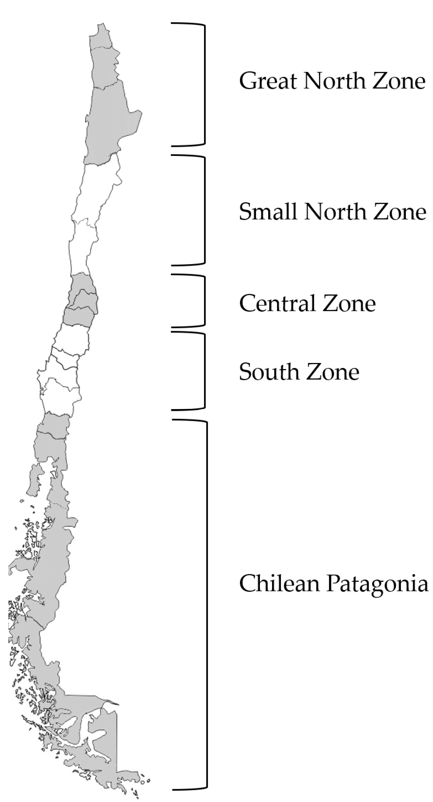
Figure 1. Share of agricultural employment and GPD in total agricultural activities. Source: Own elaboration with data from Central Bank of Chile and National Statistics Institute–Chile.
Agriculture 12 02110 g001
Figure 2. Map of Chile.
Agriculture 12 02110 g002
Figure 3. Distribution of agricultural employment and GDP in Chile, 2018. Source: Own elaboration with data from Central Bank of Chile and National Statistics Institute–Chile.
Agriculture 12 02110 g003
Figure 4. Share of agricultural employment and GPD in total activities by zone. Source: Own elaboration with data from Central Bank of Chile and National Statistics Institute–Chile.
Agriculture 12 02110 g004
Table 1. Main agrarian characteristic of macro-areas.
ZoneCharacteristics
Great North
  • This area accounts for 1.4% of the national crop area.
  • The most important crops in this area are vegetables, fruit trees, and fodder plants.
  • The level of livestock farming is low, mostly with llamas and rabbits.
Small North
  • This area accounts for 3.8% of the national surface area dedicated to crops.
  • Fruit crops and some fodder plants feature prominently in this area.
  • The area has a relatively high proportion of goats and rabbits compared with the rest of the country.
Central
  • This area accounts for 15.1% of the national crop area.
  • The most important crops in this area are fruit, vegetables, cereals, vines, and grapevines.
  • The level of livestock farming is low, although pig farming comparatively dominates in the southern part of the region.
South
  • This area accounts for 54.9% of the national surface area dedicated to crops.
  • In this area, forest plantations, fruit trees, fodder plants, vineyards, and grapevines feature.
  • The area is relatively important in terms of cattle, horses, and pigs.
Patagonia
  • This area accounts for 8.2% of the national area dedicated to crops.
  • The most important crops in this area are forage, forestry, and cereal plantations.
  • In the northern part of Patagonia, cattle breeding is important, while sheep farming is important in southern Patagonia.
Source: Own elaboration with information from the website of the Ministry of Agriculture—Chile www.minagri.gob.cl, accessed on 1 December 2022 [25].
Table 2. Description of the data sample. Agricultural worker sectors in Chile, by macro-area.
Variables
Commutant
(proportion)
Male (proportion)Age (mean)Primary Studies
(proportion)
Secondary
Studies (proportion)
Post-Secondary Studies
(proportion)
Household Head
(proportion)
Full-Time JobFormal Job (proportion)Observations
Total Country: ChileNon-Commutant0.00000.746646.34980.54750.37440.07800.57740.79000.544718987
Commutant1.00000.750641.87220.34450.46790.18760.50080.92430.68522798
Total Sample0.14970.747245.67960.51710.38840.09450.56590.81010.565721785
*********************
Great North ZoneNon-Commutant0.00000.777444.78010.49000.43540.07460.63460.68830.25741569
Commutant1.00000.795141.25930.23420.64400.12180.55120.93150.2201144
Total Sample0.10210.779244.42080.46380.45670.07950.62610.71310.25361713
****** *****
Small North ZoneNon-Commutant0.00000.741148.38190.58760.33970.07270.58270.76480.44002377
Commutant1.00000.807242.16460.35610.46150.18240.50130.84720.5797241
Total Sample0.14340.750647.49050.55440.35720.08840.57110.77660.46002618
*********************
Central ZoneNon-Commutant0.00000.752645.14550.48250.43030.08730.55500.85910.68464688
Commutant1.00000.720741.78000.34790.47150.18060.45270.91530.70871077
Total Sample0.18400.746744.52620.45770.43790.10450.53620.86950.68915765
*********************
South ZoneNon-Commutant0.00000.726746.89640.59070.34020.06910.57900.76610.49466190
Commutant1.00000.746642.06250.34540.45520.19940.52970.94710.7080913
Total Sample0.13830.729546.22770.55670.35610.08720.57220.79120.52417103
********************
Patagonia ZoneNon-Commutant0.00000.780446.80590.56110.35240.08650.59840.75660.53014163
Commutant1.00000.816041.57760.35020.45740.19230.55490.92580.7077423
Total Sample0.12340.784846.16090.53510.36540.09960.59300.77750.55204586
***********************
Source: Own elaboration. ***, **, * indicate significance at 1%, 5% and 10%, respectively.
Table 3. Logistic estimation result and marginal effects: Chile.
Dependent Variable (Commutant = 1)CoefficientMarginal EffectP > z
Sex (1 = male)0.12750.0143*
(0.0709)(0.0077)
Age−0.0088−0.0010***
(0.0024)(0.0002)
Secondary Studies (1 = yes)0.47450.0568***
(0.0674)(0.0084)
Post-Secondary Studies (1 = yes)1.12630.1768***
(0.0972)(0.0195)
Household Head (1 = yes)−0.1356−0.0157**
(0.0661)(0.0077)
Full-time job (1 = yes)0.93840.0877***
(0.1165)(0.0081)
Formal Sector (1 = yes)0.30950.0351***
(0.0626)(0.007)
Constant−2.7205
(0.1578)
Pseudo R20.0554
LR Chi2 (7)404.92
Prob > Chi20.0000 ***
Observations21,751
Source: Own elaboration. ***, **, * indicate significance at 1%, 5% and 10%, respectively. Standard errors are in parentheses.
Table 4. Logistic estimation result and marginal effects by area.
VariableGreat NorthSmall NorthCentralSouth Patagonia
Dependent Variable (Commutant = 1)Coef.Marginal EffectCoef.Marginal EffectCoef.Marginal EffectCoef.Marginal EffectCoef.Marginal Effect
Sex (1 = male)0.20040.01300.49230.0498 *0.00480.00070.15360.01470.21380.0189
(0.3201)(0.0197)(0.2564)(0.0233)(0.1209)(0.0175)(0.1081)(0.0100)(0.2012)(0.0168)
Age0.00120.0001−0.0132−0.0015 *−0.0061−0.0009−0.0070−0.0007 *−0.0186−0.0017 ***
(0.0098)(0.0006)(0.0074)(0.0008)(0.0043)(0.0006)(0.0038)(0.0003)(0.0054)(0.0005)
Secondary Studies (1 = yes)1.09780.0798 ***0.54440.0641 ***0.29430.0433 **0.61080.0647 ***0.38380.0372 **
(0.3370)(0.0243)(0.2000)(0.0244)(0.1192)(0.0178)(0.1041)(0.0119)(0.1567)(0.0157)
Post-Secondary Studies (1 = yes)1.22430.1292 *1.14590.1761 **0.93080.1674 ***1.37720.2050 ***0.96820.1215 ***
(0.5067)(0.0740)(0.3659)(0.0720)(0.1704)(0.0363)(0.1540)(0.0312)(0.2068)(0.0327)
Household Head (1 = yes)−0.4872−0.0351−0.1877−0.0210−0.2746−0.0401 **0.00760.00070.05720.0053
(0.3190)(0.0233)(0.2298)(0.0259)(0.1126)(0.0165)(0.1097)(0.0108)(0.1576)(0.0145)
Full-time Job (1 = yes)1.84640.0976 ***0.19770.02100.56580.0716 ***1.34540.1005 ***1.03580.0779 ***
(0.3479)(0.0165)(0.2757)(0.0280)(0.2139)(0.0226)(0.1744)(0.0090)(0.2389)(0.0142)
Formal Sector (1 = yes)−0.6447−0.0386 ***0.45820.0516 ***0.00290.0004 ***0.51370.0503 ***0.32950.0302 ***
(0.3101)(0.0170)(0.1915)(0.0222)(0.1133)(0.0164)(0.0981)(0.0094)(0.1541)(0.0138)
Constant−4.1943 −2.2268 −1.8459 −3.5467 −2.7259
(0.6875) (0.5026) (0.2777) (0.2505) (0.3454)
Pseudo R20.0975 0.0591 0.0282 0.0860 0.0638
LR Chi2 (7)37.84 36.92 64.81 252.01 85.80
Prob > Chi20.0000 0.0000 0.0000 0.0000 0.0000
Observations1709 2616 5754 7093 4579
Source: Own elaboration. ***, **, * indicates significance at 1%, 5%, and 10%, respectively. Standard errors are in parentheses.
Table 5. Average probabilities of agrarian workers to commute.
ChileZone
Great NorthSmall NorthCentralSouthPatagonia
Agrarian Worker0.15000.10240.14350.18430.13880.1235
Agrarian Worker: Male0.15070.10420.15440.17800.14210.1284
Agrarian Worker: Female0.14790.09600.11080.20300.12990.1057
Agrarian Worker: Primary Studies0.10000.05170.09220.14010.08610.0808
Agrarian Worker: Secondary Studies0.18070.14440.18540.19850.17740.1546
Agrarian Worker: Post-Secondary Studies0.29790.15700.29600.31870.31740.2386
Agrarian Worker: Household Head0.13270.09000.12590.15550.12850.1155
Agrarian Worker: Non-Household Head0.17260.12340.16700.21760.15260.1351
Agrarian Worker: Full-time Job0.17130.13390.15660.19410.16630.1471
Agrarian Worker: Part-time Job0.05970.02440.09800.11950.03500.0411
Agrarian Worker: Age under 460.18310.11940.18510.21130.17580.1588
Agrarian Worker: Age 46 or more0.11830.07960.10890.15540.10610.0915
Agrarian Worker: Formal Sector0.18180.08890.18100.19000.18740.1583
Agrarian Worker: Informal Sector0.10860.10700.11160.17190.08510.0806
Source: Own elaboration.
Table 6. Result data matching: Propensity Score Matching.
ChileZone
Great
North
Small
North
CentralSouthPatagonia
Coef. Coef. Coef. Coef. Coef. Coef.
Sex
(1 = male)
−0.0114 0.0284 −0.0014 −0.0581***0.0021 0.0342*
(0.0086) (0.0204) (0.0157) (0.0134) (0.0183) (0.0175)
Age 46 or more−0.0888***−0.0591***−0.0933***−0.0432***−0.0949***−0.0983***
(0.0049) (0.0160) (0.0121) (0.0108) (0.0085) (0.0111)
Primary Studies (1 = yes)−0.0882***−0.0316**−0.0780***−0.0692***−0.1081***−0.0943***
(0.0057) (0.0137) (0.0119) (0.0127) (0.0081) (0.0092)
Secondary Studies (1 = yes)0.0551***0.0319**0.0442***0.0622***0.0610***0.0469***
(0.0054) (0.0142) (0.0121) (0.0116) (0.0084) (0.0103)
Post-Secondary Studies (1 = yes)0.1367***0.0064**0.0976**0.1827***0.1538***0.0813***
(0.0121) (0.0340) (0.0418) (0.0249) (0.0220) (0.0229)
Household Head (1 = yes)−0.0438***−0.0219**−0.0517***−0.0471***−0.0289***−0.0551***
(0.0050) (0.0166) (0.0110) (0.0093) (0.0093) (0.0104)
Full-time Job (1 = yes)0.1448***0.0227**0.0813***0.1389***0.1697***0.1273***
(0.0068) (0.0171) (0.0148) (0.0306) (0.0160) (0.0130)
Formal Sector (1 = yes)0.0828***−0.0474***0.0361**0.0907***0.1126***0.0765***
(0.0057) (0.0155) (0.0145) (0.0137) (0.0089) (0.0099)
Source: Own elaboration. ***, **, * indicates significance at 1%, 5%, and 10%, respectively. Standard errors are in parentheses.
Publisher’s Note: MDPI stays neutral with regard to jurisdictional claims in published maps and institutional affiliations.

