Modeling the Agricultural Soil Landscape of Germany—A Data Science Approach Involving Spatially Allocated Functional Soil Process Units

Abstract

The national-scale evaluation and modeling of the impact of agricultural management and climate change on soils, crop growth, and the environment require soil information at a spatial resolution addressing individual agricultural fields. This manuscript presents a data science approach that agglomerates the soil parameter space into a limited number of functional soil process units (SPUs) that may be used to run agricultural process models. In fact, two unsupervised classification methods were developed to generate a multivariate 3D data product consisting of SPUs, each being defined by a multivariate parameter distribution along the depth profile from 0 to 100 cm. The two methods account for differences in variable types and distributions and involve genetic algorithm optimization to identify those SPUs with the lowest internal variability and maximum inter-unit difference with regards to both their soil characteristics and landscape setting. The high potential of the methods was demonstrated by applying them to the agricultural German soil landscape. The resulting data product consists of 20 SPUs. It has a 100 m raster resolution in the 2D mapping space, and its resolution along the depth profile is 1 cm. It includes the soil properties texture, stone content, bulk density, hydromorphic properties, total organic carbon content, and pH.

1. Introduction

Global food security, the protection of our groundwater resources, and our efforts to combat climate change largely depend on the sustainable use of soils. This concerns the strategic planning of an adequate crop rotation, the careful use of fertilizers, and the restricted use of pesticides. To maintain the soils’ high productivity, we need to provide crops with sufficient and easily accessible nutrients. However, the soils’ storage potential is limited. Surplus fertilizer contaminates valuable water resources when it percolates to the groundwater. It enhances global warming while released as greenhouse gases into the atmosphere. Furthermore, crops also require sufficient plant-available soil water resources in their respective development stages. Irrigation needs to be crop- and soil-specific but may not be the best solution as it restricts water for other uses. In consequence, it requires thoughtful planning of an adapted crop cycle involving drought-tolerant cultivars [1] and respective soil water management by alternative means [2,3].

All decisions and their consequences with regards to soil productivity and environmental impact ultimately depend on the soil characteristics on site. Accordingly, the national-scale evaluation and modeling of the impact of agricultural management and climate change on agricultural soils, yields, and the environment require information on the multivariate 3D soil parameter space at a spatial resolution addressing individual agricultural fields [4,5]. This concerns the assessment of the soils’ agricultural productivity [6] and the restrictions and required adaptations due to prolonged drought periods. Crop phenology models [7] and the evaluation and modeling of soil-related drought [8,9,10] and corresponding irrigation requirements [11] could be improved to a large extent by adequate soil information at a high spatial resolution. The same applies to the evaluation of the soils’ storage potential for soil organic carbon [12,13], the modeling of the complex processes causing the release of greenhouse gases to combat climate change [14], and the modeling of mitigation options to reduce nitrate pollution [15,16].

Running agricultural process models at national scale requires information about the multivariate 3D soil parameter space at a spatial resolution targeting individual agricultural fields. With a spatial resolution of 100 m, this already amounts to about 20 million raster cells for the agricultural soils of Germany. Process models require high computing capacities to run repeated simulations considering agricultural management and climate scenarios on this number of raster cells. Unfortunately, this also goes along with an unnecessarily high amount of energy consumption, counteracting our efforts to combat climate change. Hence, a creative data science approach is required to agglomerate the information contained in the raster cells to a limited number of spatially allocated functional soil process units (SPUs). This enables us to reduce the required resources without having to accept a lower spatial resolution.

One might argue why not rather use the spatial map units (SMUs) contained in conventional soil maps as SPUs? For Germany, there are mainly three reasons why the contained soil information is inappropriate: (1) The best conventional soil map available at national scale for Germany is the BÜK at a map scale of 1:250.000 [17]. Its SMUs each define a paragenesis of soil systematic units (SUs) with highly differing characteristics. The spatial allocation of these SUs within the SMUs is unknown. Hence, the contained information is not site-specific when it comes to addressing individual agricultural fields. (2) Important soil properties guiding soil functionality are only distinguished at a low hierarchical level of the German soil classification system KA [18]. Rather similar soils concerning their properties and functionality are assigned to different upper-level SUs. This particularly applies to the particle size distribution, which is one of the most important properties guiding soil functionality. (3) Last but not least, the BÜK is uncertain. All soil maps are. However, on the one hand, the BÜK’s uncertainty is unknown. On the other hand, its uncertainty likely differs between the federal states as the map was developed by slightly differing approaches at the regional soil survey institutions and then later joined and harmonized concerning inconsistencies at the regional boundaries.

The development of creative data science approaches to provide spatially continuous soil information relates to the research field pedometrics. Pedometrics is an interdisciplinary science that integrates soil science with geoinformatics and data science. Pedometric modeling approaches are used to investigate the spatial-temporal variation of the soil landscape and derive spatially continuous soil information from soil profile data. They rely on the conceptual model of pedogenesis, with soils and their vertical profile differentiation and characteristics being the product of the site-specific interaction of the soil-forming factors through long periods of time [19]. The conceptual approach was extended by McBratney et al. [20] to include geographic location and proxies for soil itself. The resulting SCORPAN factors include proxies to soil (S), climate (C), organisms including land use, agricultural management, etc. (O), relief (R), parent material (P), age (A), and geographic location (N). They are each approximated by spatially continuous gridded data proxies from either remote sensing, by conducting a digital terrain analysis, and/or by including expert knowledge. Padarian et al., Arrouays et al., and Chen et al. [21,22,23] provide recent reviews. Many studies refer to pedometric modeling for landscape-scale predictions by the terms ‘digital soil mapping’ or ‘predictive soil mapping’. I prefer the term pedometric modeling since digital soil maps are also created by other approaches, and any map is two-dimensional and, therefore, does not necessarily include 3D data products.

Current approaches in pedometric modeling to generate nationwide soil information predominantly address the prediction of individual soil properties. Žížala et al. and Gebauer et al. [24,25] provide recent 2D applications, Malone and Searle and Reddy et al. [26,27] 2.5D applications, and Padarian et al. and Ma et al. [28,29] 3D applications. However, the separate modeling of individual soil properties and their respective joint consideration as input to agricultural process models may result in constructed soil profile information that does not occur in reality and may be unrealistic according to the underlying pedogenetic processes and dependencies between the properties. Ließ et al. [4] provide a promising alternative for the joint modeling of multiple soil properties in 3D. The resulting data product represents the multivariate 3D soil parameter space of the nationwide agricultural landscape of Germany in terms of spatially allocated SPUs, each being described by a multivariate parameter distribution along the depth profile from 0 to 100 cm. It includes depth- and property-wise uncertainty estimates.

Here, a data science approach shall be developed that serves to generate such multivariate 3D data products consisting of spatially allocated functional SPUs. In contrast to Ließ et al. [4], it involves the development of unsupervised classification methods that account for differences in variable types and distributions and involve optimization to identify those SPUs with the lowest internal variability and maximum inter-unit difference with regards to both their soil characteristics and landscape setting. The approach shall be evaluated by applying it to the German agricultural soil landscape to improve the previously mentioned data product.

2. Materials and Methods

2.1. Data

2.1.1. Soil Profile Data—Consistency Check and Gap Filling

The soil profile data from the agricultural soil inventory of Germany [30] were used for this study. The data were collected by systematic sampling along an 8 km × 8 km grid at 3104 sites. Each soil profile has an identifier and geographic coordinates. The data comprise field data (dataF) in terms of a soil profile description according to the German soil survey system KA5 [18], and laboratory data (dataL). From dataF, the horizon-wise texture class, stone content, and the horizon symbol of all profiles were considered. From dataL, the particle-size distribution (3 particle-size separates), the bulk density, stone content, total organic carbon content (TOC), and the pH value of all profiles were considered. In the following, I describe the consistency check, subsequent data modification, and gap-filling procedure that were applied prior to any further analysis.

The sampling protocol for the Agricultural Soil Inventory states that samples for subsequent laboratory analysis ought to be taken for the depth increments 0–10, 10–30, 30–50, 50–70, and 70–100 cm while taking into account horizon boundaries, i.e., including multiple samples per depth increment for each corresponding soil horizon present with five or more centimeters [31]. However, as could be expected for such a large soil survey campaign involving multiple teams, the dataset contains some inconsistencies. To combine dataF and dataL, the two datasets were checked for mismatches in absolute profile depth and horizon sequence notation (term used for dataF and dataL), as well as non-compliant data entries, duplicates or gaps in the horizon sequence notation. After correcting non-compliant data entries, the next correction step concerned the mismatches in profile depth and horizon sequence notation. For their correction, I tested whether mismatches concerning depth and horizon sequence notation corresponded to additional layers (or horizons) and whether the difference was minor, up to 5 cm, i.e., mismatches in line with the sampling protocol. After adjusting the layer boundaries accordingly, all other mismatches were corrected stepwise by favoring the profile depth of dataF over dataL in case the difference was not caused by additional layers (or horizons), and by splitting layers of dataL if they included one or more horizon boundaries that differed from the upper or lower layer boundary by five or more centimeters. This procedure resulted in matching horizon sequence notation and profile depth between dataF and dataL, and the two datasets were combined using the profile identifier. From now on, these joint depth divisions will be referred to as horizons.

The modifications in the horizon sequence notation in dataL and dataF resulted in data gaps concerning all laboratory or field data of a certain depth interval. Further, using interpolation methods to fill these gaps may not be the best option due to the geological stratification, i.e., discontinuities in the soil profiles. In addition, the data gaps relating to the uppermost and last soil horizon cannot be filled in this way. Therefore, the following procedures were applied: The resulting texture data gaps in dataL were filled by additionally considering texture data from dataF. The mean value of the sand, silt and clay content (dataL) from other horizons with matching texture classes (dataF) was used. This happened stepwise. If the prerequisites were met, only data from the same profile were used. Otherwise the complete dataset’s respective class-wise mean values were assigned. Finally, the remaining texture classes were filled by the KA5 texture class’s mean sand, silt, and clay content. The latter corresponds to layers with uncommon soil texture classes and hence too few data entries (less than five). For data gaps in the TOC of organic soil horizons, a similar approach was followed considering horizon symbols and organic texture classes. For TOC in the mineral soil horizons, as well as the pH, bulk density and stone content of all horizons, random forest (RF) models were trained. Model training, tuning, and evaluation were conducted with nested stratified cross-validation (CV), as explained in Section 2.3.2. As predictors, the same property’s values from upper and lower horizons as well as related soil properties of over- and underlying horizons were used. Related properties of the same horizon could not be used unless for those where dataF was used to fill gaps in dataL.

After gap filling, some additional variables were created. For the stone content, the data from dataF and dataL were combined by assigning the maximum of the two values. This was done since on the one hand, dataL underestimates the stone content with regards to large rock fragments beyond the size of the steel cores used for sampling. On the other hand, the visual method applied to estimate the stone content in dataF may neglect smaller rock fragments. Concerning hydromorphic features, one variable was created for each, the presence (value = 1) or absence (value = 0) of stagnic and gleyig properties, and named symbol_S and symbol_G. The information was derived from the horizon symbology of dataF. An additional variable ‘mob’ was included in the dataset assigning each horizon to either ‘mineral’, ‘organic’, or ‘bedrock’ by considering the TOC, horizon symbology, and the availability of texture data. Each profile was then subdivided into 1 cm slices up to a depth of 100 cm.

2.1.2. Data Cube of Covariates

The covariates included to train and apply the machine learning models for nationwide spatial prediction were grouped according to the SCORPAN factor they represent. Table 1 gives an overview. Ließ et al. [4] provide a description of the German landscape setting.

Table 1. Covariates.

Soil Forming Factor	Abbreviation	Description	Data Source
Climate	PRESU	Average seasonal precipitation (summer) [raster, 1000 m]	[32]
	PREWI	Average seasonal precipitation (winter) [raster, 1000 m]
	TEMSU	Average seasonal temperature (summer) [raster, 1000 m]	[33]
	TEMWI	Average seasonal temperature (winter) [raster, 1000 m]
	DINSU	Average seasonal drought index (summer) [raster, 1000 m]	[34]
	DINWI	Average seasonal drought index (winter) [raster, 1000 m]
Organisms/Soil	B0118, 0218, …B0818, B8A18, B1118, B1218	Sentinel-2 spectral bands B1, B2, …B8, B8A, B11, and B12 composites of the 2nd yearly quartile of the year 2018
	B0121, 0221, …B0821, B8A21, B1121, B1221	Sentinel-2 spectral bands B1, B2, …B8, B8A, B11, and B12 composites of the 2nd yearly quartile of the year 2021
	EVI18, EVI21	Enhanced vegetation index, calculated from Sentinel 2 band composites of 2nd quartile 2018 & 2021 (S2-Q2-18/21), EVI = G ∗ (B8A − B04)/(B8A + C1 ∗ B04 − C2 ∗ B02 + L), with G = 2.5, C1 = 6, C2 = 7.5 and L = 1
	MSI18, MSI21	Moisture index: S2-Q2-18/21, MSI = B11/B08
	NDM18, NDM21	Normalized difference moisture index: S2-Q2-18/21, NDMI = (B08 − B11)/(B08 + B11)
	NDV18, NDV21	Normalized difference vegetation index: S2-Q2-18/21, NDVI = (B08 − B04)/(B08 + B04)
	NDW18, NDW21	Normalized difference water index: S2-Q2-18/21, NDWI = (B03 − B08)/(B03 + B08)
	PSR18, PSR21	Plant senescence reflectance index: S2-Q2-18/21, PSRI = (B04 − B02)/B06
	DMP16	Dry matter productivity, June 2016 [raster, 300 m]	[35]
	DMP18	Dry matter productivity, June 2018 [raster, 300]
	VPI16	Vegetation Productivity Index, June 2016 [raster, 300 m]	[36]
	VPI18	Vegetation Productivity Index, June 2018 [raster, 300 m]
Topography	GMK00	Geomorphographic map of Germany [raster, 250 m resolution, map scale 1:1,000,000]	[37]
	DEM00	Digital elevation model [raster, 25 m resolution]	[38]
	SLO01, SLO05, SLO10	Slope: calculated from DEM (cfD) with a search radius of 1, 5, 10 cells, using SAGA module Morphometric features
	NOR01, NOR05, NOR10	Northness: derived from aspect cfD with a search radius of 1, 5, 10 cells, using SAGA module Morphometric features
	EAS01, EAS05, EAS10	Eastness: derived from aspect cfD with a search radius of 1, 5, 10 cells, using SAGA module Morphometric features
	TST01, TST05, TST10	Terrain surface texture: cfD with a search radius of 1, 5, 10 cells, using SAGA module Terrain Surface Texture
	TSR01, TSR05, TSR10	Terrain surface ruggedness: cfD with a search radius of 1, 5, 10 cells, using SAGA module Terrain Ruggedness Index
	CON01, CON05, CON10	Convergence index: cfD with a search radius of 1, 5, 10 cells, using SAGA module Convergence Index (Search Radius)
	SLH00	Slope height: cfD using SAGA module Relative Heights and Slope Positions
	VAD00	Valley depth: cfD using SAGA module Relative Heights and Slope Positions
	NOH00	Normalized height: cfD using SAGA module Relative Heights and Slope Positions
	WIN00	Wind exposure: cfD using SAGA module Wind Effect
	NOP00	Negative openness: cfD using SAGA module Topographic Openness
	POP00	Positive openness: cfD using SAGA module Topographic Openness
	VOF0S	Vertical overland flow distance to all river segments: cfD using SAGA module Terrain analysis/Channels
	VOF0M	Vertical overland flow distance to major rivers: cfD using SAGA module Terrain analysis/Channels
	HOF0S	Horizontal overland flow distance to all river segments: cfD using SAGA module Terrain analysis/Channels
	HOFOM	Horizontal overland flow distance to major rivers: cfD using SAGA module Terrain analysis/Channels
	SWI00	SAGA wetness index: cfD using SAGA module SAGA Wetness Index
Parent material	LIT00	Lithology, Hydrogeological map of Germany, HÜK [polygon shapefile, map scale 1:250,000]	[39]
	STR00	Stratigraphy, Hydrogeological map of Germany, HÜK [polygon shapefile, map scale 1:250,000]
	BAG00	Groups of soil parent material in Germany [polygon shapefile, map scale 1:5,000,000]	[40]
Soil	BGL00	Soil scapes in Germany [map scale 1:5,000,000]	[41]
	DMP86	Dry matter productivity, DMP18–DMP16 [raster, 300 m]
	VPI86	Vegetation Productivity Index, VPI18–VPI16 [raster, 300 m]
Geographic location	LAT00	INSPIRE Latitude	[42]
	LON00	INSPIRE Longitude

Table 1. Covariates.

Soil Forming Factor	Abbreviation	Description	Data Source
Climate	PRESU	Average seasonal precipitation (summer) [raster, 1000 m]	[32]
	PREWI	Average seasonal precipitation (winter) [raster, 1000 m]
	TEMSU	Average seasonal temperature (summer) [raster, 1000 m]	[33]
	TEMWI	Average seasonal temperature (winter) [raster, 1000 m]
	DINSU	Average seasonal drought index (summer) [raster, 1000 m]	[34]
	DINWI	Average seasonal drought index (winter) [raster, 1000 m]
Organisms/Soil	B0118, 0218, …B0818, B8A18, B1118, B1218	Sentinel-2 spectral bands B1, B2, …B8, B8A, B11, and B12 composites of the 2nd yearly quartile of the year 2018
	B0121, 0221, …B0821, B8A21, B1121, B1221	Sentinel-2 spectral bands B1, B2, …B8, B8A, B11, and B12 composites of the 2nd yearly quartile of the year 2021
	EVI18, EVI21	Enhanced vegetation index, calculated from Sentinel 2 band composites of 2nd quartile 2018 & 2021 (S2-Q2-18/21), EVI = G ∗ (B8A − B04)/(B8A + C1 ∗ B04 − C2 ∗ B02 + L), with G = 2.5, C1 = 6, C2 = 7.5 and L = 1
	MSI18, MSI21	Moisture index: S2-Q2-18/21, MSI = B11/B08
	NDM18, NDM21	Normalized difference moisture index: S2-Q2-18/21, NDMI = (B08 − B11)/(B08 + B11)
	NDV18, NDV21	Normalized difference vegetation index: S2-Q2-18/21, NDVI = (B08 − B04)/(B08 + B04)
	NDW18, NDW21	Normalized difference water index: S2-Q2-18/21, NDWI = (B03 − B08)/(B03 + B08)
	PSR18, PSR21	Plant senescence reflectance index: S2-Q2-18/21, PSRI = (B04 − B02)/B06
	DMP16	Dry matter productivity, June 2016 [raster, 300 m]	[35]
	DMP18	Dry matter productivity, June 2018 [raster, 300]
	VPI16	Vegetation Productivity Index, June 2016 [raster, 300 m]	[36]
	VPI18	Vegetation Productivity Index, June 2018 [raster, 300 m]
Topography	GMK00	Geomorphographic map of Germany [raster, 250 m resolution, map scale 1:1,000,000]	[37]
	DEM00	Digital elevation model [raster, 25 m resolution]	[38]
	SLO01, SLO05, SLO10	Slope: calculated from DEM (cfD) with a search radius of 1, 5, 10 cells, using SAGA module Morphometric features
	NOR01, NOR05, NOR10	Northness: derived from aspect cfD with a search radius of 1, 5, 10 cells, using SAGA module Morphometric features
	EAS01, EAS05, EAS10	Eastness: derived from aspect cfD with a search radius of 1, 5, 10 cells, using SAGA module Morphometric features
	TST01, TST05, TST10	Terrain surface texture: cfD with a search radius of 1, 5, 10 cells, using SAGA module Terrain Surface Texture
	TSR01, TSR05, TSR10	Terrain surface ruggedness: cfD with a search radius of 1, 5, 10 cells, using SAGA module Terrain Ruggedness Index
	CON01, CON05, CON10	Convergence index: cfD with a search radius of 1, 5, 10 cells, using SAGA module Convergence Index (Search Radius)
	SLH00	Slope height: cfD using SAGA module Relative Heights and Slope Positions
	VAD00	Valley depth: cfD using SAGA module Relative Heights and Slope Positions
	NOH00	Normalized height: cfD using SAGA module Relative Heights and Slope Positions
	WIN00	Wind exposure: cfD using SAGA module Wind Effect
	NOP00	Negative openness: cfD using SAGA module Topographic Openness
	POP00	Positive openness: cfD using SAGA module Topographic Openness
	VOF0S	Vertical overland flow distance to all river segments: cfD using SAGA module Terrain analysis/Channels
	VOF0M	Vertical overland flow distance to major rivers: cfD using SAGA module Terrain analysis/Channels
	HOF0S	Horizontal overland flow distance to all river segments: cfD using SAGA module Terrain analysis/Channels
	HOFOM	Horizontal overland flow distance to major rivers: cfD using SAGA module Terrain analysis/Channels
	SWI00	SAGA wetness index: cfD using SAGA module SAGA Wetness Index
Parent material	LIT00	Lithology, Hydrogeological map of Germany, HÜK [polygon shapefile, map scale 1:250,000]	[39]
	STR00	Stratigraphy, Hydrogeological map of Germany, HÜK [polygon shapefile, map scale 1:250,000]
	BAG00	Groups of soil parent material in Germany [polygon shapefile, map scale 1:5,000,000]	[40]
Soil	BGL00	Soil scapes in Germany [map scale 1:5,000,000]	[41]
	DMP86	Dry matter productivity, DMP18–DMP16 [raster, 300 m]
	VPI86	Vegetation Productivity Index, VPI18–VPI16 [raster, 300 m]
Geographic location	LAT00	INSPIRE Latitude	[42]
	LON00	INSPIRE Longitude

Concerning SCORPAN C, seasonal averages of air temperature and drought and the sum of precipitation of the winter (Dec., Jan., and Feb.) and the summer (Jun., Jul., and Aug.) months were derived from the German Weather Service (DWD). The seasonal averages of the drought index were calculated from DWD temperature in degrees centigrade (T) and precipitation in millimeters (P) grids as P/(T + 10).

To approximate SCORPAN O, the following covariates were included: Sentinel-2 data composites of the second yearly quartile of 2018 and 2021 of the bands B01, B02, B03, B04, B05, B06, B07, B08, B8a, B11, and B12, as well as the vegetation indices EVI, MSI, NDMI, NDVI, NDWI, and PSRI (please see Table 1 for the details). The composites were compiled using the Sentinel-Hub on behalf of the surface reflectance values, from the Level 2A product. The composites were downloaded as multiple tiles in 20 m spatial resolution, then mosaicked and resampled to the 100 m Infrastructure for Spatial Information in Europe (INSPIRE) grid topology [42] before calculating the vegetation indices. Additionally, remote sensing products on dry matter productivity (DMP) and the Vegetation Productivity Index (VPI) of the time slot June 11th–20th of the years 2016 and 2018 were derived from the Copernicus Global Land Service. All SCORPAN O covariates seek to capture the main annual phase of agricultural productivity.

SCORPAN R was represented by the geomorphographic map of Germany and terrain parameters derived by digital terrain analysis with the System for Automated Geoscientific Analyses (SAGA) [43] from the EU–DEM digital elevation model.

The map of the “Groups of soil parent material” was included to approximate SCORPAN P. Lithology and stratigraphy according to the hydrogeological map of Germany were additionally incorporated.

Proxies to soil itself (SCORPAN S) can generally be included in the form of conventional soil polygon maps, and remote sensing products relating to soil properties. Regarding the former, the map of the German soil scapes was included. Concerning the latter, differences in DMP and VPI between the dry year 2018 and the rather wet year 2016 were included. They relate to crop phenology affected by drought and, therefore, to the root zone plant-available soil water capacity.

All covariates were resampled to the INSPIRE grid topology at 100 m resolution [42]. This resolution was chosen as a compromise between the ambition to provide soil information for individual agricultural fields and a restrictive use of computing capacities. The nearest-neighbor method was used for categorical predictors, and B-spline interpolation was applied for numeric predictors. INSPIRE latitude and longitude were additionally included to represent the geographic location (SCORPAN N), and particularly to represent spatial patterns not captured by the other data proxies. The national border and coastline of Germany were derived from the digital land model at map scale of 1:250,000 (version 2.0) provided by the Federal Agency for Cartography and Geodesy (^©GeoBasis-DE/BKG, 2020).

2.2. Differentiation of Functional SPUs

The nationwide data product is composed of a limited number of spatially allocated functional SPUs, each being defined by a multivariate parameter distribution along the depth profile. Each SPU’s internal variability is described by a probability density distribution of all considered soil properties in all 1 cm depth slices. Two data science approaches were developed to derive SPUs with the lowest possible internal variability and maximum inter-unit difference with regards to both their soil characteristics and landscape setting. They are unsupervised classification methods, rely on the partitioning-around-medoids (PAM) algorithm [44] and involve optimization. Furthermore, they address the major concern that the joint consideration of mixed variable types (categorical and numerical) and variables of different distribution and scale have on the clustering result. Ahmad and Khan [45] and Van Mechelen et al. [46] provide an overview. In this particular case, there are variables with 1–0 coding for presence–absence type variables (symbol_S, symbol_G), variables with many zero values (stone content), variables with a threefold distribution (texture represented by sand, silt, and clay content), and variables with a bimodal distribution (TOC, bulk density) due to the inclusion of profiles that are all-mineral and profiles composed of mineral and organic horizons. PAM clustering after a mere data transformation did not yield satisfying results.

The two approaches will be described in the following sections. However, two aspects concern the methodology of both approaches:

• The gap-filled, sliced (1 cm slices) profile data were used to calculate individual property distance matrices. First, the data were normalized to a range between 0 and 1, considering all slices in all profiles except for texture. For texture, the composites’ relation of sand, silt, and clay content were kept summing up to 1. Then, the mean of the slice-wise Euclidian profile distance was calculated for each variable and stored in separate distance matrices. Non-defined distances in case of differences in soil material causing missing data, e.g., missing texture data for organic horizons or slices assigned to bedrock, were assigned the maximum distance occurring between any two profile slices for the respective soil property. These property-wise distance matrices were then again normalized, resulting in a minimum distance of 0 and a maximum distance of 1. Hereafter, they will be referred to as normalized single-property distance matrices (nSPdist).
• The respective input parameter vectors of the involved optimization process to extract the SPUs are evaluated on behalf of a complex objective function. It seeks to identify those SPUs with the lowest possible internal variability and maximum inter-unit difference with regards to both their soil characteristics and landscape setting. The former is evaluated by using the Silhouette Index [47]. The latter requires the training of machine learning models to capture the soil-landscape relation and evaluate their predictive performance. A simple and fast learner is required to reduce the required computation time. The random forest (RF) algorithm [48] was chosen to suit this purpose. It is described in Section 2.3.1.

2.2.1. Approach 1 (PAMp)—SPU Extraction by P Weights Optimization

Approach 1 seeks to obtain the optimal SPUs in terms of the lowest property-wise predictive RMSE from pedometric model training by simultaneously optimizing the number of clusters nclus and the weights Pw₁, Pw₂, Pw₃, …, Pw_p (p = number of soil properties) applied to the nSPdist. The weights give the inter-profile distances with regards to certain soil properties higher or lower importance compared to others. To avoid confusion, the weights will hereafter be termed P weights (property weights). Approach 1 will, therefore, be named PAMp. The objective function evaluated for each of the number of n parameter vectors of z = 8 components (seven P weights and nclus) evaluated in each iteration step of the optimization is shown in Figure 1. It consists of the following parts:

1.

Pw₁, Pw₂, Pw₃, …, Pw_p in the range [0.1, 1] are assigned to each nSPdist, which are then combined by calculating the weighted average (dist). The values of the resulting distance matrix are normalized to the range [0, 1].

2.

PAM clustering is conducted on the normalized distance matrix (ndist) with nclus = 8, 9, …, 100. The nclus minimum value was selected according to Ließ et al. [4]. For each input parameter vector including Pw₁, Pw₂, Pw₃, …, Pw_p and $nclus$, the best cluster solution is selected on behalf of the Silhouette Index.

3.1.

The resulting clustering solution Rdata_in, which assigns each soil profile to one cluster, is then combined with the respective l covariates’ values x₁, x₂, …, x_l of each profile (Pdata) to compile the predictor-response dataset (PRdata). The data were subdivided into 5 folds for a stratified 5-fold CV (Section 2.3.2). Categorical covariate values with zero data instances in any of the folds were removed.

3.2.

Each profile’s property-wise mean along the depth profile, Rdata_in [y₁, y₂, …, y_p], was used to compute property-wise means per cluster.

4.

An RF model was trained by 5-fold stratified CV using the PRdata [3.1] as input. The function ‘rfsrc’ of R package ‘randomForestSRC’ [49] was used with 1000 trees, a node size of five, and the default setting for the mtry parameter, while imputing no data values.

5.1.

The previously computed property-wise cluster means [3.2] were assigned to each profile on behalf of the test set RF predictions (Rdata_pred) generating Rdata_pred [y₁, y₂, …, y_p].

5.2.

The property-wise RMSE was calculated using Rdata_in [y₁, y₂, …, y_p] and Rdata_pred [y₁, y₂, …, y_p]. The objective function value corresponds to the negative mean of the property-wise RMSE values. It is maximized in the optimization process.

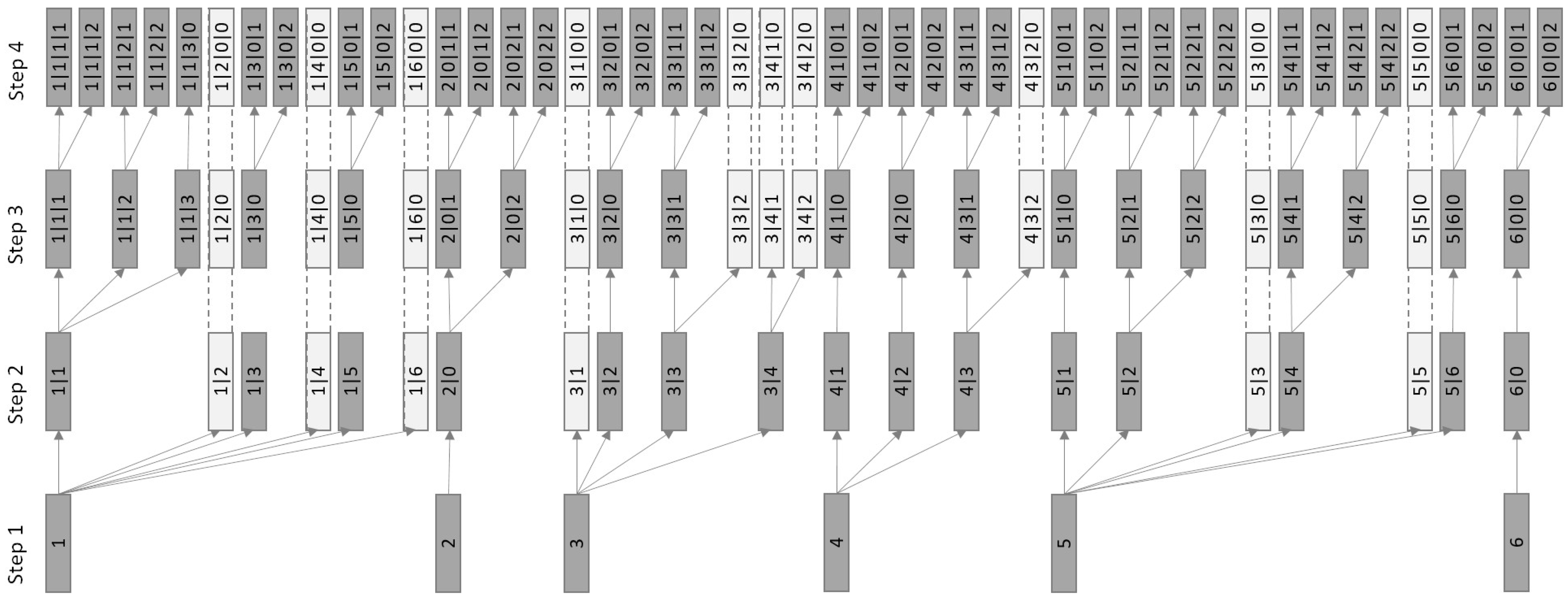
2.2.2. Approach 2 (PAMm)—SPU Extraction by Optimized Multistep Clustering

Approach 2 seeks to obtain the optimal SPUs in terms of the lowest property-wise predictive RMSE from pedometric model training by applying a multistep clustering with PAM. It will, therefore, be termed PAMm. In this approach, Part 1 and Part 2 of the objective function of PAMp are replaced by the multistep approach (Figure 2). The other subsequent parts remain the same.

The properties considered at each step need to be selected in advance. Optimizing their selection would have increased the complexity of the optimization task and hence required more iterations before convergence. Multistep clustering was conducted in the following way: Step 1 (texture), Step 2 (symbol_S, symbol_G), Step 3 (stone content, bulk density), and Step 4 (TOC, pH). The normalized distance matrices ndist_1, ndist₂, ndist₃, and ndist₄ for each step were prepared in advance and then provided as input to the objective function. Each ndist was calculated as the normalized average of the nSPdist of the soil properties considered in the respective step.

In Step 1, PAM is applied to ndist₁ testing a number of 2 to ncl_u clusters. The cluster solution with the best Silhouette Index value is chosen unless there are cluster solutions with a sufficiently good Silhouette Index value equal to or above the threshold sil₁. In that case, the cluster solution with the maximum number of clusters from all cluster solutions with a Silhouette Index value greater than or equal to sil₁ is chosen. In Step 2, PAM is conducted for each cluster resulting from Step 1. This requires subsetting ndist₂ according to the profile IDs that were assigned to the respective higher-level Step 1 clusters cl₁, cl₂, … and normalizing the distance matrix subsets, which were then named $n{d}_{cl1}$, $n{d}_{cl2}$, etc. The clusters resulting from Step 2 receive a 2nd cluster identifier, e. g., cl_1|1, cl_1|2, cL_2|1, cl_2|2 indicate that the two clusters from Step 1 were each subdivided into two clusters in Step 2. This procedure is repeated likewise for Step 3 and Step 4.

In order not to force unreasonable splitting into a high number of clusters supported by only a low number of profiles, two criteria are tested after each step: (1) The Silhouette Index value of the nd_z cluster solution needs to be greater than or equal to the threshold value sil_min, and (2) the number of profiles in each resulting cluster from nd_z needs to have a minimum number of profiles p_min. If any of the criteria are not fulfilled, then no subdivision is conducted for the respective higher-level cluster in this step, and all profiles receive the identifier 0. p_min is also considered to check whether the upper parameter limit of ncl_u needs to be reduced before running PAM on nd_z. PAM is run in parallel for the respective profile subsets starting from Step 2. A stopping criterion is included to stop in case Step 2 or Step 3 leads to an overall number of clusters nclus of 100 or more. Seven parameters were optimized in PAMm:

• ncl_u: The maximum number of clusters considered in each step.
• sil_1,2,3,4: One Silhouette Index threshold value per step.
• sil_min: The minimum Silhouette Index value tolerated to accept a lower-level clustering solution.
• p_min: The minimum number of profiles per cluster.

Table 2. Parameter ranges for SPU differentiation by Approach 2.

Parameter	Lower Limit	Upper Limit
nclu	3	10
sil1,	0.3	0.4
sil2,3,4	0.4	0.8
silmin	0.25	0.4
pmin	5	10

displays the respective parameter ranges. The ranges were chosen according to some test runs.

2.3. Modeling

The multivariate parameter distributions of the SPUs obtained by PAMp and PAMm are defined by the respective groups of assigned soil profiles. To regionalize the SPUs to the continuous space and to further enhance the extraction of the already-considered soil-landscape relation, two machine learning models were trained for each of the PAMp and PAMm results using the RF algorithm and the support vector machine (SVM) algorithm. Thus, model training by machine learning was applied for three scopes:

• for gap filling,
• for SPU differentiation, and
• to train the pedometric model fathoming the soil–landscape relation to obtain nationwide and spatially continuous predictions (regionalization task).

2.3.1. Machine Learning Algorithms

The RF algorithm [48] was applied for all three scopes. It is a recursive partitioning method. Depending on the supervised learning task at hand, it grows either multiple regression or classification trees. The results of all trees are averaged. In each tree, the data are subsequently partitioned by the predictor variables into preferably homogeneous subsets regarding the response variable. The mean of each data subset (regression task) or the dominating class (classification task) is then used as the predicted response value. A partition gateway is defined by the predictor and the threshold value in its range, which achieves the most homogeneous partition into two subsets (tree branches). Overall, the stability of the tree ensemble is obtained by training each tree model with a data subset and by using a subset of all predictors. RF is known to achieve reasonable results without tuning, an important characteristic to make it the perfect choice to act as the simple and fast learner for the objective function of the optimization task for Scope (2).

The function ‘cforest’ of R package ‘party’, an RF implementation employing conditional inference trees as base learners [50], was used to train the models for gap filling. Model training involved 500 trees (training 1000 trees did not improve model performance in this particular case). The size of the predictor subset (mtry) was tuned via a one-dimensional grid search including one to all predictors. The function ‘rfsrc’ of R package ‘randomForestSRC’ [49] was used for the tasks of Scopes (2) and (3). It provides a fast parallel computing implementation of RF. In both cases, 1000 trees were trained. However, while for Scopes (1) and (3) the mtry parameter was tuned, for Scope (2), the mtry parameter was set to the default to speed up computation time, i.e., use RF as a fast and simple learner.

The SVM algorithm [51] was applied for the regionalization task (Scope (3)) and compared to the RF models. While RF was applied to pay tribute to the fact that the optimization might have favored an SPU differentiation whose soil–landscape relation is well captured with RF (learner in the objective function), the SVM algorithm was chosen as a powerful algorithm, which led to promising results when capturing the soil–landscape relation to generate the data product of Ließ et al. [4].

SVMs were developed by Cortes and Vapnik [51]. In binary classification tasks, they search for the hyperplane that maximizes the margin between the two classes’ closest points. The properties of this decision surface ensure the SVM’s high generalization ability. Points along the boundary are called support vectors. The data are projected to the higher dimensional space via kernel techniques to allow for separation in case of nonlinearity. The radial basis function kernel was applied for this purpose. It helps to build complex decision boundaries and includes two parameters: C and γ, which need to be tuned. The γ parameter can be interpreted as the inverse of the radius of influence of the support vectors. C is the cost or penalty parameter. With a small C, the penalty for misclassified points is low; high values increase the risk of overfitting. Finally, it balances the misclassification of training samples against the simplicity of the hyperplane. R package “e1071” provides the R interface to the LIBSVM library for SVM [52,53]. To allow for multi-class classification, it uses the one-against-one technique by fitting all binary classifiers and finding the correct class by a voting mechanism. The two-dimensional parameter space to search for the optimal parameter combination expands in the following ranges: C [0.01, 100], γ [0.01, 10].

2.3.2. Model Training, Tuning, and Evaluation

For the gap-filling task, the predictor-response dataset consists of horizon-wise data (horizon sequence notation after combining dataL and dataF). For the SPU differentiation and regionalization tasks, it consists of profile-wise data. All numerical predictors were scaled to the range 0, 1 to avoid misbalance. Categorical data were kept for RF and recoded into dummy variables for SVM. To generate the predictor-response dataset for Scopes (2) and (3), the predictor values were extracted at the soil profile sites, and each soil profile was assigned to an SPU. Concerning SPU differentiation, the latter was performed in each iteration step of the objective function, as explained in Figure 1. Concerning the regionalization task, the final SPUs obtained respectively by PAMp and PAMm were used.

Model training and evaluation were conducted by a 5-times repeated 5-fold stratified CV [54] to obtain robust models. For the machine learning applications (Scope (1) and Scope (3)) involving model tuning via grid search (RF) or optimization (SVM), the CV was nested. The predictor-response dataset was subdivided into five folds of equal size using the response variable for stratification. Of these five folds, then always one fold was kept out as a test set while the other four were combined to form the model training set, leading to five separate test set evaluations (one per data instance). Each of the outer CVs’ training sets was again subdivided to provide the datasets for parameter tuning in the inner CV cycle. Concerning the categorical predictors, categories not present in all data subsets were removed before model training, tuning, and evaluation. To evaluate model performance, the test set predictions were compared to the measured data to calculate the slice-wise RMSE for each of the considered soil properties. The interquartile ranges of the SPUs’ multivariate distributions were used for this purpose, i.e., for each considered soil property and depth slice, it was tested whether the test set profile measurements fall within the interquartile range of the slice- and property-wise density distributions of the predicted SPU (residual of zero), whether they are smaller than the 25% quantile and how much (positive residual), or whether they are larger than the 75% quantile (negative residual). The five repetitions of the 5-fold CV resulted in 25 models and five RMSE values.

For the RF models to conduct gap-filling, a repeated 5-fold stratified group CV was applied, i.e., all horizons of a profile were assigned to the same fold to avoid overoptimistic test set estimates due to spatial autocorrelation. Concerning the regionalization task with SVM, the parameter tuning involving optimization was in a first step only conducted on behalf of one out of the 25 training sets of the outer CV cycle to check whether this provided satisfying results, while the obtained tuning parameter values were applied to all other training sets. Altogether, for the regionalization with RF and SVM of the SPUs obtained by PAMp and PAMm, four pedometric models were trained. They will be referred to as RF–PAMp, RF–PAMm, SVM–PAMp, and SVM–PAMm.

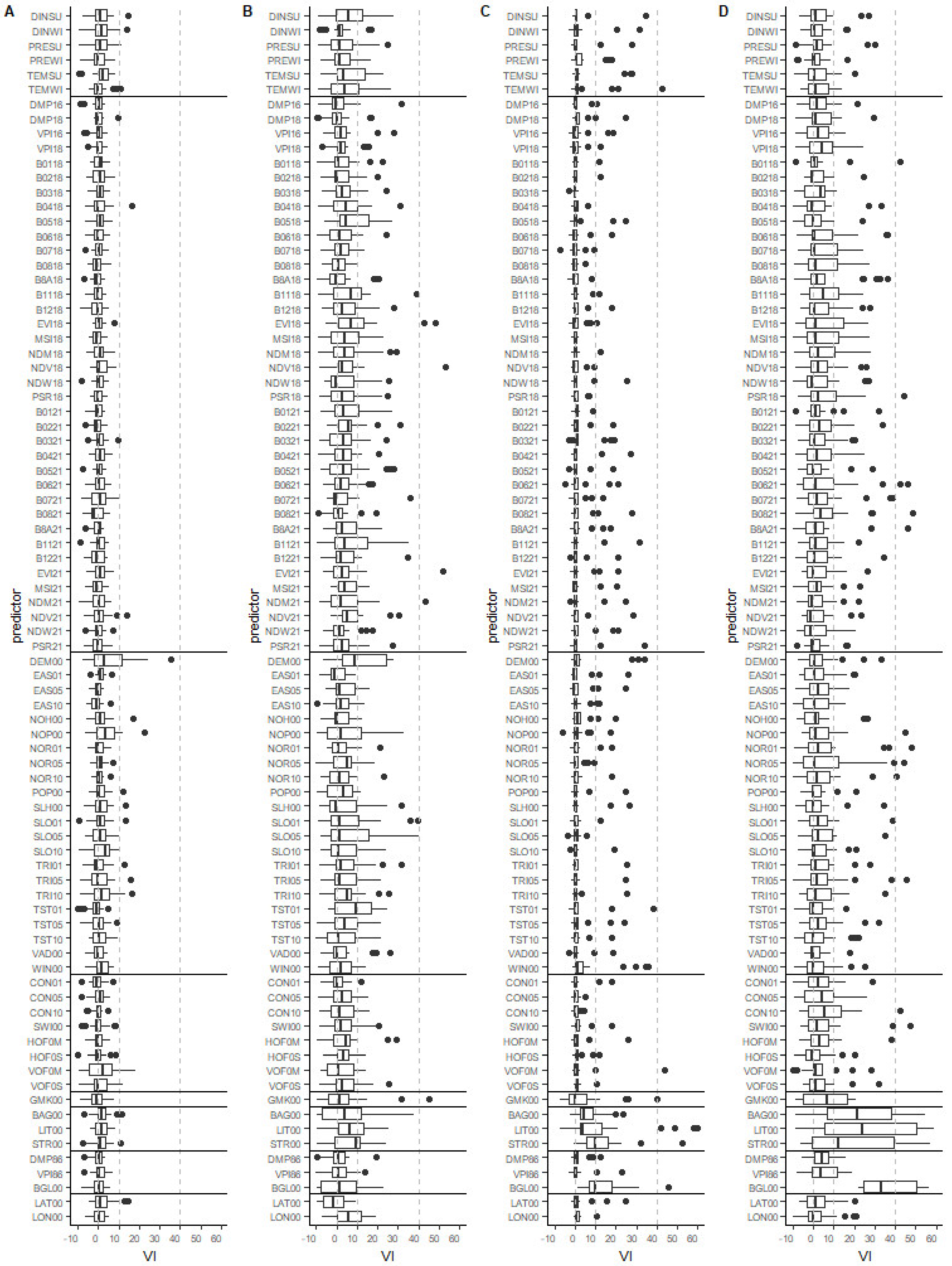
2.3.3. Variable Importance

Concerning gap filling (Scope (1)) with cforest, the package’s internal variable importance (VI) measures were used. Concerning the regionalization task (Scope (3)), a different procedure was followed to allow for the comparison between SVM and RF. For model interpretation, each predictor’s importance was obtained by permuting the predictor in the test set before model application. In this way, any predictor-response relationship with regards to that predictor was eliminated. The resulting relative decrease in model performance was then attributed as vVI to the respective predictor. Values of five permutations were averaged. The VI values for the dummy variables created from each of the categorical predictors (SVM) were summed. Due to the five times repeated 5-fold CV approach (outer CV cycle), the VI plots display boxplots of 25 VI values for each predictor.

2.4. Genetic Algorithm Optimization

Genetic algorithm (GA) optimization was applied to differentiate the SPUs (Scope (2)) and to conduct parameter tuning in machine learning (Scope (3)). The GAs’ operational structure is inspired by the general principles of biological evolution involving mutation, crossover, selection, and elitism [55]. The objective function for Scope (2) was described in Section 2.2 (Figure 1 and Figure 2). The objective function for SVM parameter tuning (Scope (3)) was defined as indicated by Figure 1, Parts 3–5 while replacing Part 4 with SVM. It corresponds to the inner CV cycle (Section 2.3.2). RF (Scope (1) and Scope (3)) does not require optimization for parameter tuning [4].

The parameter space to be searched for the optimal combination of parameter values had to be predefined by providing a minimum and maximum value for each parameter. Then, a random number of n parameter vectors, the parent population, was evaluated by a problem-specific objective function. Weights were assigned to each parameter vector according to its objective function value before starting to modify them by conducting ‘selection’, ‘mutation’ and ‘crossover’ to form a new population of parameter vectors, which was again evaluated. This process was iterated until either (1) an initially defined objective function value was achieved by any of the vectors, (2) a maximum number of iterations was reached, or (3) the overall best objective function value did not improve for a certain number of consecutive iterations. GA optimization was run in parallel, subdividing the parent population of size 500 into subpopulations and allowing for limited exchange of population individuals (parameter vectors) between the so-defined islands. Twenty-five islands (20 parameter vectors per island) were used for the differentiation of the SPUs with PAMp (Scope (2)) and the tuning of the SVM models (Scope (3)). For the differentiation of the SPUs with PAMm (Scope (2)), the number of islands was reduced to 5, resulting in a subpopulation size of 100 per island. The search on the islands was not run in parallel but sequentially due to conflicts that were otherwise caused by the parallelization of the objective function.

3. Results and Discussion

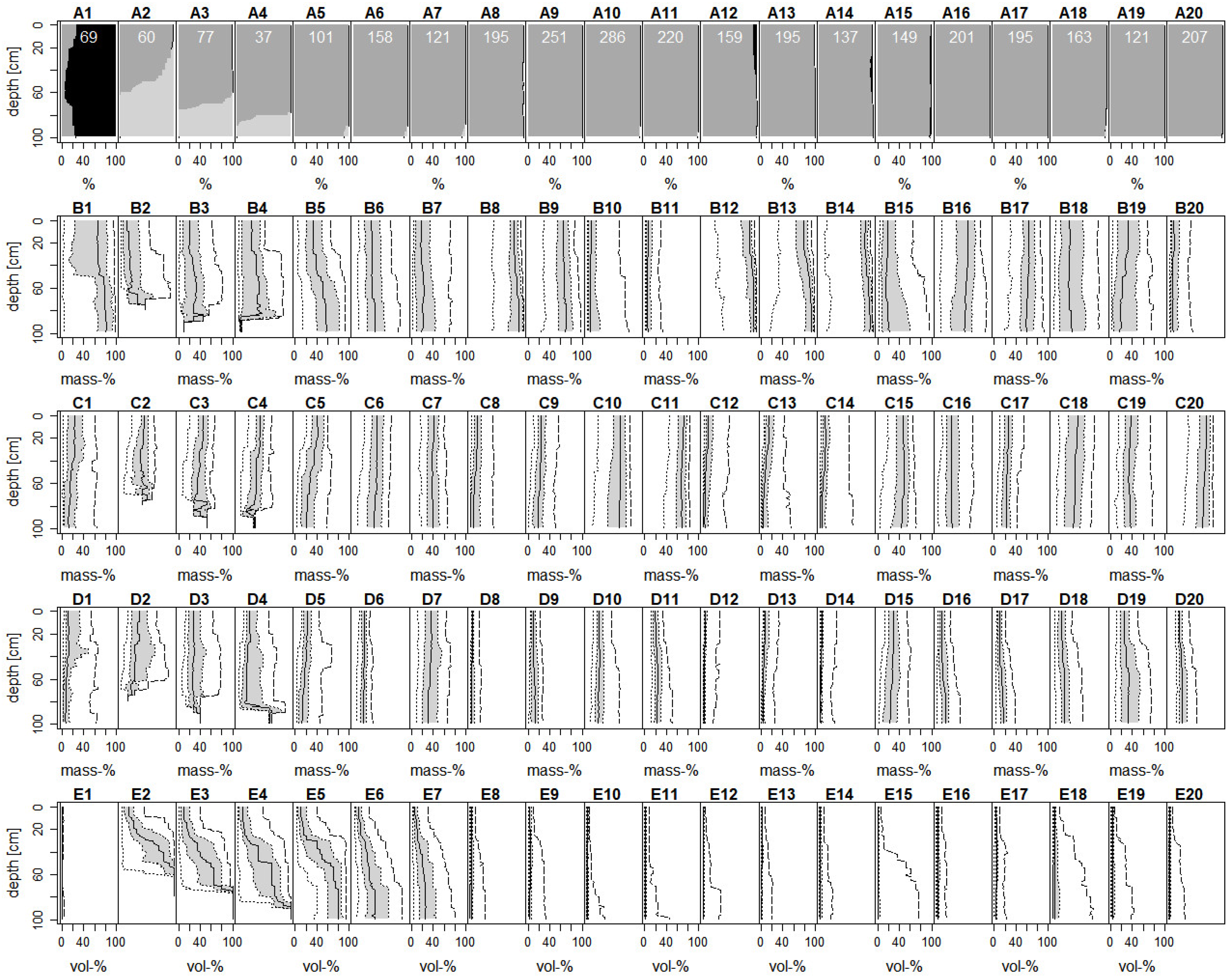
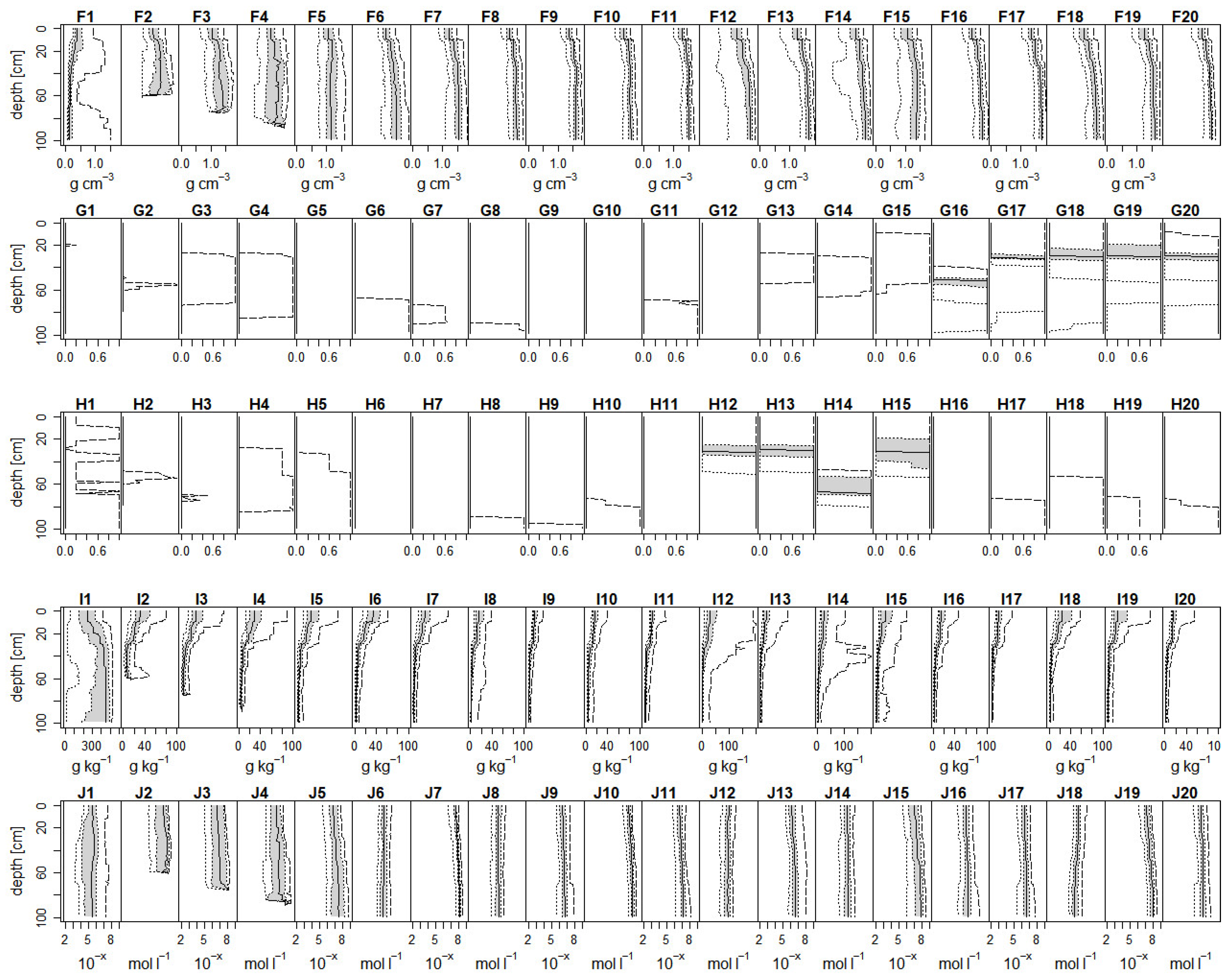
3.1. Gap Filling

Gap-filling of the soil profile data was needed to calculate the slice-wise distance matrices and run PAMp and PAMm. The gaps originated from the correction for horizon sequence notation mismatches between dataL and dataF. With an average R² between 0.86 and 0.95, all gap-filling models displayed very good predictive performance (Figure 3B). The RMSE amounted to a mean value of 0.12 g cm⁻³ for bulk density, 5.9 Vol-% for stonesF, 3.7 Vol-% for stonesL, 5.9 g kg⁻¹ for TOC, and 0.22 for pH (Figure 3A1–A4). The respective gap-filling of dataL with dataF for the particle size distribution and TOC of organic horizons remains unevaluated. It consists of the consideration of field estimates for those depth increments where laboratory data is missing, a common practice in soil science. The data are of course less precise since the KA5 soil survey instructions identify property classes instead of precise values. Errors in the class assignment were corrected by the approach presented here.

Data gaps in soil profile data are a common feature. Multiple approaches have been applied, including extrapolation to estimate soil properties in deeper soil horizons, gap-filling to provide estimates on behalf of expert knowledge, or assigning values from associated databases [56,57]. I am unaware, though, of any other publication documenting the use of multiple soil properties from over- and underlying horizons to train machine learning models to conduct gap filling. However, machine learning algorithms are readily applied to fill spatial data gaps in remote sensing data [58,59] and temporal gaps in time series data [60,61]. Another related field is the development of pedotransfer functions to estimate missing data of soil properties that are laborious to determine from other, readily available properties using machine learning. Ghanbarian and Pachepsky [62] provide a review.

Figure 4 displays the relative VI values for the respective gap-filling models for bulk density (Figure 4a), stonesL (Figure 4b), stonesF (Figure 4c), TOC (Figure 4d), and pH (Figure 4e). The minimum and maximum profile values, the horizon’s material, the horizon’s sand and silt content, as well as the underlying horizon’s TOC value, were the most important predictors for gap-filling bulk density data. The stonesF data were gap-filled detecting the horizon’s dataL stone content, the horizon’s material and the stonesF values of the over- and underlying horizons as main predictors. For stonesL, the most important predictors were the horizon material and the horizon’s dataF stone content. Gap-filling the TOC data indicated the first horizon’s TOC value, the underlying horizon’s TOC value (below gap), the profile’s minimum TOC value, and the horizon’s sand content as the most important predictors, followed by the horizon’s symbol annotation as A-horizon or H-horizon. Although the gap filling was applied for mineral horizons only, there were still horizons assigned as organic (symbol_H), indicating some questionable assignments during soil profile description in the field. Gap-filling pH data indicated the horizon’s sand content, the underlying horizon’s TOC value, and the profile’s maximum total inorganic carbon content as the most important predictors. Overall, several soil properties related to the target property were detected as important predictors in all cases. Still, for each of the target properties, there were some non-important predictors or predictors with very low VI values. Ultimately, all information which could be of any help for filling gaps with regards to the respective property were included to make sure the result with the lowest predictive uncertainty was obtained.

3.2. Differentiation of Functional SPUs

The optimization to differentiate the SPUs resulted in 20 SPUs for PAMp and 47 SPUs for PAMm.

Table 3. PAMp parameters resulting from optimization to differentiate SPUs.

Parameter	P weights							nclus
	Texture	Stone Content	Bulk Density	Symbol_S	Symbol_G	TOC	pH
value	0.24	0.56	0.70	0.51	0.44	0.64	0.86	20

displays the resulting parameter values for PAMp, and

Table 4. PAMm parameters resulting from optimization to differentiate SPUs.

Parameter	$\mathit{n}\mathit{c}{\mathit{l}}_{\mathit{u}}$	$\mathit{s}\mathit{i}{\mathit{l}}_1$	$\mathit{s}\mathit{i}{\mathit{l}}_2$	$\mathit{s}\mathit{i}{\mathit{l}}_3$	$\mathit{s}\mathit{i}{\mathit{l}}_4$	$\mathit{s}\mathit{i}{\mathit{l}}_{\mathit{m}\mathit{i}\mathit{n}}$	${\mathit{p}}_{\mathit{m}\mathit{i}\mathit{n}}$
value	6	0.31	0.74	0.62	0.53	0.34	13

reports the values for PAMm. None of the parameter values was close to the upper or lower boundary of the respective parameter range, indicating that they were chosen well.

The different P weights indicate that the profile distances with regards to the respective soil properties were assigned differing importance by PAMp. The profile distance with regards to texture was given the overall lowest importance, the distance with regards to TOC, bulk density and pH the highest, and the importance of the distance with regards to stone content, symbol_S, and symbol_G ranged somewhere in between. The P weights as such were a result of three aspects: (1) the variable types and multivariate distribution in the available soil profile data and considered soil properties, (2) the importance of the profile distances concerning the respective properties for differentiating the clusters, and (3) how well the clusters separate in space on behalf of the available data proxies of the soil-forming factors. Aspect (1) was the reason to develop PAMp, Aspect (2) was due to the fact that for each PAMp input parameter vector, the best PAM clustering solution was chosen according to the Silhouette Index, and Aspect (3) concerned the evaluation of the respective cluster solution by the RF predictive performance. As a consequence, the P weights cannot be interpreted as a mere soil property importance for clustering.

The optimized parameter values in the second approach, PAMm, did not allow for such a direct interpretation, either. The corresponding parameters sil₁, sil₂, sil₃, and sil₄ merely provided the chance to increase the number of clusters in the respective clustering step of the multistep clustering procedure. Instead of choosing the best cluster solution in each step according to the Silhouette Index, solutions with a sufficiently good Silhouette Index value were accepted. This then, of course, also had an impact on the clustering in all subsequent steps. Figure 5 displays the subdivision tree of the step-wise procedure. Step 1 subdivided the profile data into six clusters. The best Silhouette value for this step would have led to a cluster solution with two clusters only. Hence, the sil₁ threshold of 0.31 led to this higher number of clusters obtained on behalf of the profiles’ texture data. In Step 2, the subdivision with regards to symbol_S and symbol_G resulted in six clusters for Cluster 1, four for Cluster 3, three for Cluster 4, and six for Cluster 5, while there was no subdivision for Clusters 2 and 6. Six of the overall 21 clusters present after Step 2 were not further subdivided in the subsequent steps. Then, after Step 3, the dataset was already that much subdivided that further subdivision resulted in a maximum of two clusters for each of the Step 3 clusters in Step 4. During the optimization process, very different tree structures were tested, leading to this overall result. The variables in each step were selected according to their estimated importance for soil functionality. Furthermore, only variables of similar variable type and distribution were considered in each step. Applying the four steps in a different sequence would certainly have resulted in a different solution. However, previous test runs had shown this sequence to be the most promising.

Figure 6 shows the multivariate parameter distributions along the depth profile for the 20 SPUs resulting from PAMp. The SPUs were sorted to facilitate their description: one SPU including organic horizons (SPU 1), three leptic–skeletic SPUs (SPU 2–SPU 4) having a high stone content and depth limitation in the top 100 cm, three skeletic SPUs (SPU 5–SPU 7), four SPUs differentiated on behalf of their texture and other soil properties (SPU 8–SPU 11), four stagnic SPUs (SPU 12–SPU 15), and five gleyic SPUs (SPU 16–SPU 20). Figure 6A1–A20 display the percentage of soil profiles composed of organic, mineral or bedrock material in the respective depth slice of the SPUs. The corresponding perc_o, perc_m, and perc_b values of the data product published alongside this manuscript replace the symbol_H, symbol_C, and symbol_mC variables of the multivariate distributions of the data product from Ließ et al. [4] in an elegant way.

SPU 1 corresponds to agricultural soils that are made up of organic material in one or more horizons along their profile (Figure 6A1). The particle size distribution in its mineral horizons shows the maximum variation among all SPUs in terms of sand content (Figure 6B1). It lies between 0–5% and 96–98%, taking into account the slice-wise 5 and 95% quantiles of the distribution along the depth profile. Looking at the interquartile range, the variation in sand content in the top 49 cm still ranges between 12–25% and 82–84%. The overall median TOC and also the variation in TOC are the highest among all SPUs. Considering the interquartile range, the TOC ranges between 27–358 and 331–492 g kg⁻¹ throughout the profile. Regarding the low number of profiles with organic horizons contained in the dataset, this high variation in TOC and soil texture is not surprising. The high variability of soils in SPU 1 cannot be further subdivided by PAMp, allowing for a maximum of 100 clusters. Additionally, some of the profiles including organic horizons are still included in the other SPUs (compare, e.g., Figure 6A12,A14). The same was also reported by Ließ et al. [4]. Likewise, a perfect separation into all-mineral and partly mineral soils in the first step of PAMm was also not successful, while the mere assignment to organic or non-organic of the respective slice was considered, or additional soil properties such as TOC (previous test runs) were included. However, a further subdivision of this SPU could likely be achieved by increasing the dataset of these partly mineral soils. Meanwhile, an alternative could be to conduct a previous subdivision into all-mineral and partly mineral soils, and then apply PAMp and PAMm to each of the two groups separately.

The SPUs 2–7 have a rather high stone content increasing with depth (Figure 6E2–E7). Of these six SPUs, SPUs 2–4 have a depth limitation within the top 100 cm (Figure 6A2–A4). They differ in the strength of this depth limitation, though. SPU 5 displays the same strong increase in stone content with depth comparable to the SPUs 2–4, whereas SPU 6 and SPU 7 have a smaller increase. Furthermore, the SPUs 5–7 also differ in their particle size distribution: their sand content is decreasing from SPU 5 to SPU 7 (Figure 6B5–B7).

The SPUs 8–11 also have a decreasing sand content (Figure 6B8–B11). I will refer to SPU 8 and SPU 9 as sandy and to SPU 10 and SPU 11 as silty SPUs. Three of these SPUs (SPU 9, SPU 10, and SPU 11) are also the SPUs with the overall highest number of profiles (Figure 6A9–A11). Apart from their texture, these four SPUs differ in their pH (Figure 6J8–J11), with SPU 8 having the lowest and SPU 10 the highest pH value. For SPU 8, this corresponds to a pH between 5.2–5.6 and 5.9–6.0 throughout the profile; for SPU 10, it corresponds to a pH between 7.3–7.9 and 7.8–8.3 (interquartile range). A similarly high pH value is attributed to SPU 7, SPU 15, and SPU 19, indicating that there is one such SPU in each group: the skeletic SPUs, the texture SPUs, the stagnic SPUs, and the gleyic SPUs.

The SPUs 12–20 have hydromorphic properties in some part of their profile. Of these, the SPUs 12–15 have a horizon with stagnic properties (Figure 6H12–H15), and the SPUs 16–20 indicate ground water influence (Figure 6G16–G20). Still, the presence of the 95% quantile in most of the other SPUs indicates that a few soil profiles with hydromorphic properties have also been assigned to these SPUs. PAM clustering to separate soils with and without stagnic properties and soils with and without gleyic properties merely on the nSPdist of symbol_S or symbol_G, respectively, also did not succeed in providing a perfect separation (test runs). Ließ et al. [4] did not achieve this, either. However, it has to be noted that the two SPUs with gleyic and two SPUs with stagnic properties of the data product by Ließ et al. [4] were now extended to five and four SPUs, respectively. The SPUs 12–15 indicate a high TOC consistent with hydromorphic conditions that reduce organic matter decomposition (Figure 6I12–I15). The median TOC in the top 20 cm ranges between 16 and 38 g kg⁻¹ for these SPUs, while it lies between 10 and 16 g kg⁻¹ for SPUs 8–11. SPUs 2–7 and 18–19 have a comparatively higher variation in the TOC in their top 10 cm, indicating that they include grassland soils. This is reasonable given that SPUs 2–7 have high stone contents and are likely to occur in inclined areas, and SPUs 18–19 have groundwater influence at shallow depth. Furthermore, due to their comparatively lower topsoil TOC values, it is likely that most of the soil profiles assigned to SPU 16, SPU 17 and SPU 20 were drained to be used for crop cultivation or were cultivated with crops that do not mind waterlogging at a low rooting depth. While SPUs 12–14 have a rather high median sand content and differ due to the depth of their stagnic horizon and their pH value (Figure 6J12–J14), SPU 15 has a low median sand content and correspondingly higher silt and clay contents (Figure 6B15,C15,D15).

Compared to the data product from Ließ et al. [4], the ranges between the 5 and 95% quantiles and the interquartile ranges of the SPUs’ multivariate parameter distributions regarding the particle size distribution, bulk density and stone content were reduced. With regard to the stagnic and gleyic properties, Ließ et al. [4] included prediction probabilities instead of quantiles. These were low in the upper part of the profile, then increased with depth in a transition zone of 30 cm and were high in the lower part of the profile. Considering the interquartile ranges of the multivariate distributions related to symbol_S and symbol_G, these transition zones were smaller for all gleyic SPUs and the stagnic SPUs 12–14 but similar for the stagnic SPU 15.

3.3. Pedometric Modeling to Capture the Soil–Landscape Relation

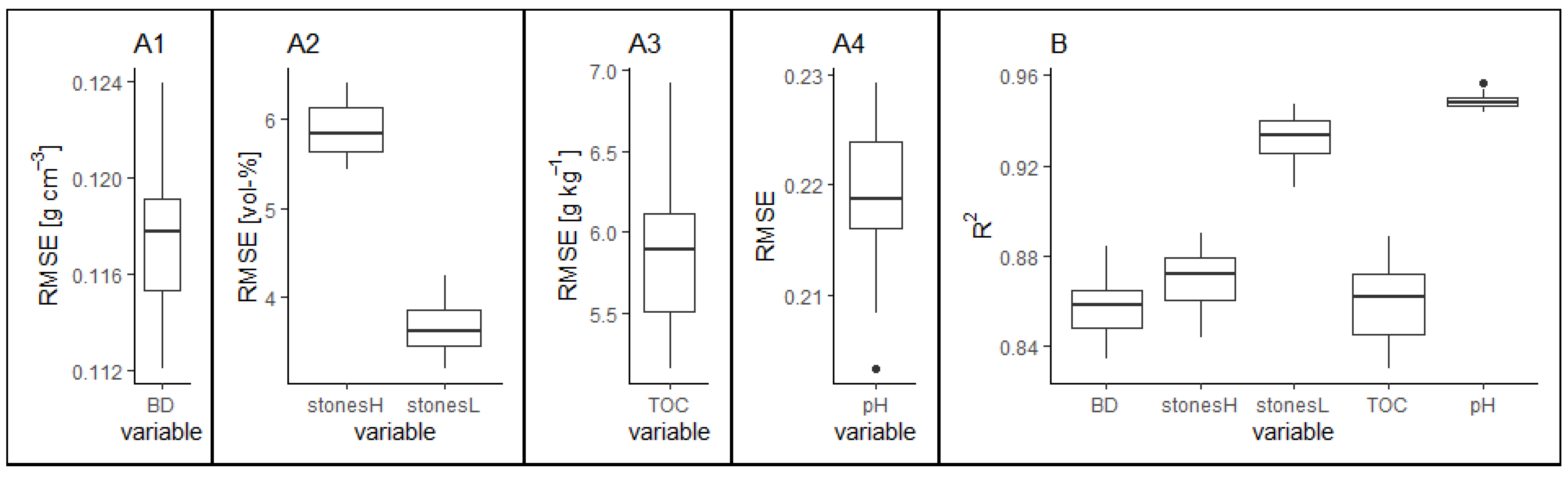
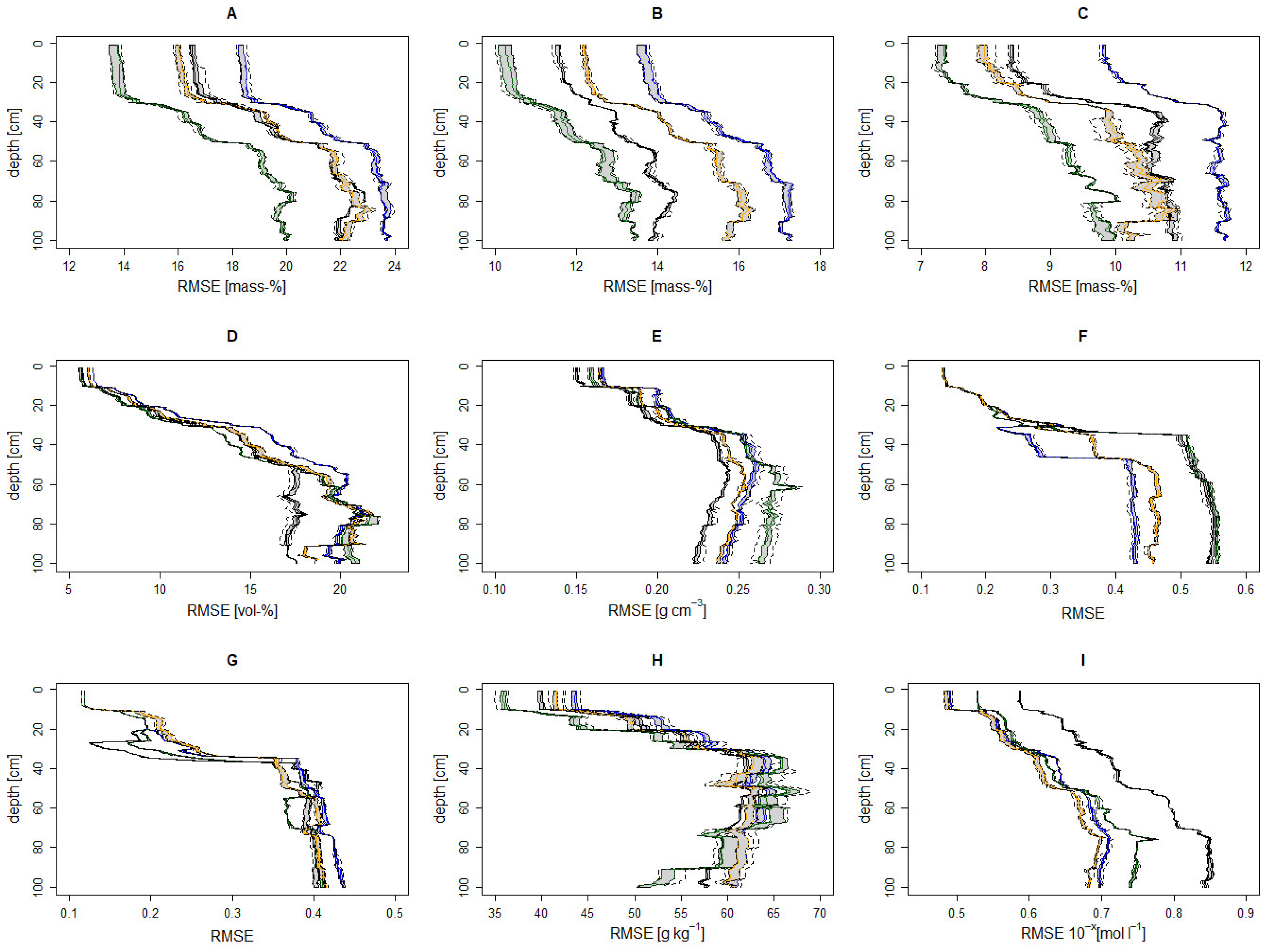
3.3.1. Model Performance

Figure 7 displays the property-wise predictive model performance for the four models RF–PAMp, RF–PAMm, SVM–PAMp, and SVM–PAMm. The performance measure of the approach always depends on two aspects: (1) the statistical dispersion of the multivariate parameter distributions of the SPUs resulting from PAMp or PAMm and (2) the performance of the machine learning algorithm to extract the soil–landscape relation. Consequently, the evaluation of the data product was best achieved in a sense of the predictive RMSE of the individual soil properties.

Regarding soil texture, predictive model performance always detects SVM–PAMp as the best model and RF–PAMm as the least promising, whereas the priority between SVM–PAMm and RF–PAMp favors SVM–PAMm for sand and clay content and RF–PAMp for silt (Figure 7A–C). SVM–PAMp is also the most promising among the four models concerning its predictive performance in terms of the stone content up to a depth of 60 cm (Figure 7D), the prediction of gleyic properties, and the TOC (Figure 7H). Below 60 cm, RF–PAMp shows the best performance for the stone content (Figure 7D). Additionally, this model has the best performance concerning bulk density (Figure 7E). Predicting pH, SVM–PAMm shows the best performance. However, the RMSE of RF–PAMm and SVM–PAMp are only slightly higher. Model performance in reference to stagnic properties is hardly distinguishable between the four models until a depth of 30 cm. This similarity continues for SVM–PAMp and RF–PAMp in the subsoil, while the RMSE of RF–PAMm and SVM–PAMm does not increase as much, resulting in RF–PAMm being the overall best for this property. Altogether, this makes SVM–PAMp the best model for three out of seven soil properties and minor differences for a fourth property.

This indicates the high power of the SVM algorithm when combined with GA optimization for parameter tuning. In contrast, it was expected that RF might result in the overall better algorithm due to its usage in the objective function for SPU optimization. However, the results were ambivalent. RF resulted in the better algorithm for two properties, and SVM for four properties. Overall, this enhances the critical discussion on the common perception that RF is often stated to have the best predictive performance when comparing multiple machine learning algorithms in pedometric modeling applications [63]. The comparison is usually not conducted appropriately since RF does not require much tuning and its most important parameters are natural numbers and, therefore, the common grid-search approach is sufficient. In contrast, the training of SVMs requires thorough tuning of real-valued parameters [4,25]. A fair comparison of the two algorithms is, therefore, only possible if optimization is applied for tuning SVM models.

The overall model performance was decreasing with depth concerning all soil properties, as is commonly perceived in pedometric modeling (e.g.). Figure 7 shows that this decrease was non-linear. For the topsoil, it usually had very good performance, which then rapidly decreased at a certain soil depth. The threshold value differed between the soil properties, though. For the particle size distribution (Figure 7A–C) it ranged around 25 cm, and for the other soil properties, around 10 cm depth (Figure 7D–I). Some of the latter had two steps in the performance decrease, one at 10 cm and another at 25 or 30 cm (bulk density, Figure 7E), 30 or 50 cm (symbol_S, Figure 7F), at 40 cm (symbol_G, Figure 7G), or 25 cm (TOC, Figure 7H) depth. The good topsoil performance with regards to the hydromorphic features was probably due to their onset at a certain soil depth. The other step was likely caused by grassland soils not being separated from cropland soils in the SPU differentiation. This could mean that the difference between grassland soils and cropland soils was minor either with regards to the vertical soil profile differentiation and characteristics or regarding the soil–landscape relation. Concerning the latter, the high number of SCORPAN O predictors from remote sensing data provides a good representation of the land cover and would, therefore, easily allow for this separation between the grassland and cropland soils. With the former, it must be taken into account that the difference between the two only affected a limited number of the considered properties, and then only the respective topsoil. However, this aspect could only be addressed while the calculation of the property-wise profile difference assigned a higher weight to the topsoil differences for these soil properties. The decision on assigning different weights along the depth profile was not trivial, though. A few test runs were conducted with an exponential weight decay function and a step-wise approach. Additionally, optimizing the weights along the depth profile in addition to the already-implemented optimization tasks in PAMp and PAMm would add to the complexity of the objective function and prolong the optimization process to differentiate the SPUs. I would further like to note that the comparison of the RMSE values along the soil profile for certain soil properties can be misleading, as the respective value ranges differed between the various soil depths. This was clearly visible for TOC (Figure 7H), where the predictive model performance seemed to improve at a certain soil depth. However, the lower RMSE values were likely caused by the lower TOC range at this higher soil depth.

In the following, the multivariate 3D data product will be compared to other readily available data products. This is achieved by referring to the predictive median RMSE with regards to the interquartile range of the multivariate parameter distributions along the depth profile. On the one hand, the property- and depth-wise uncertainty will be compared to its first version from Ließ et al. [4]. On the other hand, the national performance estimates (considering agricultural soils) for other spatially continuous data products covering the entirety of Germany were calculated. Table 5 provides an overview. They were evaluated by extracting the predicted property values at the soil survey sites of the test set profile data, which had been used to evaluate the data product developed here. The weighted mean was calculated for the respective depth layer before calculating the RMSE. The compared data products had the following spatial raster resolutions: national scale—100 m [25,64], European scale—500 m [65] and 1000 m [66], and global scale—250 m [67].

Table 5. National-scale evaluation (RMSE) of existing national, European and global-scale data products (considering agricultural soils). The predictive uncertainty was evaluated on behalf of the test set profile data. The values of the raster data products were extracted at the profile sites. A weighted average was calculated for the respective depth interval of the measured data.

Scale of the Data Product	Depth Interval [cm]	Sand Content [Mass-%]	Silt Content [Mass-%]	Clay Content [Mass-%]	Stone Content [Vol-%]	Bulk Density [g cm−3]	TOC [g kg−1]	pH 10−x mol L−1
National	0–30	15.0 [25]	11.8 [25]	8.2 [25]	-	-	22 [64]	-
European	0–20	17.6 [65]	13.8 [65]	9.8 [65]	9 [65]	0.26 [65]	48.3 [66,68]	-
Global [67]	0–5	19.3	16.5	11.4	7.1	0.30	43.6	1.2
	5–15	19.4	16.4	11.0	7.8	0.30	46.2	1.2
	15–30	19.9	17.6	11.7	10.5	0.31	57.6	1.2
	30–60	22.9	18.7	13.8	17.5	0.35	62.4	1.3
	60–100	25.9	19.6	14.3	21.2	0.36	60.7	1.4

Table 5. National-scale evaluation (RMSE) of existing national, European and global-scale data products (considering agricultural soils). The predictive uncertainty was evaluated on behalf of the test set profile data. The values of the raster data products were extracted at the profile sites. A weighted average was calculated for the respective depth interval of the measured data.

Scale of the Data Product	Depth Interval [cm]	Sand Content [Mass-%]	Silt Content [Mass-%]	Clay Content [Mass-%]	Stone Content [Vol-%]	Bulk Density [g cm−3]	TOC [g kg−1]	pH 10−x mol L−1
National	0–30	15.0 [25]	11.8 [25]	8.2 [25]	-	-	22 [64]	-
European	0–20	17.6 [65]	13.8 [65]	9.8 [65]	9 [65]	0.26 [65]	48.3 [66,68]	-
Global [67]	0–5	19.3	16.5	11.4	7.1	0.30	43.6	1.2
	5–15	19.4	16.4	11.0	7.8	0.30	46.2	1.2
	15–30	19.9	17.6	11.7	10.5	0.31	57.6	1.2
	30–60	22.9	18.7	13.8	17.5	0.35	62.4	1.3
	60–100	25.9	19.6	14.3	21.2	0.36	60.7	1.4

With regards to the particle size distribution, the predictive performance improved compared to Ließ et al. [4]. For the sand content, it improved from 14.8 to 13.8 mass-% at 20 cm depth, from 17.5 to 16.3 mass-% at 40 cm depth, and from 20.2 to 19 mass-% at 60 cm depth. Respectively, it improved from 10.7 to 10.4, from 12.2 to 11.6, and from 14.3 to 12.7 mass-% for the silt content, and from 8.2 to 7.5, from 10.1 to 8.9, and from 10.1 to 9.3 mass-% for the clay content. Figure 7A–C show the continuous performance estimates. Concerning the topsoil, the national scale 0–30 cm [25], the European scale 0–20 cm [65], and the global scale 15–30 cm predictions [67] had a higher uncertainty with an RMSE of 15.0, 17.6, and 19.9 mass-% for sand, 11.8, 13.8, and 17.6 mass-% for silt, and 8.2, 9.8, and 11.7 mass-% for clay (Table 5), respectively. For the subsoil, the global scale 30–60 cm predictions [67] also had a higher RMSE. They amounted to 22.9 mass-% for sand, 18.7 mass-% for silt, and 13.8 mass-% for clay (Table 5).

Compared to Ließ et al. [4], the predictive performance concerning the stone content remained more or less the same in the 20 cm depth with 8.1 versus 8.0 vol-%, improved for 40 cm depth from 14.8 to 13.9 vol-%, but was impaired in the 60 cm depth from 16.9 to 19.1 vol-%. For the topsoil, the European (0–20 cm) and global scale (15–30 cm) predictions had a slightly higher uncertainty, with an RMSE of 9 and 10.5 vol-% (Table 5), respectively. Considering the same depth intervals, the RMSE of the data product created here corresponded to an average RMSE of 6.5 vol-% for the 0–20 depth interval and 9.1 vol-% for the 15–30 cm depth interval. This even higher difference in reference to the European data product is due to the overall decrease in uncertainty with lower soil depth (Figure 7D).

For bulk density, the predictive performance was impaired at 20 and 60 cm depths from 0.15 to 0.19, and 0.25 to 0.27 g cm⁻³, but remained the same at the 40 cm depth compared to Ließ et al. [4]. The predictive topsoil uncertainty was still higher for the European and global data products with an RMSE of 0.26 and 0.31 g cm⁻³, respectively. The same applied to the subsoil with an RMSE of 0.35 g cm⁻³ (global predictions 30–60 cm, Table 5).

The predictive model performance along the depth profile with regards to the TOC is displayed in Figure 7H. TOC was not part of the data product generated by Ließ et al. [4]. The averaged RMSE for the respective depth interval was 39.3 compared to 48.3 g kg⁻¹ for Aksoy et al. [66] in the 0–20 cm interval, 43.8 compared to 21 g kg⁻¹ for Sakhaee et al. [64] in the 0–30 cm interval, 38.8 compared to 46.2 g kg⁻¹ in the 5–15 cm, and 49.8 compared to 57. 6 g kg⁻¹ in the 15–30 cm interval for Poggio et al. [67]. This means the data product developed here had a lower predictive topsoil uncertainty compared to the global and European data products, but a higher uncertainty compared to the national data product. One of the reasons for the latter is the high diversity in the soils containing an organic horizon in some part of their profile. The low number of soil profiles representing these soils in the dataset of the agricultural soil inventory had also caused trouble for Sakhaee et al. [64]. They addressed this aspect by training separate models for organic and mineral topsoil, which resulted in an RMSE decrease from 31.6 to 21.0 g kg⁻¹. The complexity increases, though, while multiple properties are jointly considered in 3D. The optimization to differentiate the SPUs merged all these soils into a single SPU (SPU1, Figure 6A1). Compared to the high difference in TOC content between these soils and the all-mineral soils, the TOC differences among the all-mineral soils were minor. Conducting the cluster analysis while applying data transformation to this and other soil properties before calculating the distance matrices did not solve the issue, either. A solution might be to subdivide the data into all-mineral and partly mineral soils and then conduct two separate optimization processes to differentiate the SPUs in each subgroup, as suggested earlier.

The predictive model performance along the depth profile with regards to the pH is displayed in Figure 7I. The pH was not part of the data product generated by Ließ et al. [4]. The averaged RMSE for the respective depth interval was 10^−0.55 compared to 10^−1.2 mol l⁻¹ in the 5–15 cm, and 10^−0.58 compared to 10^−1.2 mol l⁻¹ in the 15–30 cm interval for Poggio et al. [67].

Overall, the models presented here deal with high complexity: They address the multivariate soil variability in 3D compared to the models trained to obtain the univariate 2D data products. It is impressive that a lower predictive uncertainty was still achieved. The lower uncertainty compared to the European and global data products is likely because at national scale for Germany, there are many more data proxies available to approximate the soil-forming factors, namely the expert information contained in the national map products providing information on the soil distribution [41] and parent material [39,40]. This helps in capturing the soil–landscape relation by machine learning. In reference to the national scale data products, a higher performance was achieved for texture, but a lower performance for TOC due to the previously mentioned reasons. Finally, it has to be emphasized that the data product presented here differs from the others. The univariate predictions (single soil property) considered in the comparison provide single-cell predictions for a certain depth interval. In contrast, the data product developed here provides 3D soil information in terms of the multivariate distributions. Its spatial resolution in the 2D mapping space is 100 m, and the resolution along the depth profile is 1 cm. Accordingly, for each raster cell, it provides the slice-wise multivariate distribution of the respective soil properties. It would be inappropriate to consider the median of these distributions for each raster cell. The benefit lies in considering these distributions, which are the consequence of condensing the information contained in the raster cells to a limited number of functional SPUs.

3.3.2. Variable Importance

The VI values (Figure 8) indicate that all predictors were important to a certain extent for all four models. The values are relative, and not comparable between the models.

However, what separates the SVM models (Figure 8C,D) from the RF models (Figure 8A,B) is the high importance they assign to the categorical predictors in comparison to the other predictors. These categorical predictors reflect the inclusion of expert knowledge with regards to parent material and soils included in conventional map products (BAG00, LIT00, STR00, and BGL00) as well as the classified topography (GMK00). Categorical predictors had also proved highly important for the models of the first implementation to represent the agricultural soil landscape of Germany by SPUs [4]. It is unfortunate in this regard that further categorical SCORPAN S and SCORPAN P predictors available at a larger map scale could not be included (e.g. [17,69]). The soil profile database of the agricultural soil inventory does not include sufficient data entries to represent the high number of SMUs included in these maps. The RF models do not prioritize the categorical information, though. This is surprising, as they are known to generally favor categorical predictors [70,71]. In contrast to the latter, they assign comparatively higher importance to the DEM.

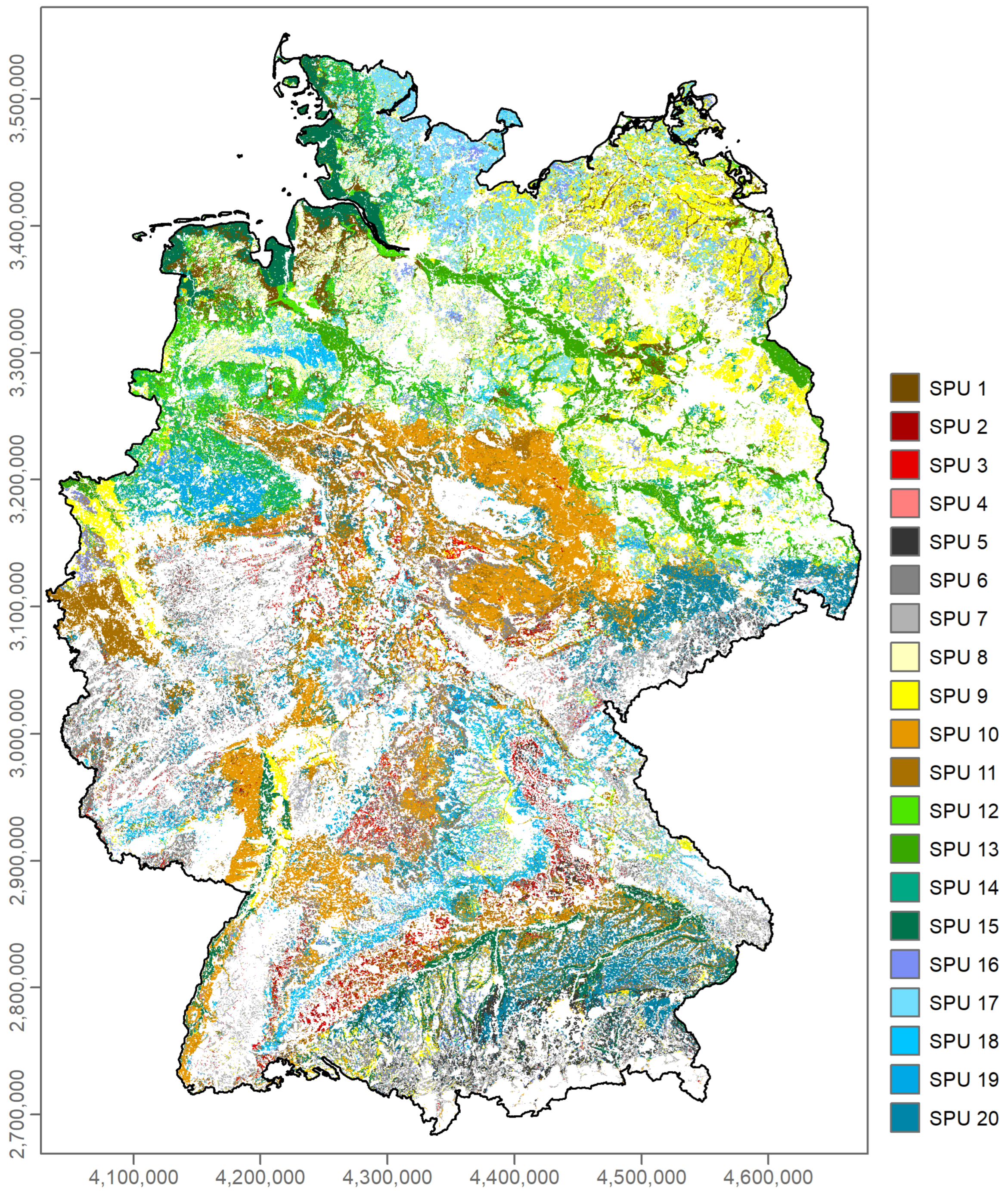
3.3.3. Nationwide Prediction

Figure 9 displays the map of the nationwide prediction of the SPUs with model SVM–PAMp. In the following, it will be described from north to south according to the four morphologic regions of Germany: the North German Lowland, the Central Germany Uplands, the Alpine Foreland, and the Alps.

The North German Lowland presents a mixture of sandy soils (SPU8, SPU 9), stagnic soils (SPU 12–SPU 15) gleyic soils (SPU 16–SPU 19) and patches of the organic SPU 1. Of the sandy soils, SPU 8 dominates in the west, and SPU 9 in the east. SPU 8 has higher sand and correspondingly lower pH values (Figure 6B8,B9,J8,J9). The higher topsoil TOC values of SPU 8 likely originate from the land-use history in this region. Nutrient-poor, sandy topsoil was often improved by mixing it with grass or heather plagues [4]. Stagnic SPU 15 is found along the North Sea coast in the marshland under tidal influence. It is this stagnic SPU that differs from the other stagnic SPUs due to its much lower sand and correspondingly higher silt and clay contents. SPU 14 dominates in the northernmost part, right between the North and Baltic Seas. It is the stagnic SPU whose stagnic properties start at a higher soil depth compared to the others. SPU 12 and SPU 13 are found in the floodplains and lower terraces of the rivers Weser, Elbe, and Oder. The gleyic soils in the north are dominated by SPU 17 along the east coast (Baltic Sea), with patches of this SPU as well as SPU 16, SPU 18, and SPU 19 further inland. SPU 14 and SPU 19 also dominate the area in the southwestern-most part of the North German lowland corresponding to the lowlands of the glacial valleys of the old moraine area [41].

In the Central German Uplands, the Loess plains are represented by SPU 10 and SPU 11. Considering their multivariate distributions, they are mainly differentiated by their pH, with SPU 10 having the higher pH values (Figure 6J10,J11). The gleyic SPU 20 dominates the loess plains in Saxony. It has high silt contents similar to those of SPU 10 and SPU 11. However, large parts of the Central German Uplands are covered by the leptic–skeletic SPUs 2–4 and skeletic SPUs 5–7, which are distinguished by their high stone contents. Of these, SPU 7, with much lower sand contents and correspondingly higher pH values (compared to SPU 5 and SPU 6), dominates. Still, large parts along the Swabian Alp, the Franconian Alp, Spessart, and Franconian Switzerland display high coverage by leptic–skeletic SPU 2, the SPU with the highest depth limitation. The gleyic SPU 18 covers large parts along these mountain ranges. The lower Rhine valley stands out by the domination of sandy SPU 9. Between the cities Karlsruhe and Mainz, SPU 9 is then accompanied by the stagnic SPU 15 with its much lower sand contents. SPU 15 also dominates along the floodplains of the Danube and tributary rivers, which separate the Central German Uplands from the Alpine Foreland. Regarding the considered soil properties, these soils are similar to those along the North Sea coast. To distinguish them from one another, additional soil properties would have to be included. The soils might differ in their electrical conductivity due to the tidal influence along the North Sea coast.

Large parts of the northeast of the Alpine Foreland are covered by the siltic SPU 10 as well as the gleyic SPU 20, having a similar texture. This indicates the similarity of these soils to the Loess plains. Additionally, they co-occur with gleyic SPU 16, which has higher sand contents. Large parts of the remaining region are dominated by the leptic–skeletic SPU 2 and SPU 4, while patches of the sandy SPU 9 and organic SPU 1 are also clearly distinguishable. Large parts of the Alps are not under agricultural use. Those that are often contain high stone contents (SPU 3, SPU 5, and SPU 6) and are partly limited in depth (SPU 3). Still, the sandy SPU 9, silty SPU 10, stagnic SPU 15, and gleyic SPU 16 also occur.

Overall the number of SPUs increased from 8 to 20 in comparison to Ließ et al. [4], providing a more detailed spatial differentiation. The previous single SPU with a high stone content and a depth limitation in the top 100 cm is now augmented to six SPUs with a high stone content, of which three additionally have a depth limitation in their top 100 cm. The two SPUs with stagnic and two with gleyic properties were augmented to four and five, respectively. The SPUs with a predominantly sandy or silty texture were augmented from one SPU to two SPUs in both cases. Simply, the SPU including soils with organic horizons remained only one, another hint to consider the separate differentiation into SPUs for the all-mineral and partly mineral soils.

The pattern of the spatial allocation of the SPUs shows some similarity with regards to the national-scale soil map products BÜK200 and BÜK1000 [17,72]. This was expected considering the high importance of the SCORPAN P, SCORPAN R, and SCORPAN S predictors. Ultimately, the national soil maps also heavily rely on topography and parent material. As mentioned previously, the information contained in the spatial units differs. Complex SMUs composed of multiple co-occurring soils differing largely in their profile characteristics are by no means comparable to spatially allocated SPUs, each being described by a multivariate parameter distribution along the depth profile. It is interesting to note, though, that the data product provided here is a national-scale representation with much fewer SPUs than the SMUs in these soil maps.

4. Conclusions

The national-scale evaluation and modeling of the impact of agricultural management and climate change on soils, crop growth, and the environment require soil information at a spatial resolution addressing individual agricultural fields. The agglomeration of the soil parameter space into a limited number of functional SPUs allows for reducing the required resources to run agricultural process models without having to cut back on the spatial resolution. To serve these needs, creative data science approaches are needed.

Here, two data science approaches were developed involving unsupervised classification to generate a multivariate 3D data product of spatially allocated functional SPUs, each being defined by a multivariate parameter distribution along the depth profile from 0 to 100 cm. The two methods account for differences in variable types and distributions and involve genetic algorithm optimization to identify those SPUs with the lowest internal variability and maximum inter-unit difference with regards to both their soil characteristics and landscape setting.

The high potential of these two approaches was demonstrated by applying them to the agricultural German soil landscape. The resulting data product consists of 20 SPUs that are each described by a multivariate parameter distribution along the depth profile from 0 to 100 cm. It comes along with property- and depth-wise uncertainty estimates. Its spatial resolution in the 2D mapping space is 100 m, and the resolution along the depth profile is 1 cm. It is available in a reduced storage format consisting of two related files, (1) a nationwide raster file with identifiers pointing to (2) the respective multivariate distribution for each functional SPU provided in table format. Each property’s distribution is represented by the 5, 25, 50, 75 and 95% quantiles.

The spatial pattern of the nationwide raster shows some similarity with the national soil maps of Germany. The information contained in the spatial units differs, though. Complex SMUs composed of multiple co-occurring SUs of very different characteristics are by no means comparable to spatially allocated SPUs that are each represented by a multivariate parameter distribution. Furthermore, it is interesting that the data product created here is a national-scale representation with significantly fewer SPUs than the SMUs in these soil maps. Additionally, the boundaries of the SPUs differ from those of the SMUs. Why the boundaries differ and whether the number of SPUs would increase if a larger soil profile database is included are two aspects that are valuable to investigate together with colleagues from the soil survey institutes.

The created data product is the second version of such a 3D soil-landscape model for the agricultural landscape of Germany. Compared to Version 1, the number of SPUs increased, and the respective interquartile range of the multivariate distributions and the predictive uncertainty were reduced. Additionally, two further soil properties, TOC and pH, were included. Version 2 of the data product also has a lower uncertainty compared to existing univariate 2D data products while considering the interquartile range of the multivariate distributions. I recommend using them as margins to run agricultural process models. Limitations concerning TOC uncertainty suggest considering all-mineral and partly mineral soils separately in the SPU differentiation. Whether the available data are sufficient to follow such an approach would have to be tested, though.

References

1. Kapoor, D.; Bhardwaj, S.; Landi, M.; Sharma, A.; Ramakrishnan, M.; Sharma, A. The Impact of Drought in Plant Metabolism: How to Exploit Tolerance Mechanisms to Increase Crop Production. Appl. Sci. 2020, 10, 5692. [Google Scholar] [CrossRef]
2. Magombeyi, M.S.; Taigbenu, A.E.; Barron, J. Effectiveness of Agricultural Water Management Technologies on Rainfed Cereals Crop Yield and Runoff in Semi-Arid Catchment: A Meta-Analysis. Int. J. Agric. Sustain. 2018, 16, 418–441. [Google Scholar] [CrossRef]
3. Hatfield, J.L.; Dold, C. Water-Use Efficiency: Advances and Challenges in a Changing Climate. Front. Plant Sci. 2019, 10, 103. [Google Scholar] [CrossRef] [PubMed] [Green Version]
4. Ließ, M.; Gebauer, A.; Don, A. Machine Learning With GA Optimization to Model the Agricultural Soil-Landscape of Germany: An Approach Involving Soil Functional Types With Their Multivariate Parameter Distributions Along the Depth Profile. Front. Environ. Sci. 2021, 9, 212. [Google Scholar] [CrossRef]
5. Searle, R.; McBratney, A.; Grundy, M.; Kidd, D.; Malone, B.; Arrouays, D.; Stockman, U.; Zund, P.; Wilson, P.; Wilford, J.; et al. Digital Soil Mapping and Assessment for Australia and beyond: A Propitious Future. Geoderma Reg. 2021, 24, e00359. [Google Scholar] [CrossRef]
6. Mueller, L.; Schindler, U.; Mirschel, W.; Graham Shepherd, T.; Ball, B.C.; Helming, K.; Rogasik, J.; Eulenstein, F.; Wiggering, H. Assessing the Productivity Function of Soils. A Review. Agron. Sustain. Dev. 2010, 30, 601–614. [Google Scholar] [CrossRef]
7. Wallach, D.; Palosuo, T.; Thorburn, P.; Mielenz, H.; Buis, S.; Hochman, Z.; Gourdain, E.; Garcia, C.; Andrianasolo, F.; Dumont, B.; et al. Calibration of Crop Phenology Models: Going beyond Recommendations. bioRxiv 2022. [Google Scholar] [CrossRef]
8. Boeing, F.; Rakovech, O.; Kumar, R.; Samaniego, L.; Schrön, M.; Hildebrandt, A.; Rebmann, C.; Thober, S.; Müller, S.; Zacharias, S.; et al. High-Resolution Drought Simulations and Comparison to Soil Moisture Observations in Germany. Hydrol. Earth Syst. Sci. 2022, 26, 5137–5161. [Google Scholar] [CrossRef]
9. Bönecke, E.; Breitsameter, L.; Brüggemann, N.; Chen, T.W.; Feike, T.; Kage, H.; Kersebaum, K.C.; Piepho, H.P.; Stützel, H. Decoupling of Impact Factors Reveals the Response of German Winter Wheat Yields to Climatic Changes. Glob. Chang. Biol. 2020, 26, 3601–3626. [Google Scholar] [CrossRef]
10. Webber, H.; Lischeid, G.; Sommer, M.; Finger, R.; Nendel, C.; Gaiser, T.; Ewert, F. No Perfect Storm for Crop Yield Failure in Germany. Environ. Res. Lett. 2020, 15, 104012. [Google Scholar] [CrossRef]
11. Drastig, K.; Prochnow, A.; Libra, J.; Koch, H.; Rolinski, S. Irrigation Water Demand of Selected Agricultural Crops in Germany between 1902 and 2010. Sci. Total Environ. 2016, 569–570, 1299–1314. [Google Scholar] [CrossRef] [PubMed]
12. Chen, S.; Arrouays, D.; Angers, D.A.; Chenu, C.; Barré, P.; Martin, M.P.; Saby, N.P.A.; Walter, C. National Estimation of Soil Organic Carbon Storage Potential for Arable Soils: A Data-Driven Approach Coupled with Carbon-Landscape Zones. Sci. Total Environ. 2019, 666, 355–367. [Google Scholar] [CrossRef] [PubMed]
13. Wiesmeier, M.; von Lützow, M.; Wollschlaeger, U.; Vogel, H.J.; Garcia-Franco, N.; Ließ, M.; Urbanski, L.; Hobley, E.; Lang, B.; Marin-Spiotta, E.; et al. Soil Organic Carbon Storage as a Key Function of Soils—A Review of Drivers and Indicators at Various Scales. Geoderma 2019, 333, 149–162. [Google Scholar] [CrossRef]
14. Wang, C.; Amon, B.; Schulz, K.; Mehdi, B. Factors That Influence Nitrous Oxide Emissions from Agricultural Soils as Well as Their Representation in Simulation Models: A Review. Agronomy 2021, 11, 770. [Google Scholar] [CrossRef]
15. Bouraoui, F.; Grizzetti, B. Modelling Mitigation Options to Reduce Diffuse Nitrogen Water Pollution from Agriculture. Sci. Total Environ. 2014, 468–469, 1267–1277. [Google Scholar] [CrossRef]
16. Sundermann, G.; Wägner, N.; Cullmann, A.; von Hirschhausen, C.R.; Kemfert, C. Nitrate Pollution of Groundwater Long Exceeding Trigger Value: Fertilization Practices Require More Transparency and Oversight, DIW Weekly Report; DIW Weekly; Deutsches Institut für Wirtschaftsforschung (DIW): Berlin, Germany, 2020. [Google Scholar]
17. BGR. Soil Map of Germany 1:250,000; Federal Institute for Geosciences and Natural Resources: Hanover, Germany, 2018.
18. Ad-hoc-AG Boden. Bodenkundliche Kartieranleitung. KA5, 5th ed.; Bundesanstalt für Geowissenschaften und Rohstoffe in Zusammenarbeit mit den Staatlichen Geologischen Diensten: Stuttgart, Germany, 2005; ISBN 978-3-510-95920-4.
19. Jenny, H. Factors of Soil Formation. A System of Quantitative Pedology; Dover Publications: New York, NY, USA, 1941. [Google Scholar]
20. McBratney, A.B.; Mendonca Santos, M.L.; Minasny, B. On Digital Soil Mapping. Geoderma 2003, 117, 352. [Google Scholar] [CrossRef]
21. Padarian, J.; Minasny, B.; McBratney, A.B. Machine Learning and Soil Sciences: A Review Aided by Machine Learning Tools. Soil 2020, 6, 35–52. [Google Scholar] [CrossRef] [Green Version]
22. Arrouays, D.; Mulder, V.L.; Richer-de-Forges, A.C. Soil Mapping, Digital Soil Mapping and Soil Monitoring over Large Areas and the Dimensions of Soil Security—A Review. Soil Secur. 2021, 5, 100018. [Google Scholar] [CrossRef]
23. Chen, S.; Arrouays, D.; Leatitia Mulder, V.; Poggio, L.; Minasny, B.; Roudier, P.; Libohova, Z.; Lagacherie, P.; Shi, Z.; Hannam, J.; et al. Digital Mapping of GlobalSoilMap Soil Properties at a Broad Scale: A Review. Geoderma 2022, 409, 115567. [Google Scholar] [CrossRef]
24. Daniel, Ž.; Minařík, R.; Skála, J.; Beitlerová, H.; Juřicová, A.; Rojas, J.R.; Penížek, V.; Zádorová, T. High-Resolution Agriculture Soil Property Maps from Digital Soil Mapping Methods, Czech Republic. Catena 2022, 212, 106024. [Google Scholar] [CrossRef]
25. Gebauer, A.; Sakhaee, A.; Don, A.; Poggio, M.; Ließ, M. Topsoil Texture Regionalization for Agricultural Soils in Germany—An Iterative Approach to Advance Model Interpretation. Front. Soil Sci. 2022, 1, 25. [Google Scholar] [CrossRef]
26. Malone, B.; Searle, R. Updating the Australian Digital Soil Texture Mapping (Part 2): Spatial Modelling of Merged Field and Lab Measurements. Soil Res. 2021, 59, 419–434. [Google Scholar] [CrossRef]
27. Reddy, N.N.; Chakraborty, P.; Roy, S.; Singh, K.; Minasny, B.; McBratney, A.B.; Biswas, A.; Das, B.S. Legacy Data-Based National-Scale Digital Mapping of Key Soil Properties in India. Geoderma 2021, 381, 114684. [Google Scholar] [CrossRef]
28. Padarian, J.; Minasny, B.; McBratney, A.B. Using Deep Learning for Digital Soil Mapping. Soil 2019, 5, 79–89. [Google Scholar] [CrossRef] [Green Version]
29. Ma, Y.; Minasny, B.; McBratney, A.; Poggio, L.; Fajardo, M. Predicting Soil Properties in 3D: Should Depth Be a Covariate? Geoderma 2021, 383, 114794. [Google Scholar] [CrossRef]
30. Poeplau, C.; Don, A.; Flessa, H.; Heidkamp, A.; Jacobs, A.; Prietz, R. First German Agricultural Soil Inventory–Core Dataset; Open Agrar Repositorium: Göttingen, Germany, 2020. [Google Scholar] [CrossRef]
31. Jacobs, A.; Flessa, H.; Don, A.; Heidkamp, A.; Prietz, R.; Gensior, A.; Poeplau, C.; Riggers, C.; Tiemeyer, B.; Vos, C.; et al. Landwirtschaftlich Genutzte Böden in Deutschland–Ergebnisse Der Bodenzustandserhebung, Thünen Report 64; Johann Heinrich von Thünen-Institut: Braunschweig, Germany, 2018; ISBN 9783865761927. [Google Scholar]
32. DWD. Seasonal Grids of Sum of Precipitation over Germany, Version v1.0. Available online: https://opendata.dwd.de/climate_environment/CDC/grids_germany/seasonal/precipitation/ (accessed on 23 October 2022).
33. DWD. Seasonal Grids of Monthly Averaged Daily Air Temperature (2m) over Germany, Version v1.0. Available online: https://opendata.dwd.de/climate_environment/CDC/grids_germany/seasonal/air_temperature_mean/ (accessed on 23 October 2022).
34. DWD. Seasonal Grids of Sum of Drought Index (de Martonne) over Germany, Version v1.0. Available online: https://opendata.dwd.de/climate_environment/CDC/grids_germany/seasonal/drought_index/ (accessed on 23 October 2022).
35. Swinnen, E.; Van Hoolst, R. Copernicus Global Land Operations ”Vegetation and Energy”. Issue I1.12, Version 1. Available online: https://land.copernicus.eu/global/sites/cgls.vito.be/files/products/CGLOPS1_ATBD_DMP300m-V1_I1.12.pdf (accessed on 23 October 2022).
36. Swinnen, E.; Dierckx, W.; Toté, C. Gio Global Land Component–Lot I ”Operation of the Global Land Component”. Quality Assessment Report Proba-V NDVI, VCI and VPI. Issue 1.21. Available online: https://land.copernicus.eu/global/sites/cgls.vito.be/files/products/GIOGL1_QAR_NDVI-VCI-VPI_I1.21.pdf (accessed on 23 October 2022).
37. BGR. Geomorphographic Map of Germany, GMK1000; Federal Institute for Geosciences and Natural Resources: Hanover, Germany, 2007.
38. European Environment Agency (EEA). Copernicus Land Monitoring Service—EU-DEM, European Digital Elevation Model Version 1.1.; EEA: Copenhagen, Denmark, 2017.
39. BGR; SDG. Hydrogeological Map of Germany 1:250,000 (HÜK250); Federal Institute for Geosciences and Natural Resources (BGR): Hanover, Germany; German State Geological Surveys (SGD): Hanover, Germany, 2019.
40. BGR. Groups of Soil Parent Material in Germany 1:5,000,000. BAG5000, Version 3.0; Federal Institute for Geosciences and Natural Resources: Hanover, Germany, 2008.
41. BGR. Soil Scapes in Germany 1:5,000,000. BGL5000; Federal Institute for Geosciences and Natural Resources: Hanover, Germany, 2008.
42. INSPIRE Thematic Working Group. INSPIRE–Infrastructure for Spatial Information in Europe. D2.8.I.2 Data Specification on Geographical Grid Systems–Technical Guidelines; INSPIRE Thematic Working Group Coordinate Reference Systems & Geographical Grid Systems: Brussels, Belgium, 2014. [Google Scholar]
43. Conrad, O.; Bechtel, B.; Bock, M.; Dietrich, H.; Fischer, E.; Gerlitz, L.; Wehberg, J.; Wichmann, V.; Böhner, J. System for Automated Geoscientific Analyses (SAGA) v. 2.1.4. Geosci. Model Dev. 2015, 8, 1991–2007. [Google Scholar] [CrossRef] [Green Version]
44. Kaufman, L.; Rousseeuw, P.J. Finding Groups in Data: An Introduction to Cluster Analysis; John Wiley & Sons, Inc.: Hoboken, NJ, USA, 1990; ISBN 9780471878766. [Google Scholar]
45. Ahmad, A.; Khan, S.S. Survey of State-of-the-Art Mixed Data Clustering Algorithms. IEEE Access 2019, 7, 31883–31902. [Google Scholar] [CrossRef]
46. Van Mechelen, I.; Boulesteix, A.-L.; Dangl, R.; Dean, N.; Guyon, I.; Hennig, C.; Leisch, F.; Steinley, D. Benchmarking in Cluster Analysis: A White Paper. arXiv 2018, arXiv:1809.10496. [Google Scholar]
47. Rousseeuw, P.J. Silhouettes: A Graphical Aid to the Interpretation and Validation of Cluster Analysis. J. Comput. Appl. Math. 1987, 20, 53–65. [Google Scholar] [CrossRef] [Green Version]
48. Breiman, L. Random Forests. J. Chem. Inf. Model. 2001, 53, 1689–1699. [Google Scholar] [CrossRef]
49. Ishwaran, H.; Kogalur, U.B. Package ‘RandomForestSRC’. Fast Unified Random Forests for Survival, Regression, and Classification (RF-SRC). Version 3.1.1. 2022. Available online: https://www.randomforestsrc.org/ (accessed on 23 October 2022).
50. Hothorn, T.; Hornik, K.; Strobl, C.; Zeileis, A. Package ‘Party’. A Laboratory for Recursive Partytioning. Version 1.3-11. 2022. Available online: http://party.r-forge.r-project.org/ (accessed on 23 October 2022).
51. Cortes, C.; Vapnik, V. Support-Vector Networks. Mach. Leaming 1995, 20, 273–297. [Google Scholar] [CrossRef]
52. Chang, C.-C.; Lin, C.-J. LIBSVM: A Library for Support Vector Machines. ACM Trans. Intell. Syst. Technol. 2011, 2, 1–39. [Google Scholar] [CrossRef]
53. Meyer, D. Support Vector Machines—The Interface to Libsvm in Package E1071. FH Tech. Wien 2019, 16, 130. [Google Scholar]
54. Hastie, T.; Tibshirani, R.; Friedman, J. The Elements of Statistical Learning–Data Mining, Inference, and Prediction, 2nd ed.; Springer Science+Business Media, LLC: New York, NY, USA, 2009; ISBN 978-0-387-84857-0. [Google Scholar]
55. Affenzeller, M.; Winkler, S.; Wagner, S.; Beham, A. Genetic Algorithms and Genetic Programming; Taylor and Francis Group: Boca Raton, FL, USA, 2009; ISBN 978-1-58488-629-7. [Google Scholar]
56. Batjes, N. A Taxotransfer Rule Based Approach for Filling Gaps in Measured Soil Data in Primary SOTER Databases (Version 1.1); World Soil Information: Wageningen, The Netherlands, 2003. [Google Scholar]
57. Hugelius, G.; Bockheim, J.G.; Camill, P.; Elberling, B.; Grosse, G.; Harden, J.W.; Johnson, K.; Jorgenson, T.; Koven, C.D.; Kuhry, P.; et al. A New Data Set for Estimating Organic Carbon Storage to 3 m Depth in Soils of the Northern Circumpolar Permafrost Region. Earth Syst. Sci. Data 2013, 5, 393–402. [Google Scholar] [CrossRef] [Green Version]
58. Almendra-Martín, L.; Martínez-Fernández, J.; Piles, M.; González-Zamora, Á. Comparison of Gap-Filling Techniques Applied to the CCI Soil Moisture Database in Southern Europe. Remote Sens. Environ. 2021, 258, 112377. [Google Scholar] [CrossRef]
59. Wang, Q.; Wang, L.; Zhu, X.; Ge, Y.; Tong, X.; Atkinson, P.M. Remote Sensing Image Gap Filling Based on Spatial-Spectral Random Forests. Sci. Remote Sens. 2022, 5, 100048. [Google Scholar] [CrossRef]
60. Taki, R.; Wagner-Riddle, C.; Parkin, G.; Gordon, R.; VanderZaag, A. Comparison of Two Gap-Filling Techniques for Nitrous Oxide Fluxes from Agricultural Soil. Can. J. Soil Sci. 2019, 99, 12–24. [Google Scholar] [CrossRef]
61. Kim, Y.; Johnson, M.S.; Knox, S.H.; Black, T.A.; Dalmagro, H.J.; Kang, M.; Kim, J.; Baldocchi, D. Gap-Filling Approaches for Eddy Covariance Methane Fluxes: A Comparison of Three Machine Learning Algorithm Algorithms and Algorithm a Traditional Method with Principal Component Analysis. Glob. Chang. Biol. 2020, 26, 1499–1518. [Google Scholar] [CrossRef]
62. Ghanbarian, B.; Pachepsky, Y. Machine Learning in Vadose Zone Hydrology: A Flashback. Vadose Zo. J. 2022, 21, e20212. [Google Scholar] [CrossRef]
63. Lamichhane, S.; Kumar, L.; Wilson, B. Digital Soil Mapping Algorithms and Covariates for Soil Organic Carbon Mapping and Their Implications: A Review. Geoderma 2019, 352, 395–413. [Google Scholar] [CrossRef]
64. Sakhaee, A.; Gebauer, A.; Ließ, M.; Don, A. Spatial Prediction of Organic Carbon in German Agricultural Topsoil Using Machine Learning Algorithms. Soil 2022, 8, 587–604. [Google Scholar] [CrossRef]
65. Ballabio, C.; Panagos, P.; Monatanarella, L. Mapping Topsoil Physical Properties at European Scale Using the LUCAS Database. Geoderma 2016, 261, 110–123. [Google Scholar] [CrossRef]
66. Aksoy, E.; Yigini, Y.; Montanarella, L. Combining Soil Databases for Topsoil Organic Carbon Mapping in Europe. PLoS ONE 2016, 11, 2022. [Google Scholar] [CrossRef] [PubMed]
67. Poggio, L.; De Sousa, L.M.; Batjes, N.H.; Heuvelink, G.B.M.; Kempen, B.; Ribeiro, E.; Rossiter, D. SoilGrids 2.0: Producing Soil Information for the Globe with Quantified Spatial Uncertainty. Soil 2021, 7, 217–240. [Google Scholar] [CrossRef]
68. Van Liedekerke, M.; Panagos, P. Predicted Distribution of SOC Content in Europe (Based on LUCAS, BioSoil and CZO) in the Context of the EU-Funded SoilTrEC Project. PLoS ONE 2016, 11, e0152098. [Google Scholar]
69. BGR. General Geological Map of the Federal Republic of Germany 1:200,000; Federal Institute for Geosciences and Natural Resources: Hanover, Germany, 2007.
70. Probst, P.; Wright, M.N.; Boulesteix, A.L. Hyperparameters and Tuning Strategies for Random Forest. Wiley Interdiscip. Rev. Data Min. Knowl. Discov. 2019, 9, e1301. [Google Scholar] [CrossRef] [Green Version]
71. Strobl, C.; Boulesteix, A.-L.; Zeileis, A.; Hothorn, T. Bias in Random Forest Variable Importance Measures: Illustrations, Sources and a Solution. BMC Bioinformatics 2007, 8, 25. [Google Scholar] [CrossRef]
72. BGR. Soil Map of Germany 1:1,000,000. BÜK1000; Federal Institute for Geosciences and Natural Resources: Hanover, Germany, 2013.
Figure 1. Objective function of the optimization process for SPU differentiation with PAMp. All white boxes are required input data. White ovals reflect parameters that are optimized. Pw = vector of P weights, dist = distance matrix, ndist = normalized distance matrix, nSPdist = normalized single-property distance matrices, nclus = number of clusters, PAM = partitioning around medoids clustering, Pdata = predictor data, Rdata = response data, PRdata = predictor-response data, RF = random forest.
Agriculture 12 01784 g001
Figure 2. Multistep clustering part of the objective function of the optimization process for SPU differentiation with PAMm. All white boxes are required input data. White ovals reflect parameters that are optimized. ndist = normalized distance matrix, nclu = maximum number of clusters to test in each step, sil = threshold of the Silhouette Index, silmin minimum Silhouette Index value, pmin minimum number of profiles in each cluster, nd = normalized distance matrix subset, PAM = partitioning around medoids clustering, Rdata = response data, nclus number of clusters.
Agriculture 12 01784 g002
Figure 3. Predictive model performance of the RF models for gap filling. (A) RMSE boxplots of 25 models, (B) R2 boxplots of 25 models. BD = bulk density, stonesF = stone content from dataF, stonesL = stone content from dataL, and TOC = total organic carbon content.
Agriculture 12 01784 g003
Figure 4. Relative variable importance values (VI) of the RF models for gap filling. (A) Bulk density, (B) stonesF (stone content from dataF), (C) stonesL (stone content from dataL), (D) TOC, and (E) pH. P_ * = value corresponding to the whole profile (* stands for any following variable indicator). H_ * = property values of the horizon to be gap-filled. Ha_ * property values of the overlying horizon, Hb_ * property values of the underlying horizon, H1 = value of the uppermost horizon, Hl = value of the last horizon, porg = percentage of organic horizons, thick = thickness, mat = horizon material (mineral, organic, bedrock).
Agriculture 12 01784 g004
Figure 5. PAMm subdivision tree of the step-wise procedure. The light grey color indicates that the cluster obtained by the respective step is already a final cluster, which will not be further subdivided in the subsequent clustering steps.
Agriculture 12 01784 g005
Figure 6. Multivariate soil parameter distributions along the depth profile of the SPUs obtained with PAMp. The figure columns reflect the respective SPUs 1 to 20, figure lines refer to the various soil properties. (A) The slice-wise contribution of profiles with mineral properties (dark grey), organic properties (black) or bedrock (light-grey). The white numbers indicate the number of profiles supporting the respective SPU. (B) Sand content, (C) silt content, (D) clay content, (E) stone content, (F) bulk density, (G) symbol_S, (H) symbol_G, (I) TOC, and (J) pH. In figure (B) to (J), the solid line indicates the median of the distribution, the shaded area between dotted lines reflects the interquartile range, the other dotted line reflects the 5% quantile, and the dashed line reflects the 95% quantile. Please be aware that figures (I) have different X-axis ranges, namely (I1) = 0–600, (I12) to (I15) = 0–200, and all others = 0–100.
Agriculture 12 01784 g006aAgriculture 12 01784 g006b
Figure 7. Predictive model performance considering the interquartile range of the SPUs’ multivariate distribution along the depth profile. (A) sand content, (B) silt content, (C) clay content, (D) stone content, (E) bulk density, (F) symbol_S, (G) symbol_G, (H) TOC, and (I) pH. The colors reflect the different models: black = RF−PAMp, blue = RF−PAMm, green = SVM−PAMp, yellow = SVM−PAMm. The lines along the shaded area correspond to the lower and upper hinges of the five predicted values (repeated CV), the solid line to the median, and the dotted lines to the upper and lower whiskers.
Agriculture 12 01784 g007
Figure 8. Variable importance (VI) boxplots of the models for SPU regionalization. (A) RF–PAMp, (B) RF–PAMm, (C) SVM–PAMp, and (D) SVM–PAMm. The horizontal lines separate the respective predictor groups corresponding to the SCORPAN factors: climate, organisms, relief (topography), relief (hydrology), relief (categorical), parent material, soil, and latitude and longitude. Please refer to Table 1 for the predictor abbreviations.
Agriculture 12 01784 g008
Figure 9. Map of Germany displaying the distribution of the SPUs corresponding to model SVM–PAMp. Colors were selected to emphasize the groups: SPU 1 organic, SPU 2—SPU 4 leptic–skeletic, SPU 5—SPU 7 skeletic, SPU 8—SPU 9 sandy, SPU 10—SPU 11 silty, SPU 12—SPU 15 stagnic, and SPU 16—SPU 20 gleyic SPUs. Non-agricultural areas are masked. Coordinate reference system EPSG 3035.
Agriculture 12 01784 g009