Influencing the Success of Precision Farming Technology Adoption—A Model-Based Investigation of Economic Success Factors in Small-Scale Agriculture

Abstract

Even more than 30 years after the introduction of precision farming technologies and studies of their benefits in terms of productivity gains and environmental improvements, adoption rates, especially for variable-rate technologies, are very low. In particular, in smallholder areas, farm managers are reluctant to adopt these technologies. Therefore, this study identifies factors that hinder or facilitate adoption from an economic perspective. Using a model-based sensitivity analysis with three farms of different sizes (11 ha, 57 ha and 303 ha), it is shown that larger farms have higher resilience to external factors due to economies of scale. In addition, it is clarified that the certainty of obtaining additional benefits with GPS guidance systems can explain the higher adoption rates in farming practice, although the additional benefits (per hectare and year) are much lower for this technology than for variable-rate technologies. Small farms (>30 ha) are by no means excluded from the use of digital technologies, as it is shown that the influence of learning costs on profitability is very low, low subsidies can lead to a drastic reduction in the minimum farm size and the presence of low-cost technologies is an efficient solution which allows small farms to participate in the digital transformation of agriculture.

1. Introduction

Agriculture is constantly facing new challenges. The demands for more efficient land management originate, among other factors, from population growth, land sealing and the expected shortage of fossil fuel [1,2,3,4]. Numerous studies have shown that technological progress offers possible solutions for the sustainable intensification of agriculture [5,6,7]. Precision farming technologies, as they have been known since the late 1990s, on the one hand, take advantage of a global positioning system (GPS) for more precise management in order to bring about savings in inputs without sacrificing yields [8,9,10]. On the other hand, it is possible to react to differences in growing conditions, and, for example, to increase yields and qualities, by redistributing the amount of fertilizer that has been applied uniformly [9,10,11]. The global positioning system has its origins in military use, but its field of application has expanded beyond that into the civilian sector, for example, in the navigation of vehicles, the determination of exact geographical positions and the use in the agricultural sector mentioned above [12].

Conversely, numerous studies have shown that, although these technologies have been available for more than 30 years as a solution to the above-mentioned problems, adoption rates in agricultural practice are very low, especially in small-structured areas [13,14,15,16]. The current study in the small-structured state of Bavaria shows that less than 5% of the farmers surveyed use site-specific fertilization technology [17]. Similar data can be found in the study by Groher et al. in small-structured Switzerland, which assumed an adoption rate of 17% for electronic measuring systems (e.g., N sensor) [18]. Since, in this study, site-specific fertilization is only one technology out of a total of seven in this group, a much lower adoption rate than 17% can be assumed. Thus, there appears to be a gap between actual adoption rates in practice and the perceptions of manufacturers, scientists and policymakers [15].

The reasons for this can be manifold and have, so far, mostly been approached from a socioeconomic perspective with consideration of the general reasons for technology acceptance, without mentioning specific economic measures [8,19,20]. Kernecker et al. [21], for example, assumed that the multitude of possibilities and the complexity of the technologies can lead to a hesitant attitude on the part of farmers. Other authors emphasized the scale dependency of technology use due to the still relatively high investment costs, which make it difficult for small farms in particular to enter digital farming [8,22,23,24,25]. A few authors addressed the problem of difficult-to-estimate learning costs or implementation effort, but they did not provide a specific assessment of the extent to which implementation effort affects the economical use of digital technologies [13,19,26,27,28].

In addition, no economic evaluations of implementation at the farm level that provide a complete view of the changes in the farm are known to date. At the crop level, only individual technology variants have been studied, which does not allow any general conclusions to be drawn about system changes and success factors [29,30,31]. Other authors mentioned the uncertainty on the matter of additional benefits and, therefore, mainly examined the cost structure of precision farming technologies [25,32]. In any case, small farms are often excluded by the selection of data in different studies (examined farms between 300–2000 ha) [26,33].

The demand from science for the use of existing technological possibilities is made clear by Finger et al. [34], who suggested that a broader application should be forced due to the economic and environmental advantages of precision farming technologies. This is complemented by voices from politics, which, using the example of the “Farm to Fork Strategy” (presented by the European Commission), demand, e.g., savings in inputs (fertilizer/crop protection) and, thus, indirectly point to the necessity of using precision farming technologies, among other things [35].

Consequently, there is a gap between the desired diffusion of digital technologies, actual adoption rates in farming practices and the potential benefits of these technologies for more sustainable smallholder agriculture. Since previous research has not explicitly addressed these issues, this study aims to close this gap by identifying where barriers exist and where facilitating factors should be sought from an economic perspective.

Using the example of a smallholder farming region in Germany (Baden-Wuerttemberg) and two different technology groups (yield-enhancing and input-saving technologies), this study investigates (i) which factors relating to revenue, direct cost and variable and fixed operating cost favor or hinder implementation and (ii) the extent to which success can be influenced by the farmer. The research work is intended to show farmers short--to-long-term options for action in order for them to be able to participate in the digitalization of agriculture.

2. Materials and Methods

2.1. Planning Data

In order to map the main factors influencing the success of the implementation of selected precision farming technologies, three farm models of different sizes (11 ha, 58 ha, 303 ha, see

Table A1. Farm models formed from agricultural statistics [36] to investigate various variables influencing the economic success of the introduction of selected precision farming technologies.

	Farm 1	Farm 2	Farm 3
Farm size (ha)	11	58	303
Power main tractor/second tractor in kW	67/45	102/83	200/120

and

Table A2. Supplementary dataset of agricultural statistics for the formation of the farm models used [36,70,71].

Size Classes (Farms) from … to under … ha	Number of Farms	Share	Utilized Agricultural Area (in ha)	Share
<5	72	0.67%	149	0.04%
5–10	2523	23.42%	18,239	4.45%
10–20	2902	26.94%	42,940	10.49%
20–50	2884	26.77%	94,021	22.97%
50–100	1526	14.17%	107,002	26.14%
100–200	684	6.35%	92,188	22.52%
200–500	170	1.58%	46,112	11.26%
500–1000	8	0.07%	5451	1.33%
>1000	3	0.03%	3305	0.81%
total	10,772	100%	409,407	100%
Average arable farm size in BW:		38.01 ha
Average arable farm size in Germany:		71.66 ha

in the Appendix A) were formed from agricultural statistics [36]. The federal state of Baden-Wuerttemberg (BW) is a suitable object of investigation due to its particularly small-scale agricultural structure and good data availability. With a size of 38 ha, the average farm (arable farming) in the state of Baden-Wuerttemberg is, after all, almost 34 ha smaller than the average German arable farm, which is just under 72 ha. Based on the size classification of Farms 1–3, however, both cases can be covered with the help of Farm 2 (close to the German average) and Farm 1 (very small scale), and, with the help of Farm 3, the results of the study can also be transferred to larger agricultural structures.

The mechanization configurations (e.g., power of the main and second tractor) were taken from the KTBL database [37]. Farm 1 uses a 67 kW main tractor and a 45 kW second tractor. Farm 2 uses a main tractor with 102 kW and a tractor for lighter work with 83 kW, and Farm 3 uses a combination of tractors with a power of 200 kW and 120 kW. The allocation to the farm size classes was based on expert estimates. Implements were matched to the respective farm size and the power of the tractor. The power of the tractor (and, thus, the working width) and the average field size determine the working time per operation. To keep the results comparable between farms, the average plot size was set at two hectares. Harvesting is offered as a service for all crops on all farms, as is common in small-structured agricultural regions. The main tractor is used for heavier draft work (e.g., tillage), the second tractor for the other work (e.g., fertilization and crop protection).

The share of field crops corresponded to the average in Baden-Wuerttemberg (Appendix A,

Table A3. Shares of arable crops, product prices and yield levels derived from agricultural statistics [36].

	Share (in %)	Yield (t/ha)				Product Price (€/t)
		Low	Average	High	$ØBW*$	Average
Barley	25.0	5.4	6.9	7.9	6.9	181.0
Triticale	5.0	3.9	5.9	7.9	6.7	148.0
Wheat	30.0	5.9	7.9	9.9	7.5	166.0
Grain Corn	15.0	7.3	9.8	11.4	10.1	164.0
Canola	15.0	2.9	3.4	4.3	3.9	360.0
Soybean	5.0	3.0	3.9	5.0	**	350.0
Sugar beet	5.0	50.0	60.0	70.0	75.3	32.0

* Five-year average (2016–2020), ** No data available in agricultural statistics of BW.

) [36]. However, in favor of practicality, crops with negligible cultivation percentages (e.g., potatoes with an area share below 0.7%) were omitted. Since the present study deals exclusively with conventional arable farms, the cultivation of silage corn for feed purposes or the use of organic fertilizers, for example, were not taken into account.

Three yield levels were defined for each crop (“low”, “medium” and “high”). These yield levels were taken from the KTBL database [37]. When comparing the average yields of the listed crops in Baden-Wuerttemberg (Appendix A, Table A3), it was noticeable that the average values from the KTBL database (with the exception of sugar beets) correspond quite closely to the values from BW. The use of inputs and, in some cases, the number of operations (e.g., one more application of fertilizer on high-yielding fields) depends on the yield level. These deviations were also taken from the KTBL database [37]. A total of nine variants were examined (three different yield levels per farm).

2.2. Technology Selection

Today, a variety of precision farming technologies are available to the farmer [10]. The technologies can be divided into two main categories: on the one hand, technologies that mainly lead to cost savings (especially direct costs) (e.g., section control, automatic guidance technologies, site-specific spraying) and, on the other hand, technologies that can bring about a change in the yield (e.g., site-specific sowing/planting/fertilizing) [9,10,38]. Each individual group can also consist of many variants. For example, site-specific technologies can be operated using application maps (offline approach), using plant sensors that detect differences in crops during treatment (online approach) or using a combination of offline and online approaches [10].

In this study, therefore, a technology from the first main category, which leads to cost savings (input-saving technology), and a technology from the second main category, which can lead to an increase in yield (yield-enhancing technology), were chosen. The steering assistant (retrofit solution) selected as the input-saving technology (IST) can be used by all farms, regardless of farm size and operations. This system is a retrofit solution that can also be interchanged between tractor units. A saving of inputs is, therefore, given independent of the use of the tractor units in the respective cultivation measures as long as they are not used at the same time. Acquisition costs are not differentiated between farm sizes with this technology, since a small farm must use the same technology as a large farm.

As a use case from the second main category, site-specific nitrogen fertilization with an online approach, where the use of a steering system is not mandatory, was chosen. Thus, the positive effects of the steering system distorting the result of the yield-enhancing technology (YET) were avoided. A differentiation between the acquisition costs of Farms 1–3 took place due to the different sizes of the fertilizer spreaders.

Overall, the steering assistant and the site-specific nitrogen fertilization with sensor used can be considered as retrofittable, so an evaluation of the technology available on the farm regarding compatibility and already existing digital functionalities was not necessary. Due to the similar modes of action of the technology variants within the two main groups shown (IST/YET), this selection can be used to draw analogies to other technologies with similar modes of action.

2.3. Economic Modeling of a Farm, Evaluation and Sensitivity Analysis

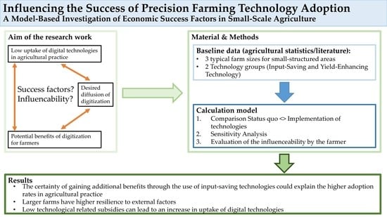
The calculation of the profitability (Equation (1)) of technologies is based on the structure of cost and performance accounting, where direct costs and variable and fixed labor costs are deducted from revenues to determine profit per crop ($P_{cx}$), where the index “cx” describes any field crop. This amount per crop must then be added to total farm profit and is available for the remuneration of the farmland and the farm infrastructure.

$$P_{cx}=R_{cx}-D{C}_{cx}-VO{C}_{cx}-FO{C}_{cx}$$

(1)

The revenue $\left(R_{cx}\right)$ consists of the product of the yield per hectare of a crop and the product price. In order to make the results of the farms comparable, uniform product prices and input prices were used as the basis for the calculation (Table A3). Direct costs $\left(D{C}_{cx}\right)$ include the costs of input use (e.g., fertilizer, seed and pesticide costs). Variable operating costs $(VO{C}_{cx})$ consist of the product of the sum of the operating time of the machines/technologies and the average variable costs per hour. In addition, there may be other variable costs, such as services or labor costs for external employees, which also fall into this category. Fixed operating costs ($FO{C}_{cx}$) include depreciation of machinery, interest costs and costs for family labor. Acquisition costs depreciate on a linear basis over the useful life of the equipment.

$$PC=P_{PFT}-P_{SQ}$$

(2)

The key figure PC (profit change) indicates (Equation (2)) how the farm profit develops at the overall farm level when digital technology is added. The result of the profit change with the use of precision farming technology ($P_{PFT}$) is subtracted from the result of the profit change of the status quo ($P_{SQ}$, without the use of digital technology). All values of the specified indicators in Equations (1)–(3) are given in the unit “Euros per year and farm (€ a⁻¹)”.

$$P_{SQ}<P_{PFT} or PC>0 € a^{-1}$$

(3)

The calculation and selection of technologies are based on the assumption that the farmer makes the decision to use a technology according to the principle of benefit maximization as soon as the additional benefits exceed the additional costs. Such an approach is widely used in the evaluation of digital technologies [1]. From an economic point of view, therefore, investments can be made if Condition (3) is met. The abbreviation “$a$” used in Condition (3) stands for “year”.

The profitability thresholds from Condition (3) served as the starting point for the sensitivity analysis. The aim was to determine whether a change in the variables (listed in

Table 1. Range of data used and ability of the farmer to influence the variables.

Variable	Lower Limit	Upper Limit	Influenceability	References
Changes on revenue side
Natural yield variability	±20%		No	[39,40,41,42,43,44]
Yield change through technology use	0%	4%	Yes	[10,11,32,44,45,46]
Technologically induced product price change	0%	5%	Yes	[11,27,32,43,47,48,49,50,51,52]
Price fluctuations on the market	±10%		No	[39,53,54,55]
Changes on direct cost side
Technologically induced input savings	1%	5%	Yes	[10,11,32,56,57,58]
Input price changes	±10%		No	[33,39,53,55]
European Green Deal (amount of fertilizer)	−20%		No	[35]
Changes on variable operating cost side
Reduction in variable labor costs	0%	4.2%	Yes	[10,11,32,57,58,59]
Changes on fixed operating cost side
Farm size (in ha)	11	303	Yes	Assumption, [36]
Learning costs (deviation from mean)	−50%	+300%	Partially	Assumption based on expert interviews
Investment costs IST (in €)	5150	16,150	Partially	[25,32,58,60,61]
Investment costs YET Farm 1 (in €)	22.986	40.850	Partially	[10,25,37,61,62,63,64]
Investment costs YET Farm 2 (in €)	28.105	51.554	Partially	[10,25,37,61,62,63,64]
Investment costs YET Farm 3 (in €)	31.390	58.424	Partially	[10,25,37,61,62,63,64]
Useful life/depreciation period (deviation from mean)	−50%	+150%	Partially	[32,61]

) had a negative or positive effect on achieving the profitability threshold and the magnitude of the changes caused. For example, it was determined whether a change in the input variable significantly affects the target variable (profitability). The logical conclusion was that variables that are not affected by the farmer and do not cause a significant change in the target variable are negligible. Variables that have a significant effect on the target variable but cannot be directly influenced by the farmer must, for example, become the subject of policy discourse. Input variables that can be influenced but cannot cause a significant change in the target variable are also negligible for the time being.

In contrast, variables that can be influenced or partially influenced and have a significant effect on the target variable point to direct fields of action. This classification of the results of the sensitivity analysis is presented in Section 3.3.

To investigate the influenceability of the variables, a literature review was conducted (Table 1). The calculation of the expected change in the course of technology use was also based on the collected data. Farm size was varied between 11 and 303 ha in the range of Farm 1 and Farm 3, respectively. This range was consistent with the range indicated by other authors as to where the threshold for profitable deployment of these technologies should be sought [33,65]. Technology-related changes (e.g., savings in inputs due to the use of a steering system) and investment costs can be influenced by the farmer’s investment decision. The occurrence of these improvements can be considered certain in most cases since there is no dependence on, e.g., weather conditions. Investment costs can vary depending on the complexity of the technology, status of the existing machinery and size of the machines. Literature values were supplemented by machine prices quoted by manufacturers. However, it can be assumed that the machines will become cheaper over time [32]. For the learning costs (part of the fixed labor costs) and the calibration (for the nitrogen sensor), values based on expert estimates were used, which varied within the above limits. Changes on the variable labor costs side are difficult to map. The level of variable machine costs is technologically determined. Effects are, therefore, mainly conceivable in the area of working time but are very farm specific.

To examine the variables that cannot be influenced by the farmer on the necessary changes in fertilizer quantity and yield, three categories were formed for changes in the product price or input price, respectively. Category 1 included a 10% reduction in the product price and a 10% increase in the fertilizer price. In category 2, the product and fertilizer price remained unchanged from the status quo. For category 3, the product price was increased by 10%, and the fertilizer price was decreased by 10%. In order to classify the magnitude of the shifts of the yield curve “Yield_Status quo” in the Y-direction, limits of natural yield fluctuations from the literature (“Yield_Natural variability_lower limit”, “Yield_Natural variability_upper limit”) were included in the chart. Annual changes in yield of natural origin were known in the range ±20%. These figures can be considered moderate compared to other studies [33,46].

3. Results

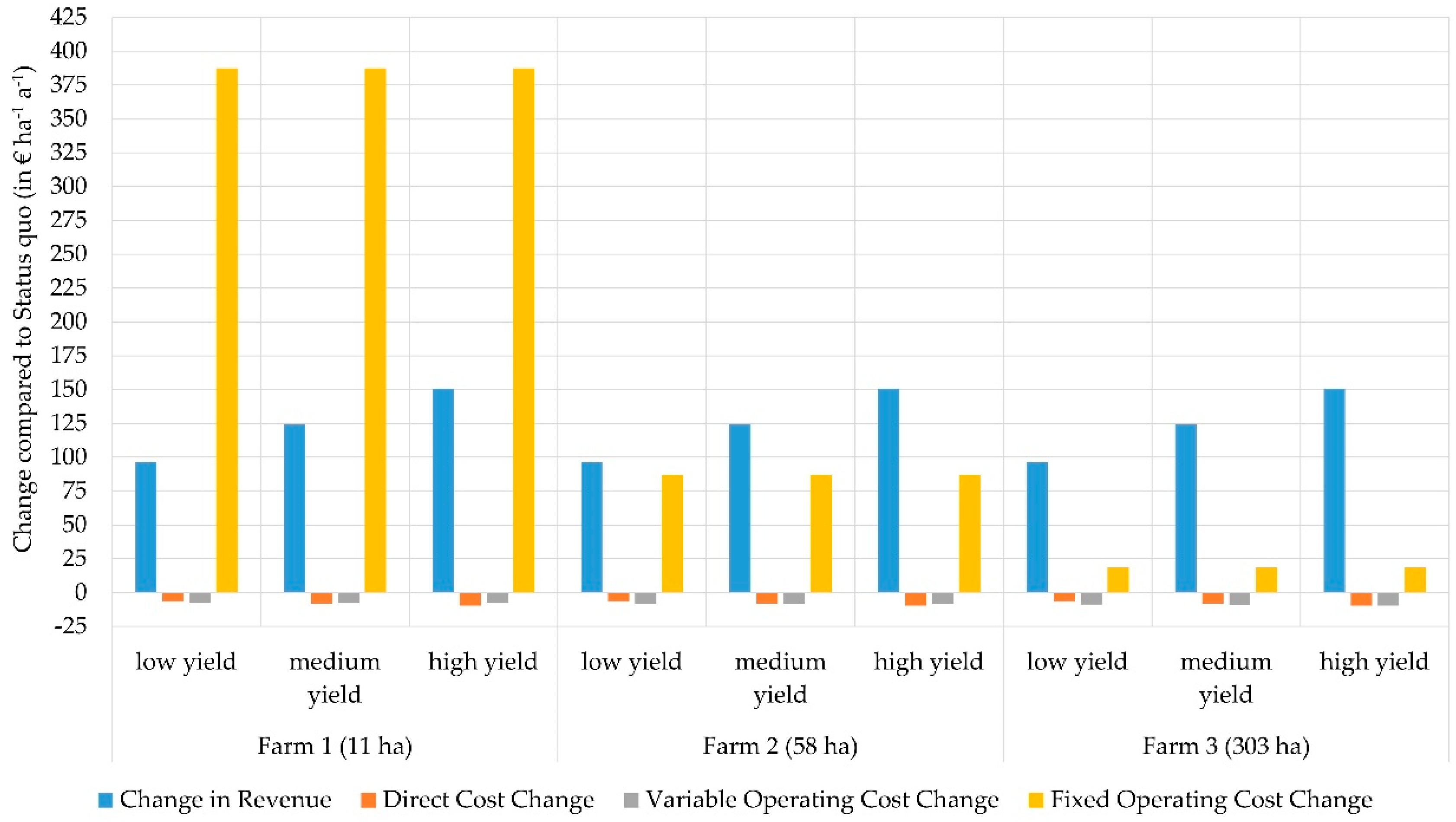
3.1. Input-Saving Technologies (IST)

For the steering assistant, the savings per hectare for each yield level are the same for all farms (Figure 1). There is a difference of 3.7 € ha⁻¹ a⁻¹ between the low yield level (direct cost savings of 7.8 € ha⁻¹ a⁻¹) and the high yield level (direct cost savings of 11.5 € ha⁻¹ a⁻¹). Time savings from less overlap do not translate into savings in variable operating costs. On the one hand, this is due to the already efficient management (only 0.1–0.2 h ha⁻¹ a⁻¹ reduction in field labor time), and, on the other hand, the average variable machine costs per hour increase slightly, so the product of labor time and variable costs per hour actually becomes larger (additional variable labor costs of 1.0 € ha⁻¹ a⁻¹ on Farm 3 to 4.3 € ha⁻¹ a⁻¹ on Farm 1). The revenue side cannot be changed by this technology.

On the additional costs side, high additional fixed labor costs are incurred in addition to a small share of additional variable labor costs, depending on the farm size. Since the retrofittability of the steering assistants (applicable for all tractors) does not lead to a differentiation of the acquisition costs according to farm size or working width, Farm 1, with 103.9 € ha⁻¹ a⁻¹ per hectare, is more financially affected than Farm 2 (18.7 € ha⁻¹ a⁻¹) or Farm 3 (2.5 € ha⁻¹ a⁻¹). Investment costs are also independent of the intensity of farming, so the acquisition costs per hectare remain unchanged for Farm 1 even at the medium or high yield level. The acquisition costs of the steering assistant used in the calculation model amount to EUR 9192 and represent the arithmetic mean of eight steering assistants (EUR 4000–15,000). The learning costs were set at EUR 150. This corresponds to about one hour per year (with a useful life of 10 years and a wage rate of 15 € h⁻¹).

Overall, the positive effect from an economic point of view is very small, which reveals the fact that it is mainly larger farms that use this technology. To a small extent, the yield level or management intensity can increase the benefit. However, the influence of the size of the farm or the area used seems to be the decisive factor for success and is therefore examined in Section 3.2.

3.2. Yield-Enhancing Technologies (YET)

In the case of yield-enhancing technologies, the added benefit is attributable to the increase in revenue and small reductions in direct and variable operating costs (Figure 2). The increase in revenue depends on the yield level and is 96 € ha⁻¹ a⁻¹ at low yield level, 124 € ha⁻¹ a⁻¹ at medium yield level and 151 € ha⁻¹ a⁻¹ at high yield level. Savings in direct costs also depend on yield level and range from 6.4 to 9.6 € ha⁻¹ a⁻¹. The reduction in variable operating costs is mainly due to the higher harvesting capacity of the combine, which can achieve higher throughput in more homogeneous crops. As the larger farms use larger combines, their savings in variable labor costs increase slightly compared to those of Farm 1 (7.1–9.6 € ha⁻¹ a⁻¹).

In this example (Figure 2), the additional costs only include additional fixed operating costs. The acquisition of the technology increases fixed labor costs by 387.5 € ha⁻¹ a⁻¹ for Farm 1, 86.9 € ha⁻¹ a⁻¹ for Farm 2 and 18.4 € ha⁻¹ a⁻¹ for Farm 3. Although a scaling of acquisition costs was made based on farm size (Farm 1, EUR 41,038, Farm 2, EUR 56,604, Farm 3, EUR 66,594 acquisition costs), compared to the additional benefits, the increase in fixed labor costs per hectare is insignificant for Farm 3. Annual learning costs were assumed to be EUR 60 (equivalent to 4 h). Six minutes per hour of usage were planned for the calibration of the sensor.

The analyzed technology leads to an improvement of the profitability compared to the status quo on all farms except Farm 1. It is notable that, in the area of direct costs and variable operating costs, a small improvement is possible for input-saving and yield-enhancing technologies. The reduction of fixed operating costs (mainly influenced by the increase in the farm size) and the change on the revenue side seem to be decisive.

More detailed information on the change in revenue, direct costs, variable and fixed operating costs can be found in the Supplementary Material (Table S1).

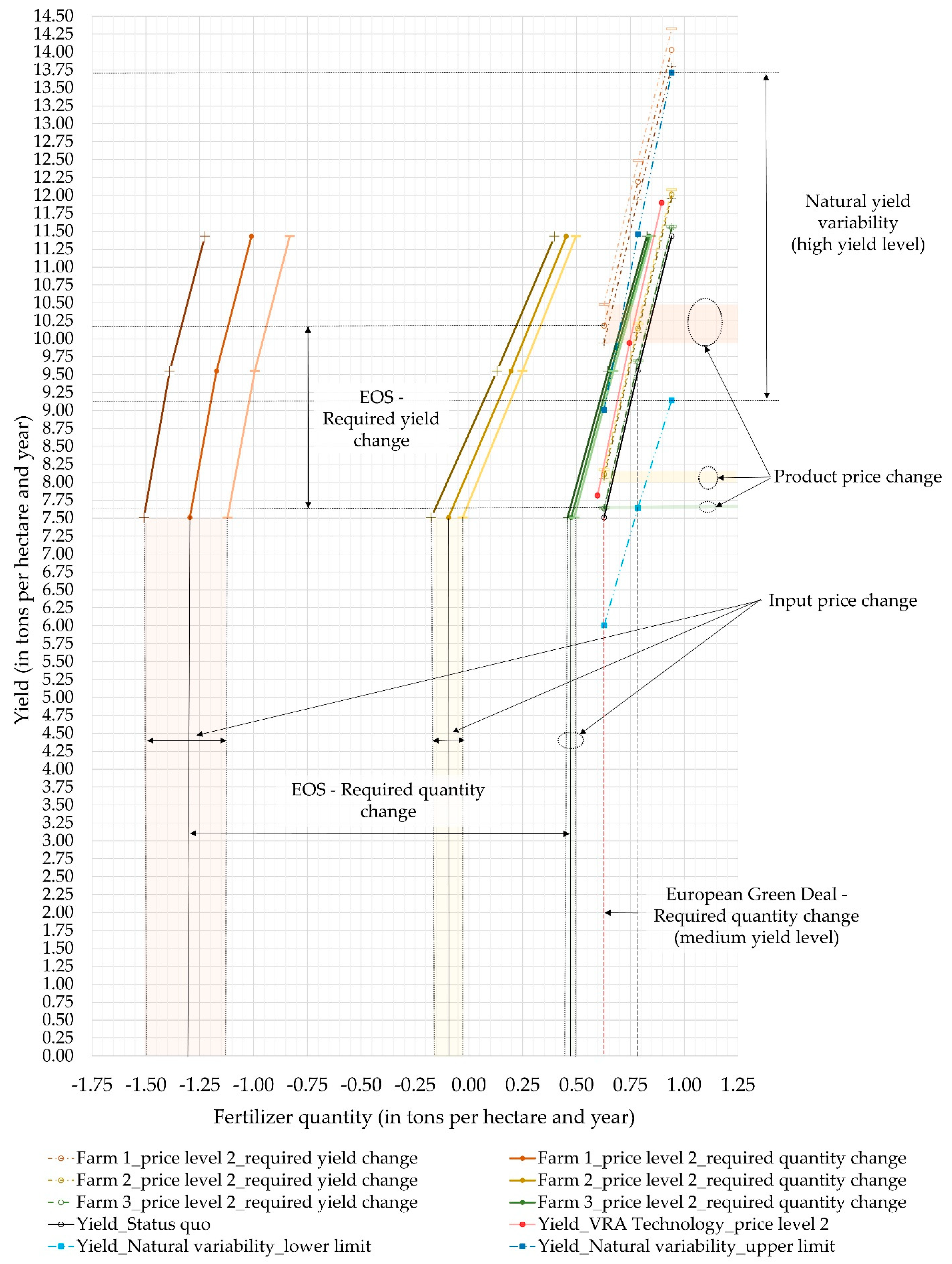
3.3. Sensitivity Analysis

3.3.1. Required Changes in Total Costs and Revenues

To cover additional costs incurred in the course of using the yield-enhancing technology, a reduction in costs or an increase in revenue of 387.5 € ha⁻¹ a⁻¹ is required for Farm 1. This corresponds, for example, to a reduction in fertilizer use of 1.45 t ha⁻¹ a⁻¹ or an increase in yield of 2.01 t ha⁻¹ a⁻¹. For Farm 1, the required reductions in fertilizer are practically impossible, since, even at a high yield level, only 0.94 t ha⁻¹ a⁻¹ of fertilizer is applied. For Farm 2, changes in costs or revenue compared to the status quo of 86.9 € ha⁻¹ a⁻¹ are required, and, for Farm 3, 18.4 € ha⁻¹ a⁻¹ is required to cover the additional costs. This corresponds to a decrease in fertilizer quantity of 0.43 t ha⁻¹ a⁻¹ and 0.09 t ha⁻¹ a⁻¹ and an increase in yield of 0.61 t ha⁻¹ a⁻¹ and 0.12 t ha⁻¹ a⁻¹. When comparing the values to be achieved with the likely shift calculated from literature values, it is noticeable that the main part of the additional benefit is generated from an increase in revenue (96–151 € ha⁻¹ a⁻¹, depending on the yield level) and only a small part (13.9–17.2 € ha⁻¹ a⁻¹) comes from the decrease in costs.

With the steering assistant, lower reductions in input use are necessary compared to those required for the site-specific fertilizer technology due to the lower additional costs. For Farm 1, 108.2 € ha⁻¹ a⁻¹ has to be saved, for Farm 2 21.0 € ha⁻¹ a⁻¹ and for Farm 3 only 3.5 € ha⁻¹ a⁻¹. This corresponds to a decrease in fertilizer use of between 0.55 and 0.02 t ha⁻¹ a⁻¹. The necessary reductions in fertilizer use at Farms 1–2 are, nevertheless, very high in relation to the amount of fertilizer applied in the status quo. However, since this technology is not used exclusively for fertilization, but can be used in all other operations, the necessary savings in direct costs can be generated from a combination of many smaller savings in all the inputs used.

A dependency on size (EOS = economies of scale) is clearly evident in the necessary cost savings or revenue increases, so it can be assumed that the additional costs incurred can be covered sooner as the size of the farm increases.

3.3.2. High Level of Influence—Farm Size

Figure 3 shows the effect of a change in yield level on the minimum required farm size of the steering assistant (red) and the site-specific N fertilization technology (blue). The profitability threshold shown in Section 2.3 is applied, i.e., the technology is implemented as soon as the additional benefits exceed the additional costs. The distance between the functions of the additional costs of the two technologies is 279.3 € ha⁻¹ a⁻¹ for Farm 1 and decreases to 14.9 € ha⁻¹ a⁻¹ for Farm 3, although a differentiation of the acquisition costs according to the farm size was made for the site-specific fertilizer technology, and, thus, Farm 3 is more burdened at the farm level compared to the other farms. The functions of additional benefit are at a low level overall for the steering assistant (7.8 € ha⁻¹ a⁻¹ at the low yield level, 11.5 € ha⁻¹ a⁻¹ at the high yield level), since only a small number of farm inputs can be saved here. For site-specific N fertilization, the benefit function ranges between 109.9 € ha⁻¹ a⁻¹ and 170.1 € ha⁻¹ a⁻¹ depending on the yield level.

For the low yield level, the required acreage for the steering assistant is 148.7 ha, for the medium yield level 118.1 ha and for the high yield level 100.6 ha. The use of the steering assistant is, therefore, only economically feasible for Farm 3. For the yield-enhancing technology, the marginal farm sizes range from 29.4 ha to 44.8 ha depending on the yield level and are, thus, significantly lower. From an economic point of view, the use of this technology is, therefore, feasible for Farm 2 and Farm 3.

Comparing the slopes of the cost graphs of the YET and the IST, it is noticeable that, for the IST between Farm 2 and Farm 3, a small increase in the benefit function causes a significantly higher decrease in the marginal farm size than is the case for the YET. For example, here, a 17.5 € ha⁻¹ a⁻¹ increase in the benefit function results in a 245 ha decrease in minimal farm size (based on the benefit level necessary to achieve the marginal farm size of 303 ha). In the case of YET, achieving the same decrease in the minimum input area requires a nearly fourfold increase in the benefit (benefit increase of EUR 68.5), i.e., depending on the level of the benefit function, a strong increase in the benefit level does not result in a correspondingly high decrease in the minimum input area. On the one hand, technologies for which the cost line has a flat slope in the range of farm sizes >60 ha can also enable small farms to use the technology economically by slightly increasing the benefit function. Technologies that have an IST cost characteristic can, therefore, be made accessible to very small businesses with small amounts of subsidization. On the other hand, the slope of the cost curve at high benefit values, as observed for YET, is not determinant for the economic use of the technology in smallholder areas (<30 ha) when the expected benefits materialize.

In the course of the structural change in agriculture, it is to be expected that smaller farms (<60 ha) can reach the required minimum farm size when changing the farm size due to the steepness of the cost function in the range of 0–60 ha and, thus, participate in the technological transformation of agriculture. An increase in farm size is always beneficial and is independent of external factors (e.g., weather).

3.3.3. Limited Level of Influence—Acquisition, Learning Costs and Depreciation Period

This subchapter acts as a transition between the variables that can be influenced by the farmer and those that cannot be influenced by the farmer. The depreciation period was varied between a reduction by half and an increase by one and a half times the initial value. The lower value represented farms that either buy used machinery and, therefore, can no longer assume the original depreciation period (usually 10 years) or farms that shorten the depreciation period due to a higher usage of the machinery. The upper value can be used primarily for small farms that achieve a longer useful life due to the low degree of utilization of the machines.

For the learning costs, which can vary greatly depending on the digital competence of the farmer, it was assumed that an “expert” only needs half of the average learning time. It was determined in the analysis that farmers who are not at all familiar with digital technologies have to spend three times the average time for initial training (see

Table 2. Changes in the fixed technology costs of the input-saving and yield-enhancing technology (IST/YET) with changes in the acquisition cost, learning cost and depreciation period.

		Fixed Technology Costs ha−1 a−1
		Input-Saving Technology			Yield-Enhancing Technology
		Farm 1	Farm 2	Farm 3	Farm 1	Farm 2	Farm 3
Aquisition costs	low	46.2	8.9	1.7	263.0	68.8	15.2
	medium	92.7	18.0	3.4	372.2	98.3	21.9
	high	144.8	28.1	5.3	473.9	129.0	29.0
Learning costs	low	92.0	17.8	3.4	367.9	97.5	21.7
	medium	92.7	18.0	3.4	372.2	98.3	21.9
	high	95.4	18.5	3.5	389.4	101.7	22.5
Depreciation period	low	175.1	33.9	6.4	729.4	193.8	43.2
	medium	92.7	18.0	3.4	372.2	98.3	21.9
	high	65.2	12.6	2.4	253.2	66.5	14.8

).

The limits of the acquisition costs were based on values from the literature research. The value of the lowest-priced technology available on the market served as the lower limit and the most expensive one as the upper limit.

When comparing the variables “Acquisition costs”, “Learning costs” and “Depreciation period”, it is noticeable that greater advantages on the side of the fixed operating costs only arise with changes in acquisition costs and useful life. For example, if Farm 1 purchases an inexpensive IST, this can mean a benefit of up to 98.6 € ha⁻¹ a⁻¹. A similar situation can be seen on the YET side, where differences of up to 210.9 € ha⁻¹ a⁻¹ occur on Farm 1. It is noteworthy, here, that the differences become smaller the larger the farm is, and Farm 3 would incur, at most, 13.8 € ha⁻¹ a⁻¹ higher costs for YET should the most expensive, available variant be purchased.

The increase in learning costs has only a small influence on the economic success of a technology (maximum 21.5 € ha⁻¹ a⁻¹ difference between a low and high learning effort for YET and Farm 1). Overall, the share of learning costs in technology costs is very low (0.9–1.5%) and, thus, from an economic point of view, not the decisive determinant for the success of a digital technology. When comparing the technologies, it is noticeable that familiarization with YET is more time consuming. This is due to the higher complexity of the technology and the combination of the N sensor and fertilizer spreader.

An increase in the depreciation period has the same effect as a reduction in acquisition costs; however, this change is associated with a higher degree of uncertainty. For many technologies, there are still no empirical values for the maximum useful life, and it is uncertain to what extent older technologies can be supplied with the necessary software updates, spare parts and services. Reducing the annual costs per hectare by increasing the useful life alone seems to be an uncertain method, especially since small farms have a disadvantage in terms of economies of scale and would not be able to cover the additional costs due to the use of the technology even with an increase in depreciation period.

3.3.4. No Influence—Price Changes, Natural Yield Variability and Regulations

To examine the variables that cannot be influenced by the farmer in relation to the necessary changes in fertilizer quantity and yield (Figure 4), three categories were formed for changes in the product price or input price based on the values from the literature (see Section 2.3). For reasons of clarity, the values of the steering assistant were not shown, which, as described in Section 3.1, only led to a reduction in direct costs. At price level 1, there is a reduction in the product price and an increase in the fertilizer price. At price level 2, prices remain unchanged compared to the status quo. At price level 3, the product price is increased, and the fertilizer price is reduced (detailed results in Appendix A 

Table A4. Results of sensitivity analysis—required shifts in product functions on Farms 1–3.

			Yield Level
			Low	Medium	High
Farm 1	Required Yield	Category 1 *	10.48	12.48	14.32
		Category 2 **	10.18	12.19	14.03
		Category 3 ***	9.94	11.95	13.79
	Required Input Quantity	Category 1	−1.51	−1.39	−1.23
		Category 2	−1.30	−1.17	−1.01
		Category 3	−1.12	−0.99	−0.83
Farm 2	Required Yield	Category 1	8.17	10.21	12.08
		Category 2	8.11	10.14	12.01
		Category 3	8.05	10.09	11.96
	Required Input Quantity	Category 1	−0.17	0.13	0.40
		Category 2	−0.09	0.20	0.45
		Category 3	−0.03	0.25	0.50
Farm 3	Required Yield	Category 1	7.65	9.69	11.57
		Category 2	7.63	9.68	11.55
		Category 3	7.62	9.66	11.54
	Required Input Quantity	Category 1	0.46	0.65	0.83
		Category 2	0.48	0.66	0.84
		Category 3	0.49	0.67	0.85
Status quo		Fertilizer Quantity	0.63	0.78	0.94
		Yield	7.51	9.55	11.43
Technology-induced changes		Fertilizer Quantity	0.60	0.75	0.89
		Yield	7.81	9.94	11.90
Natural yield variability		Lower Limit	6.01	7.64	9.14
		Upper Limit	9.01	11.46	13.71

* 10% reduction in product price, 10% increase in input price, ** product and fertilizer price unchanged from status quo, *** 10% increase in product price, 10% decrease in input price.

).

To illustrate the influence of farm size on the shifts due to price changes, the necessary shifts in the yield function for Farms 1–3 are shown in Figure 4 (orange = Farm 1, yellow = Farm 2, green = Farm 3).

If the additional costs have to be compensated only by decreasing the amount of fertilizer, the amount of fertilizer to be saved has to decrease by 1.96 t ha⁻¹ a⁻¹ compared to the value of price level 2 for Farm 1. For Farm 2, this results in a maximum deviation of 0.59 t ha⁻¹ a⁻¹. For Farm 3, there is only a deviation of 0.12 t ha⁻¹ a⁻¹ from price level 2.

The necessary shift of the yield curve in the Y-direction is a maximum of 2.64 t ha⁻¹ a⁻¹ for Farm 1, 0.59 t ha⁻¹ a⁻¹ for Farm 2 and 0.13 t ha⁻¹ a⁻¹ for Farm 3 in the case of the product price fluctuations described above.

For Farm 1, price changes can cause a shift in the yield curve in the X-direction by up to 0.39 t ha⁻¹ a⁻¹. For Farm 2, this value is reduced to 0.11 t ha⁻¹ a⁻¹. For Farm 3, a change in prices requires this shift to be only 0.03 t ha⁻¹ a⁻¹. It can be concluded that increases in farm size have a much larger effect on the economic success of technology use than changes in product and input prices that cannot be influenced. Price-related ranges of variation become smaller the larger the farm. This means that larger farms have a higher resilience to market changes due to the economies of scale of additional costs.

Overall, at price level 3 (product price increase, input price decrease), the yield curves that have to be reached for profitable use of the technology move towards the initial yield curve. Reaching the profitability threshold then seems more likely.

The theoretically calculated necessary shifts of the yield curve in the X-direction have no practical significance for Farm 1 and Farm 2. Savings that are higher than the applied amount per hectare or that deviate very strongly from the application rate of the status quo are not feasible. Since the technology used realizes the additional benefit from an increase in yield, and, at the same time, a reduction in fertilizer quantity, these values are, in any case, redundant.

For a comparison of the fluctuations caused by the product price changes and farm size changes, naturally occurring yield variabilities known from the literature are shown (“Yield_Natural variability_lower limit”, “Yield_Natural variability_upper limit”). At the medium yield level, annual fluctuations of 2.0 t ha⁻¹ a⁻¹ around the value of the status quo can occur.

The factor of a change in the regulatory conditions, which cannot be influenced by the farmer, is shown in Figure 4 on the basis of a 20% reduction in the amount of fertilizer (by 2030) required by the European Green Deal (Farm to Fork Strategy). In this example, legal regulations are straight lines parallel to the Y-axis. They cut off the possibility (regardless of farm size) of reaching a higher yield level by increasing the amount of fertilizer and, thus, achieving higher yields. At the medium yield level, this means a decrease of 0.16 t ha⁻¹ a⁻¹ in fertilizer and 2.0 t ha⁻¹ a⁻¹ in yield. By using the steering assistant, 0.04 t ha⁻¹ a⁻¹ of the amount of fertilizer can be saved without having to accept a loss of yield. Achieving the required maximum amount of fertilizer of 0.63 t ha⁻¹ a⁻¹ means a reduction in yield of 1.8 t ha⁻¹ a⁻¹ despite technology use. In comparison, using yield-enhancing technology reduces yield by only 1.3 t ha⁻¹ a⁻¹ due to the additional shift of the original yield function in the positive Y-direction. Overall, these legal regulations favor either farms that experience a large positive change in profit through technology use (i.e., large and intensive farms) or technologies that can shift the yield function in the positive Y-direction in addition to saving fertilizer (yield-enhancing technologies).

4. Discussion

4.1. Yield-Enhancing Technologies Compared to Input-Saving Technologies

The selection of the steering assistant as an input-saving technology conceals the fact that, above all, more precise automatic steering systems cannot be changed between tractor units but are permanently installed. When using an automatic steering system, it must, therefore, be taken into account that, although the accuracy of work execution can increase and, therefore, more inputs can be saved, higher acquisition costs must also be expected, and the area of utilization is reduced due to tractor-bound use, i.e., the additional costs per hectare increase. The same would happen if Farm 3 were to purchase two steering assistants due to its farm size. Since, in this calculation model, only 3.4 € ha⁻¹ a⁻¹ in additional costs is incurred by Farm 3 due to the use of the input-saving technology, which are offset by a benefit of 7.8–11.5 € ha⁻¹ a⁻¹, the investment in a second steering system would be possible in this case.

With the help of the model calculation, it was demonstrated that yield-enhancing technologies can also be used by small farms (>29.4 ha) due to the high additional benefits. However, the adoption rates of these technologies in agricultural practice compared to steering technologies reflect a different picture. Through a survey in Bavaria (similar structures as in BW), it was shown that steering systems are far more widespread (17%) than site-specific fertilization (less than 5%) [17]. Other studies assumed a similar distribution [16]. It can be concluded that investment decisions in digital technologies also depend on other factors. In the case of steering systems in particular, there are benefits that cannot be assessed economically, such as a reduction in driver fatigue [8,57]. Certainty of benefit attainment can also be a determining factor. Additional benefits can be achieved more reliably by saving the number of inputs to a certain extent than by increasing the yield, which depends on many variables beyond the farmer’s control [25,44]. Another factor can be the complexity of the technology and, thus, the time and effort required for training, which, in the case of guidance systems, can be classified as significantly lower than that required in the case of site-specific fertilization [66]. Although learning costs were included in the calculation, they can vary greatly based on the level of knowledge of the farm managers [9,26]. Lastly, GPS guidance systems can be seen as a key technology for moving into precision farming and, therefore, are probably often a farm’s first technology [18].

In the case of yield-enhancing technologies, which generate most of the additional benefit from increased yield, it should be noted that the production functions of the individual fields or plots are usually not known to the farmer, and, therefore, no reliable statements can be made about how a change in the amount of fertilizer affects the level of yield. The same applies to the yield functions shown and the necessary shifts in the input-saving technologies. It is unlikely, however, that the necessary reductions in inputs to reach the profitability threshold can be achieved, especially on Farm 1, without causing a reduction in yield.

Since the focus of the present work was on the investigation of effects in small-scale agriculture, the limited scope of the study (11–303 ha in three stages) leaves open questions about larger structures or intermediate stages. In a further step, it would, therefore, be interesting to investigate whether (a) farm sizes between the mentioned sizes (11 ha, 58 ha, 303 ha) react differently to the selected effects and (b) farms in larger structured regions of the world (e.g., Eastern Europe or South America) are always at an advantage or whether stepped fixed costs and other effects can also negatively influence profitability there. A further step in a more application-oriented direction would be to extend the investigation beyond the two technology groups mentioned above to all precision agriculture technologies available to date. Furthermore, it would be interesting to investigate path dependencies, for example, whether differences in profitability arise if different degrees of digitization of the farms are assumed or if several technologies are purchased at once.

4.2. Sensitivity Analysis—Influenceable Factors

The factor of farm size increase, which is described by the farmer as influenceable, can, in reality, only be changed within certain limits. Although favorable side effects can be seen, especially in small-structured areas (structural change), the increases in farm size required by input-saving technology cannot be achieved without major restructuring efforts (e.g., adaptation of the entire fleet of machinery). Farm 1 would have to increase the farm area by up to 137.5 ha, depending on the yield level, which is a 1327% change from the status quo. Apart from the fact that sharing a steering system cannot be considered reasonable, more than thirteen farms of the size of Farm 1 would have to cooperate to reach the profitability threshold. Kutter et al. [26] observed a general reluctance of farmers to make joint investments. Nevertheless, increasing the size of the farm is the most effective lever for keeping the additional cost per hectare low. This is an opportunity, especially for service providers, to use new technologies in a profitable way [56]. However, a positive profit change compared to the status quo will only occur on the farms if the advantage of the economies of scale in machine costs is passed on from the service provider to the farmer. The risk of achieving the benefits to cover the additional costs of the digital technology, especially in the case of yield-enhancing technology, is entirely on the side of the farmer, so this technology will only become established if either the costs are correspondingly low (e.g., also through a subsidy per hectare of land cultivated with digital technologies) or the achievement of a sufficient benefit is certain [67].

The reduction in the use of inputs, especially when GPS guidance systems are used, is technologically determined (less overlap) and can, therefore, be regarded by the farmer as safely achievable. In addition, the reduction in overlap depends on the steering system and GPS signal used and can, therefore, also be controlled by the farmer in terms of the amount through the investment decision [9]. Nevertheless, the necessary reduction in input use must be seen in relation to the probable reduction (shift of the original production function, calculated from literature values). A reduction in input use of 108.2 € ha⁻¹ a⁻¹ on Farm 1 can be considered unlikely compared to the values known from the literature (1–5% saving in inputs, Table 1).

When choosing the manufacturer of a technology, the farmer can usually choose freely and, thus, theoretically select the most cost-effective one. The prerequisite in this case, however, is that all choices have the same characteristics and equipment variants. In practice, this is not the case and would require time-consuming research work on the part of the farmer. A farmer, therefore, usually selects from among known dealers in his region and is thus limited in choice [26]. Not to be underestimated in this regard, are the different user interfaces and user-friendliness of the various manufacturers, so the choice can also depend on the manufacturer being known to the farmer. Therefore, in most cases, the acquisition costs and associated learning costs are only under the control of the farmer to a limited extent.

In addition, much of the learning effort typically falls in the year of acquisition because, for example, technologies must be installed, and the basic functions of the technology must be learned. This assumption was supported by Tey and Brindal [1]. Since, in this calculation, the learning costs depreciate on a linear basis over the lifetime of the technology, the actual effort required for familiarization in the first year of use is underestimated. This is probably one of the reasons why farmers hesitate to invest in digital technologies, knowing that additional expenditure in the year of acquisition can lead to capacity shortages on the farm [19,32]. In addition, the training effort is determined by the existing mechanization. If, for example, only software updates are necessary, the effort is considerably less than that required for a complex retrofit or new purchase. Easy-to-use technologies that work according to the plug-and-play principle would be helpful in this context. Here, manufacturers are called upon to create user-friendly interfaces and promote compatibility among technologies [68]. The assumption that different labor capacities lead to different implementation successes was not investigated in this study and should be the subject of future research. It can be assumed that farms with a higher labor capacity are more flexible and can implement more successfully or more quickly.

In the calculation model, the maximum depreciation period used was 10 years. Some economic studies have suggested that the useful life can vary between 5 and 20 years, depending on the technology [32]. To date, there is no practice-oriented assessment of the useful life of digital technologies, as the figures used are assumptions. The ability of small businesses to reduce the annual depreciation rate by using the technologies for a long time is, therefore, subject to great uncertainty. From today’s perspective, it is not possible to ensure, for example, whether the necessary software updates will still be available after more than 10 years or whether the software and hardware components used will have a correspondingly long service life.

The scale of the crops was not changed, although the economic success of the introduction of digital technologies may well depend on the crops grown and their scale [13,69]. This circumstance needs to be investigated in further projects.

4.3. Sensitivity Analysis—Non-Influenceable Factors

Contrary to expectations, price fluctuations for the variation ranges used have a smaller impact on the success of digital technology adoption than an increase in farm size. This would presumably change if fertilizer prices continue to rise or if regulatory requirements necessitate a more efficient distribution of fertilizers [13]. Nevertheless, larger farms show a higher resilience to fluctuations in product and input prices, which are not caused by the yield level or the achievable benefit but by the scale dependency of the additional costs. Possible solutions to enable Farm 2 to increase the application area of the technology are mainly to be seen in machine cooperatives. Farm 1 could use a service provider to carry out site-specific fertilization.

The curves of natural yield variability are based on the assumption that the farmer will not change his management strategy. In fact, especially if it is predictable that a drought period will last longer, he will adapt his management strategy accordingly and, for example, reduce further fertilization measures. The cost savings that can be achieved in this way were not included in Figure 4.

All in all, the indicated reduction of 20% in the amount of fertilizer used (European Green Deal [35]) is a severe cut and would significantly reduce agricultural productivity. Whether a redistribution of the amount of fertilizer (site-specific fertilization) can compensate for the decline in yield is questionable, especially with regard to small-structured areas, which can have small but homogeneous fields. In this case, redistribution would have no effect. It is hoped that the use of other complementary technologies, such as section control and GPS guidance systems, can further reduce fertilizer use to unshaped fields without causing further yield losses. These technologies are already found in many new machines and can, therefore, be used directly without retrofitting.

The factors described as non-influenceable are, to some extent, controllable by adaptation measures and depend on the choice of technology. Yield-enhancing technologies, which aim to generate a large part of the additional benefits by increasing yields, react more sensitively to external, non-influenceable factors than input-saving technologies, which generate additional benefits by increasing the accuracy of work execution.

5. Conclusions

The results of the calculation model show that input-saving technologies are still relatively expensive, and the benefits are low compared to the additional costs. However, since the benefits are relatively independent of external influences, higher adoption rates are observed in agricultural practice than for yield-increasing technologies, the economic parameters of which actually appear more advantageous. Due to the relatively flat slope of the cost curve between 30 and 300 ha and a possible further decrease in investment costs, it is expected that an increasing number of farms will come within the range of the necessary farm size as structural change progresses. Despite very high initial costs, the investigated yield-enhancing technology can also be used profitably by smaller farms (>30 ha) if the assumed benefits can be achieved. Overall, it can be stated that small farms are at a disadvantage due to the scale dependency of the acquisition costs.

A detailed economic analysis of the farm is, in any case, the basis for investment decisions. This work has shown that the level of investment costs, the additional benefits per hectare and, above all, their relationship to each other are decisive for the success of the introduction of a digital technology. Farms interested in adopting digital technologies should, therefore, (a) know their status quo very well (e.g., cost structure of the operation), (b) collect relevant data in sufficient detail even during and after adoption (what changes result from the implementation) and then (c) make changes based on the data collected. Since these steps are often costly in practice, small farms (<30 ha) are advised to use service providers, medium farms (30–70 ha) can join machine pools and, beyond that, government grants can help with the acquisition of these technologies.

Reassuringly, any hesitation among farmers in small-structured areas cannot be attributed to implementation effort (learning costs), as increasing this position is unlikely to affect the economic use of the technologies. Therefore, improving farmers’ digital literacy or the usability of the technologies is not crucial at the moment. A simple entry into the world of digitization in agriculture can be made through service providers who can make digital technologies available on a temporary basis, irrespective of the given mechanization of the farm. Since the small-scale structure of European agriculture will probably not decrease in the coming years to the extent that would be necessary for a broad diffusion of digital technologies in agriculture, this results in special requirements for policy. For technologies with similar cost characteristics to the input-saving technology presented, even a small financial subsidy (<20 € ha) would result in a large proportion of farms reaching the profitability threshold and thus meeting all the conditions for using the technology from an economic perspective. One approach to the main problem of lack of profitability of digital technologies would be to provide financial support to farmers until appropriate cost-effective technologies are available.

References

1. Tey, Y.S.; Brindal, M. Factors influencing the adoption of precision agricultural technologies: A review for policy implications. Precis. Agric. 2012, 13, 713–730. [Google Scholar] [CrossRef]
2. FAO. The Future of Food and Agriculture-Trends and Challenges; FAO: Rome, Italy, 2017. [Google Scholar]
3. Valin, H.; Sands, R.D.; van der Mensbrugghe, D.; Nelson, G.C.; Ahammad, H.; Blanc, E.; Bodirsky, B.; Fujimori, S.; Hasegawa, T.; Havlik, P.; et al. The future of food demand: Understanding differences in global economic models. Agric. Econ. 2014, 45, 51–67. [Google Scholar] [CrossRef]
4. Godfray, H.C.J.; Beddington, J.R.; Crute, I.R.; Haddad, L.; Lawrence, D.; Muir, J.F.; Pretty, J.; Robinson, S.; Thomas, S.M.; Toulmin, C. Food security: The challenge of feeding 9 billion people. Science 2010, 327, 812–818. [Google Scholar] [CrossRef] [Green Version]
5. Värnik, R.; Aste, R.; Ariva, J. Sustainable Intensification in Crop Farming—A Case from Estonia. In Precision Agriculture: Technology and Economic Perspectives; Pedersen, S.M., Lind, K.M., Eds.; Springer: Cham, Switzerland, 2017; pp. 201–221. ISBN 978-3-319-68713-1. [Google Scholar]
6. Bongiovanni, R.; Lowenberg-Deboer, J. Precision Agriculture and Sustainability. Precis. Agric. 2004, 5, 359–387. [Google Scholar] [CrossRef]
7. Zambon, I.; Cecchini, M.; Egidi, G.; Saporito, M.G.; Colantoni, A. Revolution 4.0: Industry vs. Agriculture in a Future Development for SMEs. Processes 2019, 7, 36. [Google Scholar] [CrossRef] [Green Version]
8. Daberkow, S.G.; McBride, W.D. Farm and Operator Characteristics Affecting the Awareness and Adoption of Precision Agriculture Technologies in the US. Precis. Agric. 2003, 4, 163–177. [Google Scholar] [CrossRef]
9. Balafoutis, A.T.; Beck, B.; Fountas, S.; Tsiropoulos, Z.; Vangeyte, J.; van der Wal, T.; Soto-Embodas, I.; Gómez-Barbero, M.; Pedersen, S.M. Smart Farming Technologies–Description, Taxonomy and Economic Impact. In Precision Agriculture: Technology and Economic Perspectives; Pedersen, S.M., Lind, K.M., Eds.; Springer: Cham, Switzerland, 2017; pp. 21–77. ISBN 978-3-319-68713-1. [Google Scholar]
10. Heege, H.J. (Ed.) Precision in Crop Farming: Site Specific Concepts and Sensing Methods: Applications and Results; Springer: Dordrecht, The Netherlands, 2013; ISBN 9789400767607. [Google Scholar]
11. Chen, W.; Bell, R.W.; Brennan, R.F.; Bowden, J.W.; Dobermann, A.; Rengel, Z.; Porter, W. Key crop nutrient management issues in the Western Australia grains industry: A review. Soil Res. 2009, 47, 1. [Google Scholar] [CrossRef]
12. Michalski, A.; Czajewski, J. Instrumentatio nnotes-The accuracy of the global positioning systems. IEEE Instrum. Meas. Mag. 2004, 7, 56–60. [Google Scholar] [CrossRef]
13. Paustian, M.; Theuvsen, L. Adoption of precision agriculture technologies by German crop farmers. Precis. Agric. 2017, 18, 701–716. [Google Scholar] [CrossRef]
14. Reichardt, M.; Jürgens, C.; Klöble, U.; Hüter, J.; Moser, K. Dissemination of precision farming in Germany: Acceptance, adoption, obstacles, knowledge transfer and training activities. Precis. Agric. 2009, 10, 525–545. [Google Scholar] [CrossRef]
15. Bramley, R.G.V. Lessons from nearly 20 years of Precision Agriculture research, development, and adoption as a guide to its appropriate application. Crop Pasture Sci. 2009, 60, 197. [Google Scholar] [CrossRef]
16. Lowenberg-DeBoer, J.; Erickson, B. Setting the Record Straight on Precision Agriculture Adoption. Agron. J. 2019, 111, 1552–1569. [Google Scholar] [CrossRef] [Green Version]
17. Gabriel, A.; Gandorfer, M. Landwirte-Befragung 2020 Digitale Landwirtschaft Bayern. 2020. Available online: https://www.lfl.bayern.de/mam/cms07/ilt/dateien/ilt6_praesentation_by_2390_27082020.pdf (accessed on 24 September 2022).
18. Groher, T.; Heitkämper, K.; Walter, A.; Liebisch, F.; Umstätter, C. Status quo of adoption of precision agriculture enabling technologies in Swiss plant production. Precis. Agric. 2020, 21, 1327–1350. [Google Scholar] [CrossRef]
19. Aubert, B.A.; Schroeder, A.; Grimaudo, J. IT as enabler of sustainable farming: An empirical analysis of farmers' adoption decision of precision agriculture technology. Decis. Support Syst. 2012, 54, 510–520. [Google Scholar] [CrossRef] [Green Version]
20. Tamirat, T.W.; Pedersen, S.M.; Lind, K.M. Farm and operator characteristics affecting adoption of precision agriculture in Denmark and Germany. Acta Agric. Scand. Sect. B Soil Plant Sci. 2018, 68, 349–357. [Google Scholar] [CrossRef]
21. Kernecker, M.; Knierim, A.; Wurbs, A.; Kraus, T.; Borges, F. Experience versus expectation: Farmers’ perceptions of smart farming technologies for cropping systems across Europe. Precis. Agric. 2020, 21, 34–50. [Google Scholar] [CrossRef]
22. Schimmelpfennig, D. Farm Profits and Adoption of Precision Agriculture. 2016. Available online: https://www.researchgate.net/publication/309565269_Farm_Profits_and_Adoption_of_Precision_Agriculture (accessed on 24 September 2022).
23. Mondal, P.; Basu, M. Adoption of precision agriculture technologies in India and in some developing countries: Scope, present status and strategies. Prog. Nat. Sci. 2009, 19, 659–666. [Google Scholar] [CrossRef]
24. Bovensiepen, G.; Hombach, R. Quo Vadis, Agricola? Smart Farming: Nachhaltigkeit und Effizienz Durch den Einsatz Digitaler Technologien. 2016. Available online: https://www.pwc.de/de/handel-und-konsumguter/assets/smart-farming-studie-2016.pdf (accessed on 24 September 2022).
25. Robertson, M.; Isbister, B.; Maling, I.; Oliver, Y.; Wong, M.; Adams, M.; Bowden, B.; Tozer, P. Opportunities and constraints for managing within-field spatial variability in Western Australian grain production. Field Crops Res. 2007, 104, 60–67. [Google Scholar] [CrossRef]
26. Kutter, T.; Tiemann, S.; Siebert, R.; Fountas, S. The role of communication and co-operation in the adoption of precision farming. Precis. Agric. 2011, 12, 2–17. [Google Scholar] [CrossRef]
27. Gandorfer, M.; Meyer-Aurich, A. Economic Potential of Site-Specific Fertiliser Application and Harvest Management. In Precision Agriculture: Technology and Economic Perspectives; Pedersen, S.M., Lind, K.M., Eds.; Springer: Cham, Switzerland, 2017; pp. 79–92. ISBN 978-3-319-68713-1. [Google Scholar]
28. Robertson, M.J.; Llewellyn, R.S.; Mandel, R.; Lawes, R.; Bramley, R.G.V.; Swift, L.; Metz, N.; O’Callaghan, C. Adoption of variable rate fertiliser application in the Australian grains industry: Status, issues and prospects. Precis. Agric. 2012, 13, 181–199. [Google Scholar] [CrossRef]
29. Waltmann, M.; Gindele, N.; Doluschitz, R. Informatik in der Land-, Forst- und Ernährungswirtschaft, (S. 275-280): Fokus: Digitalisierung für Landwirtschaftliche Betriebe in Kleinstrukturierten Regione-ein Widerspruch in Sich?: Referate der 39. GIL-Jahrestagung 18.-19. Februar 2019 Wien, Österreich; Meyer-Aurich, A., Gandorfer, M., Barta, N., Gronauer, A., Kantelhardt, J., Floto, H., Eds.; Gesellschaft für Informatik e.V: Bonn, Germany, 2019; ISBN 9783885796817. [Google Scholar]
30. Jensen, H.G.; Jacobsen, L.-B.; Pedersen, S.M.; Tavella, E. Socioeconomic impact of widespread adoption of precision farming and controlled traffic systems in Denmark. Precis. Agric. 2012, 13, 661–677. [Google Scholar] [CrossRef]
31. Lambert, D.M.; Lowenberg-DeBoer, J.; Griffin, T.W.; Peone, J.; Payne, T.; Daberkow, S.G. Adoption, Profitability, and Making Better Use of Precision Farming Data; Dept. of Agricultural Economics, Purdue University: West Lafayette, Indiana, 2004. [Google Scholar]
32. Jochinke, D.C.; Noonon, B.J.; Wachsmann, N.G.; Norton, R.M. The adoption of precision agriculture in an Australian broadacre cropping system—Challenges and opportunities. Field Crops Res. 2007, 104, 68–76. [Google Scholar] [CrossRef]
33. Lawes, R.A.; Robertson, M.J. Whole farm implications on the application of variable rate technology to every cropped field. Field Crops Res. 2011, 124, 142–148. [Google Scholar] [CrossRef]
34. Finger, R.; Swinton, S.M.; El Benni, N.; Walter, A. Precision Farming at the Nexus of Agricultural Production and the Environment. Annu. Rev. Resour. Econ. 2019, 11, 313–335. [Google Scholar] [CrossRef] [Green Version]
35. European Commission. Farm to Fork Strategy-for a Fair, Healthy and Environmentally-Friendly Food System. 2020. Available online: https://food.ec.europa.eu/horizontal-topics/farm-fork-strategy_en (accessed on 24 September 2022).
36. Statistisches Landesamt BW. Landwirtschaftszählung 2020 in Baden-Württemberg-Aus der Reihe Statistische Daten; Statistisches Landesamt Baden-Württemberg: Stuttgart, Germany, 2021.
37. Kuratorium für Technik und Bauwesen in der Landwirtschaft e.V. Leistungs-Kostenrechnung Pflanzenbau. Available online: https://daten.ktbl.de/dslkrpflanze/postHv.html (accessed on 24 September 2022).
38. Schimmelpfennig, D.; Ebel, R. Sequential Adoption and Cost Savings from Precision Agriculture. J. Agric. Resour. Econ. 2016, 41, 97–115. [Google Scholar]
39. Karatay, Y.N.; Meyer-Aurich, A. Profitability and downside risk implications of site-specific nitrogen management with respect to wheat grain quality. Precis. Agric. 2020, 21, 449–472. [Google Scholar] [CrossRef]
40. Whelan, B.M.; McBratney, A.B. The “Null Hypothesis” of Precision Agriculture Management. Precis. Agric. 2000, 2, 265–279. [Google Scholar] [CrossRef]
41. Robertson, M.J.; Lyle, G.; Bowden, J.W. Within-field variability of wheat yield and economic implications for spatially variable nutrient management. Field Crops Res. 2008, 105, 211–220. [Google Scholar] [CrossRef] [Green Version]
42. Statistisches Landesamt BW. Ertragsentwicklung Ausgewählter Feldfrüchte 1988–2021. Available online: https://www.statistik-bw.de/Landwirtschaft/Ernte/Feldfruechte-LR-1988.jsp (accessed on 24 September 2022).
43. Morari, F.; Zanella, V.; Sartori, L.; Visioli, G.; Berzaghi, P.; Mosca, G. Optimising durum wheat cultivation in North Italy: Understanding the effects of site-specific fertilization on yield and protein content. Precis. Agric. 2018, 19, 257–277. [Google Scholar] [CrossRef]
44. Basso, B.; Cammarano, D.; Fiorentino, C.; Ritchie, J.T. Wheat yield response to spatially variable nitrogen fertilizer in Mediterranean environment. Eur. J. Agron. 2013, 51, 65–70. [Google Scholar] [CrossRef]
45. Colaço, A.F.; Bramley, R. Do crop sensors promote improved nitrogen management in grain crops? Field Crops Res. 2018, 218, 126–140. [Google Scholar] [CrossRef]
46. Basso, B.; Dumont, B.; Cammarano, D.; Pezzuolo, A.; Marinello, F.; Sartori, L. Environmental and economic benefits of variable rate nitrogen fertilization in a nitrate vulnerable zone. Sci. Total Environ. 2016, 545–546, 227–235. [Google Scholar] [CrossRef] [PubMed] [Green Version]
47. Gandorfer, M.; Rajsic, P. Modeling Economic Optimum Nitrogen Rates for Winter Wheat When Inputs Affect Yield and Output-Price. Agric. Econ. Rev. 2008, 9, 54–63. [Google Scholar]
48. Long, D.S.; Engel, R.E.; Carlson, G.R. Method for Precision Nitrogen Management in Spring Wheat: II. Implementation. Precis. Agric. 2000, 2, 25–38. [Google Scholar] [CrossRef]
49. Bongiovanni, R.G.; Robledo, C.W.; Lambert, D.M. Economics of site-specific nitrogen management for protein content in wheat. Comput. Electron. Agric. 2007, 58, 13–24. [Google Scholar] [CrossRef]
50. Meyer-Aurich, A.; Griffin, T.W.; Herbst, R.; Giebel, A.; Muhammad, N. Spatial econometric analysis of a field-scale site-specific nitrogen fertilizer experiment on wheat (Triticum aestuvum L.) yield and quality. Comput. Electron. Agric. 2010, 74, 73–79. [Google Scholar] [CrossRef]
51. Meyer-Aurich, A.; Weersink, A.; Gandorfer, M.; Wagner, P. Optimal site-specific fertilization and harvesting strategies with respect to crop yield and quality response to nitrogen. Agric. Syst. 2010, 103, 478–485. [Google Scholar] [CrossRef]
52. Yost, M.A.; Kitchen, N.R.; Sudduth, K.A.; Massey, R.E.; Sadler, E.J.; Drummond, S.T.; Volkmann, M.R. A long-term precision agriculture system sustains grain profitability. Precis. Agric. 2019, 20, 1177–1198. [Google Scholar] [CrossRef]
53. Havlin, J.L.; Heiniger, R.W. A variable-rate decision support tool. Precis. Agric. 2009, 10, 356–369. [Google Scholar] [CrossRef]
54. European Commission. Price Dashboard No 116-January 2022 Edition. 2022. Available online: https://ec.europa.eu/info/sites/default/files/food-farming-fisheries/farming/documents/commodity-price-dashboard_2022-02_en.pdf (accessed on 24 September 2022).
55. Statistisches Bundesamt. Allgemeine Preisstatistik. Available online: https://www.bmel-statistik.de/preise/allgemeine-preisstatistik#c9447 (accessed on 24 September 2022).
56. Koch, B.; Khosla, R.; Frasier, W.M.; Westfall, D.G.; Inman, D. Economic Feasibility of Variable-Rate Nitrogen Application Utilizing Site-SpecificManagement Zones. Agron. J. 2004, 96, 1572–1580. [Google Scholar] [CrossRef] [Green Version]
57. Shockley, J.M.; Dillon, C.R.; Stombaugh, T.S. A Whole Farm Analysis of the Influence of Auto-Steer Navigation on Net Returns, Risk, and Production Practices. J. Agric. Appl. Econ. 2011, 43, 57–75. [Google Scholar] [CrossRef] [Green Version]
58. Mees, M.; Hedtrich, J. Investitionszyklen bei GPS-Gestützter Technik. Available online: https://llh.hessen.de/unternehmen/unternehmensfuehrung/analyse-strategie-und-finanzen/investitionszyklen-bei-gps-gestuetzter-technik/ (accessed on 24 September 2022).
59. Sørensen, C.G.; Rodias, E.; Bochtis, D. Auto-Steering and Controlled Traffic Farming–Route Planning and Economics. In Precision Agriculture: Technology and Economic Perspectives; Pedersen, S.M., Lind, K.M., Eds.; Springer: Cham, Switzerland, 2017; pp. 129–145. ISBN 978-3-319-68713-1. [Google Scholar]
60. Treiber-Niemann, H.; Schwaiberger, R.; Fröba, N.; Kloepfer, F. (Eds.) Parallelfahrsysteme; KTBL: Darmstadt, Germany, 2013; ISBN 9783941583849. [Google Scholar]
61. Achilles, W.; Anter, J.; Belau, T.; Blankenburg, J. (Eds.) Faustzahlen Für Die Landwirtschaft; Kuratorium für Technik und Bauwesen in der Landwirtschaft e.V. (KTBL): Darmstadt, Germany, 2018; ISBN 9783945088593. [Google Scholar]
62. van Henten, E.J.; Goense, D.; Lokhorst, C. Precision Agriculture’09; Wageningen Academic Publishers: Wakhningen, The Netherlands, 2009; ISBN 978-90-8686-113-2. [Google Scholar]
63. Drücker, H. (Ed.) Precision Farming-Sensorgestützte Stickstoffdüngung; KTBL: Darmstadt, Germany, 2016. [Google Scholar]
64. Reckleben, Y.; Schneider, M.; Wagner, P.; Schwarz, J.; Hüter, J. Teilflächenspezifische Stickstoffdüngung; Kuratorium für Technik und Bauwesen in der Landwirtschaft: Darmstadt, Germany, 2007; ISBN 9783939371519. [Google Scholar]
65. Godwin, R.; Richards, T.; Wood, G.; Welsh, J.; Knight, S. An Economic Analysis of the Potential for Precision Farming in UK Cereal Production. Biosyst. Eng. 2003, 84, 533–545. [Google Scholar] [CrossRef]
66. Miller, N.J.; Griffin, T.W.; Ciampitti, I.A.; Sharda, A. Farm adoption of embodied knowledge and information intensive precision agriculture technology bundles. Precis. Agric. 2019, 20, 348–361. [Google Scholar] [CrossRef]
67. Faria, A.; Fenn, P.; Bruce, A. A count Data Model of technology adoption. J. Technol. Transf. 2003, 28, 63–79. [Google Scholar] [CrossRef]
68. Vecchio, Y.; Agnusdei, G.P.; Miglietta, P.P.; Capitanio, F. Adoption of Precision Farming Tools: The Case of Italian Farmers. Int. J. Environ. Res. Public Health 2020, 17, 869. [Google Scholar] [CrossRef] [Green Version]
69. Khanna, M.; Epouhe, O.F.; Hornbaker, R. Site-Specific Crop Management: Adoption Patterns and Incentives. Appl. Econ. Perspect. Policy 1999, 21, 455–472. [Google Scholar] [CrossRef]
70. Ministerium für Ernährung, Ländlichen Raum und Verbraucherschutz-Baden-Württemberg. Betriebswirtschaftliche Ausrichtung-Ergebnisse der Landwirtschaftszählung. 2020. Available online: https://www.landwirtschaft-bw.info/pb/,Lde/3650826_3651462_5405915_5378885_5378985_5401010_5401663 (accessed on 13 October 2022).
71. Statistisches Bundesamt. Land- und Forstwirtschaft, Fischerei-Betriebswirtschaftliche Ausrichtung und Standardoutput Agrarstrukturerhebung. 2017. Available online: https://www.destatis.de/DE/Themen/Branchen-Unternehmen/Landwirtschaft-Forstwirtschaft-Fischerei/Landwirtschaftliche-Betriebe/Publikationen/Downloads-Landwirtschaftliche-Betriebe/betriebswirtschaftliche-ausrichtung-standardoutput-2030214169004.pdf?__blob=publicationFile (accessed on 13 October 2022).
Figure 1. Farm economic changes of the status quo by using an input-saving technology on Farms 1–3 with three different yield levels each (low, medium, high).
Agriculture 12 01773 g001
Figure 2. Farm economic changes of the status quo by using a yield-enhancing technology on Farms 1–3 with three different yield levels each (low, medium, high).
Agriculture 12 01773 g002
Figure 3. Different marginal farm sizes for the use of input-saving and yield-enhancing technologies at certain yield levels.
Agriculture 12 01773 g003
Figure 4. Necessary shift in production functions of Farms 1–3 to cover the additional costs of using the variable-rate technology in the face of changes in product price, input price and natural variation in yields.
Agriculture 12 01773 g004