Estimation of Nitrogen Content in Winter Wheat Based on Multi-Source Data Fusion and Machine Learning

Abstract

Nitrogen (N) is an important factor limiting crop productivity, and accurate estimation of the N content in winter wheat can effectively monitor the crop growth status. The objective of this study was to evaluate the ability of the unmanned aerial vehicle (UAV) platform with multiple sensors to estimate the N content of winter wheat using machine learning algorithms; to collect multispectral (MS), red-green-blue (RGB), and thermal infrared (TIR) images to construct a multi-source data fusion dataset; to predict the N content in winter wheat using random forest regression (RFR), support vector machine regression (SVR), and partial least squares regression (PLSR). The results showed that the mean absolute error (MAE) and relative root-mean-square error (rRMSE) of all models showed an overall decreasing trend with an increasing number of input features from different data sources. The accuracy varied among the three algorithms used, with RFR achieving the highest prediction accuracy with an MAE of 1.616 mg/g and rRMSE of 12.333%. For models built with single sensor data, MS images achieved a higher accuracy than RGB and TIR images. This study showed that the multi-source data fusion technique can enhance the prediction of N content in winter wheat and provide assistance for decision-making in practical production.

1. Introduction

Nitrogen (N) is an essential element for crop growth and development, as well as an important component of chlorophyll, which directly affects photosynthesis in leaves [1]. The inadequate application of N fertilizer can lead to an abnormal growth of winter wheat, resulting in reduced yields [2]. Applying too much N fertilizer causes a waste of resources and environmental pollution [3]. Therefore, early and accurate monitoring of the N content of winter wheat allows for the development of a reasonable fertilizer application program to ensure high yields while reducing resource wastage and environmental pollution.

Traditional methods for detecting the N content in winter wheat are destructive, time-consuming, and labor-intensive [4]. With the development of remote sensing technology, satellite data have been applied to the estimation of N content in various crops [5,6,7,8]. However, the low spatial resolution of satellite data and susceptibility to climatic effects limit the ability to obtain information on crop growth. In comparison, the unmanned aerial vehicle (UAV) is a more flexible remote sensing technology with better spatial, temporal, and spectral resolution [9,10]. The ability of UAVs to capture spectral, thermal, and structural information about crops has been widely used for high-throughput crop phenotyping and precision agriculture [11,12,13]. In the spectral band, the NIR band and visible region are more sensitive to the nitrogen content of winter wheat [14]. In addition, various vegetation indices constructed from the spectral information obtained from UAV multispectral and hyperspectral data can effectively predict various phenotypic traits such as crop biomass [14,15,16] and leaf area index (LAI) [17,18]. Vegetation indices are specific to the growing environment, traits, and species, e.g., the red-edge chlorophyll index (RECI) is more sensitive to canopy chlorophyll content [19], and the modified soil-adjusted vegetation index (MSAVI) is suitable for situations with a high proportion of bare soil and is, thus, more sensitive to early vegetation in the field [20]. In the process of crop phenotyping, multiple vegetation indices are usually used simultaneously to compensate for each other to obtain better prediction results. Structural information such as crop plant height and canopy cover extracted from UAV optical sensors and LiDAR scanning systems are closely linked to crop phenotypic traits [21,22]. Generally, the higher the plant height and canopy cover, the better the plant growth condition. Canopy structure information has been shown to be feasible in predicting crop yield [12], biomass [23], LAI [24], and N content [25]. Crop canopy temperature is influenced by leaf stomatal water vapor flux and is related to crop water, photosynthesis, and transpiration, which can reflect the crop growth condition [26]. Previous studies have shown a negative correlation between N content and canopy temperature in winter wheat [27]. Texture features are based on the spatial variation between image pixels, which can reflect information other than spectral features [28]. Combining texture features with spectral information can effectively improve the accuracy of crop yield and biomass prediction [9,12]. Previous studies have shown that multi-sensor fusion is often more effective than using single sensors for crop trait estimation and there are fewer studies on the prediction of winter wheat N content using the fusion of UAV-based spectral, structural, thermal, and textural information.

The objectives of this study were to (1) propose a new canopy structural feature for predicting the N content in winter wheat, (2) compare the implementation of multiple sensors in estimating N content, and (3) compare the accuracy of different machine learning algorithms for estimating N content.

2. Materials and Methods

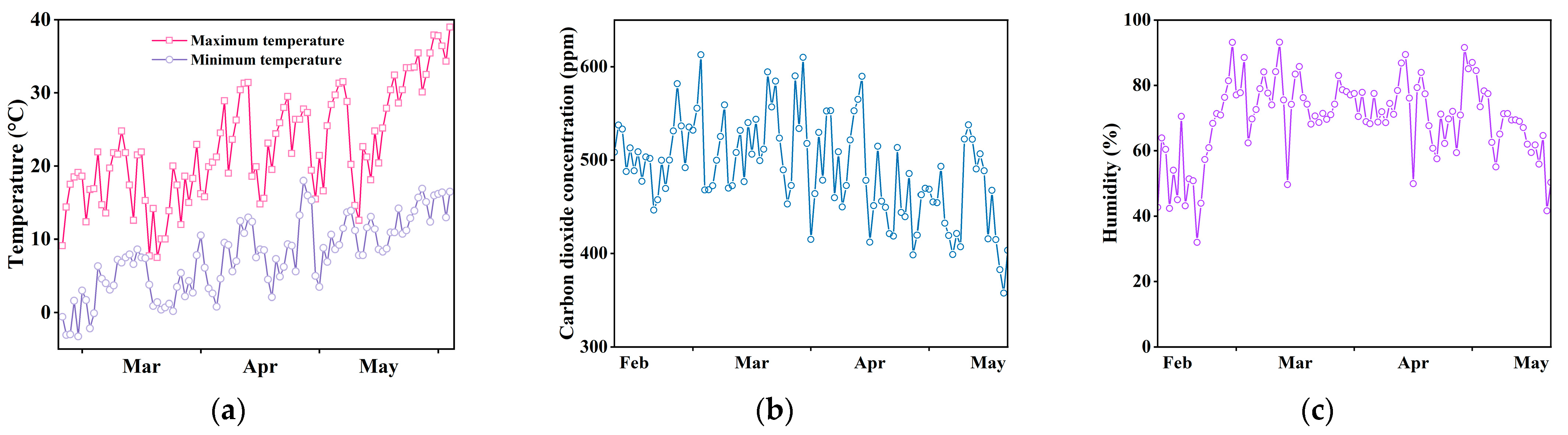
2.1. Site Description and Experimental Design

The experiment was set-up at Xinxiang, Henan, China (Figure 1) (113° 45′ 40′′ E, 35° 8′ 10′′ N). The area is located in two major basins, the Yellow River and the Haihe River, with fertile soil and a warm temperate continental monsoon climate. The experimental site was set-up with 6 different treatments of N fertilization. Ten winter wheat varieties were used, with 3 replicates for each treatment. All varieties were sown on 27 October 2021, with a plot size of 1.4 × 4 m and adjacent plots spaced 0.4 m apart from left to right and 1 m apart from front to back. Figure 2 shows the weather conditions recorded through small weather stations (Figure 1d) for the main growing season of winter wheat in 2022. The sprinkler irrigation of the test field used a lateral move sprinkler irrigation system (Figure 1d). The application of N fertilizer was carried out in 3 periods: regreening, jointing, and heading stages, and the amount of fertilizer in each period was divided by 1:1:1.

Table 1. The specific amount of nitrogen (N) fertilizer applied to each treatment.

N Fertilization Treatment	N1	N2	N3	N4	N5	N6
N fertilizer dosage	300 kg/hm2	240 kg/hm2	180 kg/hm2	120 kg/hm2	60 kg/hm2	0 kg/hm2

shows the amount of fertilizer applied for each treatment.

2.2. Data Acquisition

2.2.1. Field Data Acquisition

Six plants were randomly cut in each winter wheat plot on 11 April, 20 April, and 6 May 2022. All samples were then heated in an oven at 85 °C for 72 h to obtain dry matter. The dry material was crushed and sieved, 0.15 g was weighed into the decoction tube, 5 mL of concentrated sulfuric acid overnight was added, it was then decocted in a decoction oven and decocted in batches with hydrogen peroxide until the decoction solution was clarified, it was cooled, all was transferred to a 100 mL volumetric flask and placed overnight, and the supernatant was taken to measure the N content with a SEAL AA3 flow analyzer. The statistics of N content measurement results are shown in

Table 2. Descriptive statistics of N content in winter wheat.

Date	Sample Size	Max. (mg/g)	Min. (mg/g)	Mean (mg/g)	SD (mg/g)	CV (%)
11 April	180	33.048	11.715	22.11	4.918	22.242
20 April	180	27.234	9.124	16.68	4.174	25.025
6 May	180	23.964	7.431	14.11	3.711	26.301

SD: standard deviation; CV: coefficient of variation; mg/g: milligram per gram.

.

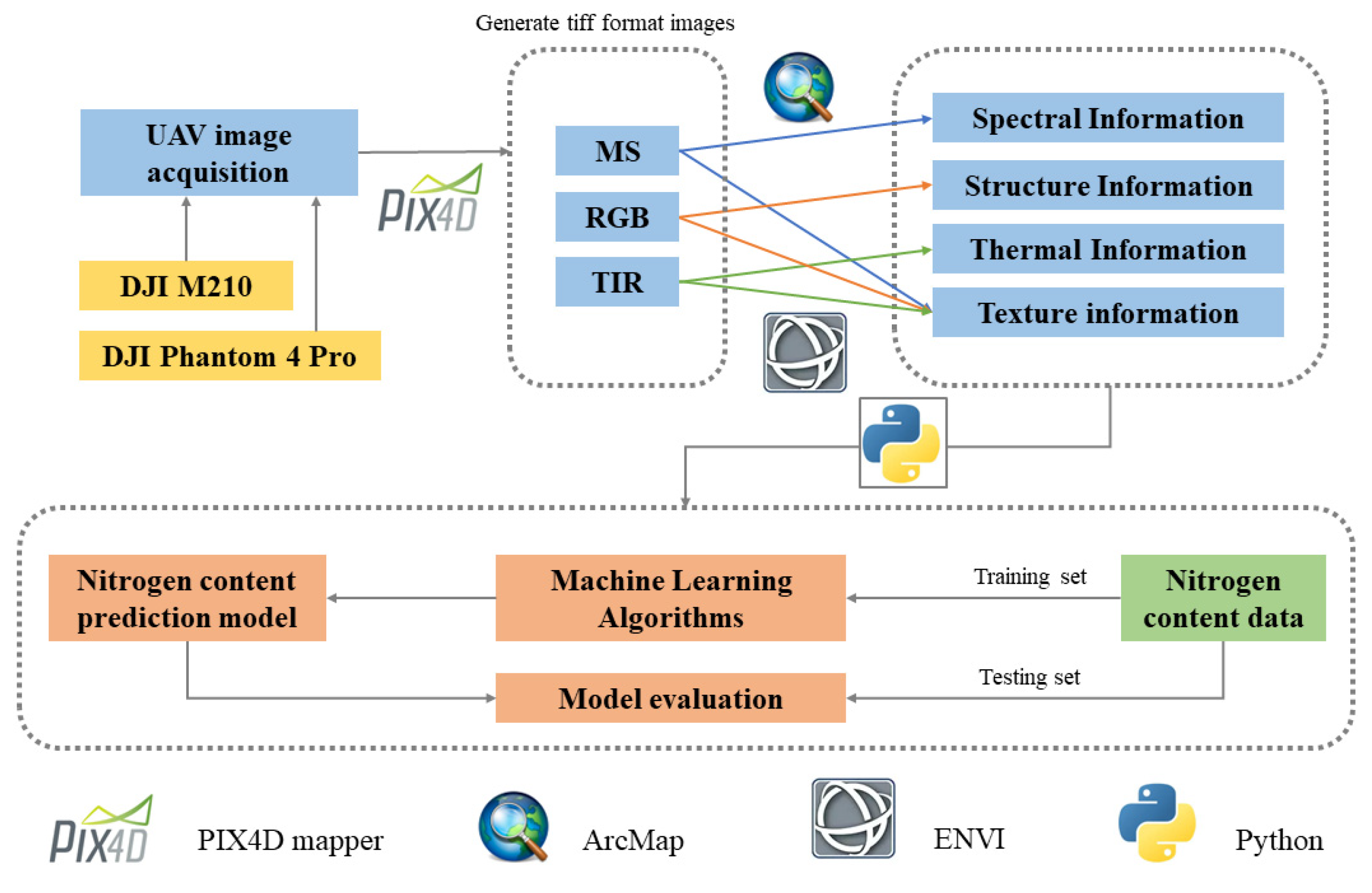
2.2.2. UAV Data Acquisition

In this experiment, MS and TIR data were collected using an M210 UAV (SZ DJI Technology Co., Shenzhen, China) fitted with the Red-Edge MX MS camera (MicaSense Inc., Shenzhen, China) and Zenmuse XT2 camera (SZ DJI Technology Co., Shenzhen, China). RGB data were collected using a digital camera equipped with the Phantom 4 Pro UAV (SZ DJI Technology Co., Shenzhen, China) (Figure 3).

The MS sensor includes five bands including red, green, blue, red-edge, and near-infrared with a resolution of 1280 × 960 pixels. The spatial resolution is 2 cm at a flight altitude of 30 m. The bandwidth is 10 nm for the red and red-edge bands, 20 nm for the blue and green bands, and 40 nm for the NIR. During shooting, the MS sensor automatically adjusts the exposure according to the ambient light, thus increasing the accuracy of the image [29]. The MS camera needs to take pictures of the radiation calibration plate before each takeoff and after each landing for radiation calibration operations during image stitching. The TIR sensor collects temperature information in the range of 7.5~13.5 μm with a resolution of 640 × 512 pixels. The spatial resolution is 3.9 cm at a flight altitude of 30 m. The RGB sensor has a resolution of 4000 × 3000 pixels and a spatial resolution of 0.8 cm at a flight altitude of 30 m.

The UAV images were obtained from 11:00 am to 1:00 PM on the same day (12 April 2022) after the on-site data collection, during which the light was sufficient and stable. The DJI ground station software allows users to plan the mission flight path and conduct UAV flight operations using the automatic flight control system. The flight altitude of all UAVs is set to 30 m. For all cameras, the heading overlap ratio was set to 85% and the side-overlap ratio was set to 80%. To verify the universality and feasibility of CSC in different periods, RGB image data were collected on 11 April and 6 May in the same way.

2.2.3. Image Preprocessing

The process of data preprocessing is shown in Figure 4. MS, RGB, and TIR images were stitched together using Pix4D software (Pix4D, Lausanne, Switzerland) to generate orthophotos. The processing included importing GCPs to the images, geolocalization, alignment of the images, construction of dense point clouds, and calibration of radiometric information. Using ArcMap 10.8 software (Environmental Systems Research Institute, Inc., Redlands, CA, USA), 180 polygons were drawn to segment each cell and superimposed on each image to extract the average pixel value of each cell in the image as the corresponding feature. The edges of the cells were omitted when drawing the polygons corresponding to each cell to avoid edge effects on the experiment.

2.3. Multimodal UAV Information Extraction

2.3.1. Canopy Spectral Information

In this study, 15 vegetation indices were constructed using multispectral reflectance (

Table 3. Different features extracted by different sensors.

Sensor Type	Feature Type	Features	Formulation	References
MS	Sp	Green (G), Red (R), Red-edge (RE), Near-infrared (NIR)	The raw value of each band	/
		Normalized Difference Vegetation Index	NDVI = (NIR − R)/(NIR + R)	[30]
		Optimized soil-adjusted vegetation index	OSAVI = (NIR − R)/(NIR − R + L) × (L = 0.16)	[31]
		Soil-Adjusted Vegetation Index	SAVI = ((NIR − R)/(NIR + R + L)) × (1 + L) × L = 0.5	[32]
		Modified Soil-adjusted Vegetation Index	MSAVI = (2 × NIR + 1 − sqrt ((2 × NIR + 1)2 − 8 × (NIR– RED)))/2	[33]
		Green normalized difference vegetation index	GNDVI = (NIR − G)/(NIR + G)	[34]
		Ratio vegetation index	RVI = NIR/R	[35]
		Green chlorophyll index	GCI = (NIR/G) − 1	[36]
		Red-edge chlorophyll index	RECI = (NIR/RE) − 1	[36]
		Green-red vegetation index	GRVI = (G − R)/(G + R)	[37]
		Normalized difference red-edge	NDRE = (NIR − RE)/(NIR + RE)	[38]
		Normalized difference red-edge index	NDREI = (RE − G)/(RE + G)	[19]
		Simplified canopy chlorophyll content index	SCCCI = NDRE/NDVI	[39]
		The enhanced vegetation index	EVI = 2.5 × (NIR − R)/(1 + NIR − 2.4 × R)	[38]
		Two-band enhanced vegetation index	EVI2 = 2.5 × (NIR − R)/(NIR + 2.4 × R + 1)	[40]
		Wide-dynamic-range vegetation index	WDRVI = (a × NIR − R)/(a × NIR + R)(a = 0.12)	[40]
	St	Vegetation fraction	FVC = Plant Pixels in Plot/Total Plot Pixels	[12]
RGB	St	canopy shade coverage	CSC = Shadow Pixels in Plot/Total Plot Pixels	/
TIR	Th	Normalized relative canopy temperature index	NRCT = (T − Tmin)/(Tmax − Tmin)	[26]
MS + RGB + TIR	Te	Gray-level co-occurrence matrix (GLCM)	ME, VA, DI, CON, HO, SE, COR, EN	[12]

Sp denotes spectral features, St denotes structural features, Th denotes thermal features, and Te denotes texture features.

). The five multispectral bands and the 15 vegetation indices were used as spectral information of the canopy.

2.3.2. Canopy Structure Information

In this study, the fractional vegetation cover (FVC) of winter wheat was calculated as canopy structure information, which represents the growth density of the crop and has a direct relationship with the crop growth condition [41]. The red-edge band in the multispectrum is sensitive to vegetation chlorophyll content and can effectively distinguish vegetation from bare soil in the map [42,43]; therefore, RE images were used to segment vegetation and soil to obtain FVC. There are many methods for FVC extraction, such as the threshold dichotomy method [44], the exponential time series graph intersection method [45,46], and the sample statistics method [47]. As the vegetation index histogram did not have a bimodal nature, due to the high winter wheat cover in this experimental plot, this study used the idea of the intersection point method of the index time series plot to determine the segmentation threshold. The histogram of the area with high winter wheat cover was superimposed on the histogram of the area with low cover, the color scale value corresponding to the intersection point of the two histogram curves was used as the initial segmentation threshold, and then the value obtained was slightly modified by the visual discrimination method to ensure the accuracy of the segmentation. As can be seen from Figure 5, the segmentation results were more accurate. Finally, the pixels of the plant fraction extracted from each plot were divided by the total number of pixels in that plot to obtain the FVC [12]. The FVC calculation formula is as follows:

$$\mathrm{FVC}=\frac{\mathrm{Total}\mathrm{number}\mathrm{of}\mathrm{vegetation}\mathrm{pixels}\mathrm{in}\mathrm{the}\mathrm{image}}{\mathrm{Total}\mathrm{number}\mathrm{of}\mathrm{pixels}\mathrm{in}\mathrm{the}\mathrm{image}}$$

(1)

In addition, this paper proposed canopy shade coverage (CSC) as new canopy structure information. The saturation and brightness of the RGB image were increased until the shadowed part of the canopy could be well distinguished from the part that receives direct light. A number of winter wheat canopy images were randomly intercepted in the winter wheat plots in the image, and the histogram of the green channel of each image was observed. It was found that the number of the leftmost color scale (indicating the darkest part of the image brightness) of the histogram of the green channel would increase significantly to form a half-peak, and the value of the color scale at the junction with the curve of the green channel of the original histogram was taken, and the average value obtained for each image was used as the threshold value for segmenting shadows (Figure 6). After thresholding the green channel of the RGB image, the CSC was obtained by dividing the number of pixels shaded in each cell by the total number of pixels in the cell. The CSC calculation formula is as follows:

$$\mathrm{CSC}=\frac{\mathrm{Total}\mathrm{number}\mathrm{of}\mathrm{shaded}\mathrm{pixels}\mathrm{in}\mathrm{the}\mathrm{graph}}{\mathrm{Total}\mathrm{number}\mathrm{of}\mathrm{pixels}\mathrm{in}\mathrm{the}\mathrm{graph}}$$

(2)

2.3.3. Canopy Thermal Information

Normalized relative canopy temperature (NRCT) [26,48] was calculated using the UAV TIR image:

$$\mathrm{NRCT}=\frac{\mathrm{T}-{\mathrm{T}}_{\min }}{{\mathrm{T}}_{\max }-{\mathrm{T}}_{\min }}$$

(3)

where T is the canopy temperature, T_max is the maximum temperature measured in all winter wheat plots, and T_min is the minimum temperature measured in all winter wheat plots. All units are in degrees Celsius.

2.3.4. Texture Features

The texture features of the R, G, red-edge, and NIR bands of MS as well as the grayscale map of RGB and TIR images were extracted using the grayscale co-generation matrix (GLCM) [49]. Eight GLCM-based texture features were derived, including the mean (ME), variance (VA), dissimilarity (DI), contrast (CON), homogeneity (HO), second-order moments (SE), correlation (COR), and entropy (EN) [50].

2.4. Machine Learning Methods

Three widely used machine learning methods were employed to construct relationships between multi-source remote sensing data and N content. The idea of Random Forest regression (RFR) [51] is ensemble learning, which is a branch of machine learning. It is composed of multiple trees, and its basic unit is the decision tree. In the training process, samples are randomly selected from the training set, repeated many times, and multiple decision trees are generated. For each decision tree, the results are predicted by passing random variables, to obtain a variety of results. The average value of these results is calculated to obtain the final prediction result of random forest regression. RFR reduces the risk of overfitting by averaging the prediction results of decision trees and is less affected by noise. Support vector regression (SVR) [52] is developed from the concept of support vector machines, and its core idea is to divide the points in the input variable space by categories. For inseparable space data samples, a low-dimensional linear inseparable space needs to be transformed into a high-dimensional linear separable space. Using the optimal sum function, the regression is achieved by constructing the hyperplane with the minimum distance from all sample points in the high-dimensional space. In this paper, we used both linear kernel functions, polynomial kernel functions, and radial basis kernel functions and selected the optimal results. The partial least squares regression (PLSR) [53] algorithm combines the advantages of multiple linear regression analysis, typical correlation analysis, and principal component analysis to find a linear regression model by projecting the predictor variables and the observed variables into a new space. The PLSR algorithm has the feature of being able to regress well even if the independent variables have multicollinearity.

During the modeling process, 3/4 of the data were randomly selected as the training set and the remaining 1/4 as the validation set. The mean absolute error (MAE) and the relative root-mean-square error (rRMSE) of the validation set were used to evaluate the model performance. Smaller values of MAE and rRMSE indicate the better prediction effect of the model. Pearson’s correlation coefficient (r) and coefficient of determination (R²) were also used in this paper, and higher r and R² indicate a higher correlation between them. The expressions are as follows:

$$\mathrm{MAE}=\frac{1}{\mathrm{n}}{\displaystyle \sum }_{\mathrm{i}=\mathrm{n}}^{\mathrm{n}}\left|{\mathrm{y}}_{\mathrm{i}}-{\hat{\mathrm{y}}}_{\mathrm{i}}\right|$$

(4)

$$\mathrm{rRMSE}=\frac{\sqrt{{{\displaystyle \sum }}_{\mathrm{i}=1}^{\mathrm{n}}{\left({\mathrm{y}}_{\mathrm{i}}-{\hat{\mathrm{y}}}_{\mathrm{i}}\right)}^2/\mathrm{n}}}{\overline{\mathrm{y}}}$$

(5)

$$\mathrm{r}=\frac{{{\displaystyle \sum }}_{\mathrm{i}=1}^{\mathrm{n}}\left({\mathrm{x}}_{\mathrm{i}}-\overline{\mathrm{x}}\right)\left({\mathrm{y}}_{\mathrm{i}}-\overline{\mathrm{y}}\right)}{\sqrt{{{\displaystyle \sum }}_{\mathrm{i}=1}^{\mathrm{n}}{\left({\mathrm{x}}_{\mathrm{i}}-\overline{\mathrm{x}}\right)}^2}\sqrt{{{\displaystyle \sum }}_{\mathrm{i}=1}^{\mathrm{n}}{\left({\mathrm{y}}_{\mathrm{i}}-\overline{\mathrm{y}}\right)}^2}}$$

(6)

$${\mathrm{R}}^2=1-\frac{{{\displaystyle \sum }}_{\mathrm{i}=1}^{\mathrm{n}}{\left({\hat{\mathrm{y}}}_{\mathrm{i}}-{\mathrm{y}}_{\mathrm{i}}\right)}^2}{{{\displaystyle \sum }}_{\mathrm{i}=1}^{\mathrm{n}}{\left({\mathrm{y}}_{\mathrm{i}}-\overline{\mathrm{y}}\right)}^2}$$

(7)

where n is the total number of samples in the test set. ${\mathrm{x}}_{\mathrm{i}}$ and $\overline{\mathrm{x}}$ are the variables x and measurement of x, respectively. ${\mathrm{y}}_{\mathrm{i}}$ and ${\hat{\mathrm{y}}}_{\mathrm{i}}$ are the measured and predicted values of N content, respectively. $\overline{\mathrm{y}}$ is the mean value of the measured values of N content.

3. Results

3.1. Relationship between CSC and N Content of Winter Wheat

The scatter plot of winter wheat and CSC is shown in Figure 7, which showed a significant correlation, r of 0.677, R² of 0.459, and a p-value less than 0.01, with a highly significant difference. The CSC increased slowly or even ceased to increase when the N content reached above 22, which might be the saturation of the CSC. As canopy leaf shadow coverage and plant coverage are the same structural features obtained by thresholding the UAV images, there is a possibility of covariance, so covariance analysis was performed for both. The variance inflation factor (VIF) of both was 7.937, which is less than 10, and there was no collinearity between them. This indicates that the canopy leaf shadow coverage can be used as an input feature to predict the N content of winter wheat.

In order to eliminate the contingency of the correlation between CSC in a single period and N content in winter wheat, the correlation analysis between CSC and N content in multiple periods was carried out. As shown in Figure 8, the r of CSC and N content in several periods were greater than 0.4 and were significantly correlated. This conclusion verified the applicability of CSC over multiple fertility periods, and to a certain extent, it eliminated the possibility that the correlation between CSC and N content was contingent.

3.2. Estimation of N Content under a Single Data Source

The accuracy of the RFR, SVR, and PLSR in estimating wheat N content using individual sensor data is summarized in

Table 4. Accuracy of predicting N content in winter wheat using single-source sensors.

Sensor Type	Feature Type	Metrics	RFR	SVR	PLSR
MS	sp	MAE (mg/g)	1.837	2.193	2.197
		rRMSE%	13.649	16.894	16.266
	sp + te	MAE (mg/g)	1.791	1.805	1.841
		rRMSE%	13.151	14.059	13.435
RGB	st	MAE (mg/g)	2.044	2.379	2.29
		rRMSE%	14.324	17.657	16.823
	st + te	MAE (mg/g)	1.724	1.93	1.882
		rRMSE%	12.51	13.753	13.323
TIR	th	MAE (mg/g)	3.479	2.972	3.643
		rRMSE%	25.49	21.062	26.625
	th + te	MAE (mg/g)	1.939	2.098	2.266
		rRMSE%	15.617	15.136	16.472

. The MAE of the N content prediction model for the spectral information obtained from the MS sensor ranged from 1.837 mg/g to 2.193 mg/g. The accuracy of the models obtained using MS was better than those of RGB and TIR, regardless of which algorithm was used. The performance of the canopy structure information obtained from the RGB sensor was slightly lower than that of the spectral information based on the MS sensor. After adding texture features at the same time, the accuracy of the model obtained by the RGB data was comparable to that of the MS data. The thermal information was the worst predictor of N content. However, when using two feature categories (th and te), the MAE range of the model was reduced from 2.972~3.643 mg/g to 1.939~2.266 mg/g, and the rRMSE range was reduced from 21.062~26.625% to 15.136~16.472%.

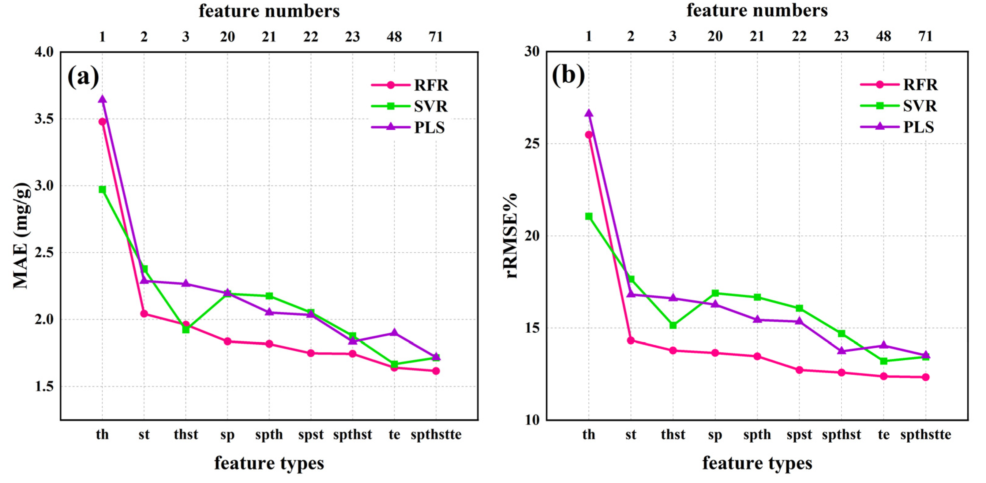
3.3. N Content Estimation by Fusing Multiple-Source Data

To explore the influence of multi-source data fusion on the accuracy of the N content prediction model, the UAV data were combined according to different feature types, as shown in

Table 5. Accuracy of using multi-source sensors to predict N content in winter wheat.

Sensor Type	Feature Type	Number of Features	Metrics	RFR	SVR	PLSR
MS + RGB	sp st	22	MAE (mg/g)	1.749	2.053	2.035
			rRMSE%	12.725	16.074	15.345
MS + TIR	sp th	21	MAE (mg/g)	1.818	2.177	2.053
			rRMSE%	13.465	16.675	15.442
RGB + TIR	st th	3	MAE (mg/g)	1.962	1.923	2.268
			rRMSE%	13.778	15.147	16.608
MS + RGB + TIR	sp st th	23	MAE (mg/g)	1.745	1.878	1.835
			rRMSE%	12.584	14.698	13.735
MS + RGB + TIR	te	48	MAE (mg/g)	1.641	1.667	1.899
			rRMSE%	12.377	13.205	14.049
MS + RGB + TIR	sp st th te	71	MAE (mg/g)	1.616	1.715	1.718
			rRMSE%	12.333	13.432	13.519

. For the prediction of the N content by combining dual sensors, the three models constructed by combining MS and RGB had the best prediction results, with MAE ranging from 1.749 mg/g to 2.053 mg/g and rRMSE ranging from 12.725% to 16.074%, which had an enhancement effect relative to the prediction model constructed by using only MS sensors. No matter which modeling method was used, the prediction effect of the canopy spectral, structural, and thermal information fusion of MS, RGB, and TIR sensors was significantly improved compared with the fusion of any two sensors, with MAE ranging from 1.745 mg/g to 1.878 mg/g and rRMSE ranging from 12.584% to 14.698%. After the canopy texture features of the MS, RGB, and TIR sensors were fused, the accuracy of the N content prediction model was similar to that obtained by the fusion of the spectral, structural, and thermal information of the three sensors. After the canopy spectral, structural, thermal, and texture information was fused, the accuracy of the N content prediction model was further improved. The MAE was from 1.616 mg/g to 1.718 mg/g, and the rRMSE was from 12.333% to 13.519%, but the improvement effect was small.

The comparison of the performance for the three machine learning algorithms is shown in Figure 9. RFR generally showed a higher accuracy than SVR and PLSR, and achieved the highest accuracy in fusing canopy spectral, structural, thermal, and textural information from MS, RGB, and TIR with an MAE of 1.616 mg/g and rRMSE of 12.333%. However, the advantages of RFR were not obvious when there were only single input features. With the increase in the type and number of input features, the MAE and rRMSE of all methods decreased gradually, which indicated that multi-source data fusion could improve the prediction accuracy of N content in winter wheat. The scatter plot of the predicted and measured values of the best model for each algorithm is shown in Figure 10. The distributions of the scatter plots for SVR and PLSR were very similar, with the best fit of the predicted values to the measured values for RFR. When the measured value of N content reached above 23, the predicted value increased slowly with the increase in the measured value and reached slight saturation.

4. Discussion

4.1. Relationship between Drone Images and N Levels

In this experiment, three sensors, MS, RGB, and TIR, are used to predict N content in winter wheat. MS is the most sensitive sensor for N content, and because it contains 5 bands, it can provide more information about the growth status of crops. R and G bands can reflect the growth of the crop canopy to a certain extent [8], and red-edge and NIR are more sensitive to crop structure and chlorophyll level [43,54]. However, RGB and TIR contain relatively few bands. In particular, TIR only provides the temperature information of the canopy, and the information that can be extracted is limited, so the prediction effect of N content is not as good as those of MS and RGB. However, after the previous research and this paper, there is a certain correlation between the thermal information and the N content [55,56]. The fusion of TIR with other sensors can improve the accuracy of the model [27], indicating that TIR still has a certain value in predicting N content.

The fusion of MS, RGB, and TIR sensors can improve the prediction effect of N content, which is consistent with the previous research results [27]. One of the reasons is that there is a complementary relationship between different types of features extracted by different sensors [12]. The spectral information and vegetation index provided by MS are effective indicators for monitoring and predicting crop growth and traits, and a large number of studies in the literature support this view [4,57,58,59,60]. Canopy structure information is an effective variable for predicting crop phenotypes. The plant coverage used in this study has been proven to be an effective indicator for predicting N content in winter wheat. Crop canopy temperature is related to crop photosynthesis, crop growth status, and chlorophyll content, which determine the strength of photosynthesis, and N content has a decisive effect on both [61,62], so N content will inevitably affect crop canopy temperature [63].

In this study, when the measured value of N content reaches more than 20 mg/g, the predicted value increases slowly with the increase in the measured value and reaches light saturation [12]. At this time, the reflectance of the UAV spectral image no longer changes significantly with the increase in N content (Figure 9). RFR is less affected by light saturation than the other two machine learning models, which indicates that it can process peak information to a certain extent.

4.2. Relationship between CSC and N Content

The CSC proposed in this paper is rarely used in crop phenotypic prediction, and most of the previous studies are aimed at eliminating shadows [64,65]. Leaf shadow coverage may be related to the number and size of canopy leaves and canopy leaf structure, and in general, the higher the number of crop leaves, the denser the shadow. CSC and N content predictions are the same at N contents greater than 20 mg/g. The saturation phenomenon, such as the data points in the blue circle in Figure 6, may be due to the change in canopy leaf size and number with the increase in N content, reaching saturation and making it difficult to have a great breakthrough. The CSC is also related to the solar altitude angle; the smaller the solar angle, the larger the shadow area produced by the blade, which, in turn, will lead to a larger CSC as well. More research is needed to verify whether the saturation of CSC is inevitable. In this study, only noon images were used, when the solar altitude angle was close to 90°, which produced less leaf shadow. The relationship between the CSC and N content of winter wheat at other solar altitude angles is not considered. It is necessary to study the relationship between CSC and different traits of other crops at different solar altitude angles in follow-up work. Because of the significant correlation between CSC and N content, canopy leaf cover can be added to the inversion work of phenotypic information of different crops in subsequent studies. It is necessary to further refine the method of extracting leaf shadow cover.

4.3. Limitations and Implications of the Study

This study fuses three sensor image data sources and achieves a good improvement in predicting the N content of winter wheat relative to the single-sensor model. However, the information that these sensors can provide is limited, and hyperspectral and LIDAR data can be added to this study in the next step to reduce the redundancy of data and increase the type of data, as well as the stability of the model. The CSC proposed in this paper can be used as a new input feature for inverse prediction of N content in winter wheat, which is also well validated in this paper. The CSC as a structural feature is different from the extraction method of features such as FVC and plant height commonly used by previous authors, so it can be used as an input feature together with data from multiple sensors to increase the diversity of data. However, at the late stage of winter wheat fertility, when the leaves of plants with different N contents have all reached complete canopy coverage, it results in relatively insignificant differences in CSC between small zones. This is well supported by the low Pearson correlation coefficient between CSC and N content on 6 May in Figure 8.

5. Conclusions

The predictive effect of multi-source data fusion on the N content of winter wheat was investigated by using machine learning algorithms. The main conclusions of this paper are as follows:

1. MS outperformed RGB and TIR in predicting N content in winter wheat in a single-sensor-based model for predicting N content. Although TIR was less effective, it also showed potential in the prediction of N content in winter wheat.

2. No matter which machine learning algorithm was used, the prediction effect of multi-source data fusion on the N content of winter wheat had a certain improvement effect compared with a single sensor.

3. Whether using multiple sensors or only a single sensor, the random forest algorithm showed a better accuracy than support vector machines and least squares.

4. CSC can be used as an effective structural feature to predict the N content of winter wheat.

The purpose of this study was to improve the accuracy of predicting the N content of winter wheat, which is important for specifying a reasonable nitrogen fertilizer application schedule and a further yield prediction at the early stage of winter wheat fertility.

References

1. Lin, M.Y.; Lynch, V.; Ma, D.D.; Maki, H.; Jin, J.; Tuinstra, M. Multi-Species Prediction of Physiological Traits with Hyperspectral Modeling. Plants 2022, 11, 15. [Google Scholar] [CrossRef] [PubMed]
2. Wang, Z.L.; Chen, J.X.; Zhang, J.W.; Fan, Y.F.; Cheng, Y.J.; Wang, B.B.; Wu, X.L.; Tan, X.M.; Tan, T.T.; Li, S.L.; et al. Predicting grain yield and protein content using canopy reflectance in maize grown under different water and nitrogen levels. Field Crops Res. 2021, 260, 15. [Google Scholar] [CrossRef]
3. Calderon, R.; Rajendiran, K.; Kim, U.J.; Palma, P.; Arancibia-Miranda, N.; Silva-Moreno, E.; Corradini, F. Sources and fates of perchlorate in soils in Chile: A case study of perchlorate dynamics in soil-crop systems using lettuce (Lactuca sativa) fields. Environ. Pollut. 2020, 264, 7. [Google Scholar] [CrossRef] [PubMed]
4. Osco, L.P.; Ramos, A.P.M.; Pereira, D.R.; Moriya, E.A.S.; Imai, N.N.; Matsubara, E.T.; Estrabis, N.; de Souza, M.; Marcato, J.; Goncalves, W.N.; et al. Predicting Canopy Nitrogen Content in Citrus-Trees Using Random Forest Algorithm Associated to Spectral Vegetation Indices from UAV-Imagery. Remote Sens. 2019, 11, 2925. [Google Scholar] [CrossRef] [Green Version]
5. Goffart, D.; Ben Abdallah, F.; Curnel, Y.; Planchon, V.; Defourny, P.; Goffart, J.P. In-Season Potato Crop Nitrogen Status Assessment from Satellite and Meteorological Data. Potato Res. 2022, 65, 729–755. [Google Scholar] [CrossRef]
6. Bossung, C.; Schlerf, M.; Machwitz, M. Estimation of canopy nitrogen content in winter wheat from Sentinel-2 images for operational agricultural monitoring. Precis. Agric. 2022, 1–24. [Google Scholar] [CrossRef]
7. Iatrou, M.; Karydas, C.; Iatrou, G.; Pitsiorlas, I.; Aschonitis, V.; Raptis, I.; Mpetas, S.; Kravvas, K.; Mourelatos, S. Topdressing Nitrogen Demand Prediction in Rice Crop Using Machine Learning Systems. Agriculture 2021, 11, 312. [Google Scholar] [CrossRef]
8. Berger, K.; Verrelst, J.; Feret, J.B.; Hank, T.; Wocher, M.; Mauser, W.; Camps-Valls, G. Retrieval of aboveground crop nitrogen content with a hybrid machine learning method. Int. J. Appl. Earth Obs. Geoinf. 2020, 92, 15. [Google Scholar] [CrossRef]
9. Yu, D.Y.; Zha, Y.Y.; Sun, Z.G.; Li, J.; Jin, X.L.; Zhu, W.X.; Bian, J.; Ma, L.; Zeng, Y.J.; Su, Z.B. Deep convolutional neural networks for estimating maize above-ground biomass using multi-source UAV images: A comparison with traditional machine learning algorithms. Precis. Agric. 2022, 1–22. [Google Scholar] [CrossRef]
10. Revill, A.; Florence, A.; MacArthur, A.; Hoad, S.; Rees, R.; Williams, M. Quantifying Uncertainty and Bridging the Scaling Gap in the Retrieval of Leaf Area Index by Coupling Sentinel-2 and UAV Observations. Remote Sens. 2020, 12, 1843. [Google Scholar] [CrossRef]
11. Hasan, U.; Sawut, M.; Chen, S.S. Estimating the Leaf Area Index of Winter Wheat Based on Unmanned Aerial Vehicle RGB-Image Parameters. Sustainability 2019, 11, 6829. [Google Scholar] [CrossRef] [Green Version]
12. Maimaitijiang, M.; Sagan, V.; Sidike, P.; Hartling, S.; Esposito, F.; Fritschi, F.B. Soybean yield prediction from UAV using multimodal data fusion and deep learning. Remote Sens. Environ. 2020, 237, 20. [Google Scholar] [CrossRef]
13. Fu, Z.P.; Jiang, J.; Gao, Y.; Krienke, B.; Wang, M.; Zhong, K.T.; Cao, Q.; Tian, Y.C.; Zhu, Y.; Cao, W.X.; et al. Wheat Growth Monitoring and Yield Estimation based on Multi-Rotor Unmanned Aerial Vehicle. Remote Sens. 2020, 12, 508. [Google Scholar] [CrossRef] [Green Version]
14. Berger, K.; Verrelst, J.; Feret, J.B.; Wang, Z.H.; Wocher, M.; Strathmann, M.; Danner, M.; Mauser, W.; Hank, T. Crop nitrogen monitoring: Recent progress and principal developments in the context of imaging spectroscopy missions. Remote Sens. Environ. 2020, 242, 18. [Google Scholar] [CrossRef] [PubMed]
15. Han, W.; Tang, J.; Zhang, L.; Niu, Y.; Wang, T. Maize Water Use Efficiency and Biomass Estimation Based on Unmanned Aerial Vehicle Remote Sensing. Trans. Chin. Soc. Agric. Mach. 2021, 52, 129–141. [Google Scholar]
16. Li, C.C.; Cui, Y.Q.; Ma, C.Y.; Niu, Q.L.; Li, J.B. Hyperspectral inversion of maize biomass coupled with plant height data. Crop Sci. 2021, 61, 2067–2079. [Google Scholar] [CrossRef]
17. Tao, H.; Xu, L.; Feng, H.; Yang, G.; Dai, Y.; Niu, Y. Estimation of Plant Height and Leaf Area Index of Winter Wheat Based on UAV Hyperspectral Remote Sensing. Trans. Chin. Soc. Agric. Mach. 2020, 51, 193–201. [Google Scholar]
18. Zhang, X.W.; Zhang, K.F.; Sun, Y.Q.; Zhao, Y.D.; Zhuang, H.F.; Ban, W.; Chen, Y.; Fu, E.R.; Chen, S.; Liu, J.X.; et al. Combining Spectral and Texture Features of UAS-Based Multispectral Images for Maize Leaf Area Index Estimation. Remote Sens. 2022, 14, 331. [Google Scholar] [CrossRef]
19. Hassan, M.A.; Yang, M.J.; Rasheed, A.; Jin, X.L.; Xia, X.C.; Xiao, Y.G.; He, Z.H. Time-Series Multispectral Indices from Unmanned Aerial Vehicle Imagery Reveal Senescence Rate in Bread Wheat. Remote Sens. 2018, 10, 809. [Google Scholar] [CrossRef] [Green Version]
20. Panek, E.; Gozdowski, D.; Stepien, M.; Samborski, S.; Rucinski, D.; Buszke, B. Within-Field Relationships between Satellite-Derived Vegetation Indices, Grain Yield and Spike Number of Winter Wheat and Triticale. Agronomy 2020, 10, 1842. [Google Scholar] [CrossRef]
21. Yang, B.H.; Zhu, Y.; Zhou, S.J. Accurate Wheat Lodging Extraction from Multi-Channel UAV Images Using a Lightweight Network Model. Sensors 2021, 21, 16. [Google Scholar] [CrossRef]
22. Walter, J.D.C.; Edwards, J.; McDonald, G.; Kuchel, H. Estimating Biomass and Canopy Height with LiDAR for Field Crop Breeding. Front. Plant Sci. 2019, 10, 16. [Google Scholar] [CrossRef] [PubMed] [Green Version]
23. Gilliot, J.M.; Michelin, J.; Hadjard, D.; Houot, S. An accurate method for predicting spatial variability of maize yield from UAV-based plant height estimation: A tool for monitoring agronomic field experiments. Precis. Agric. 2021, 22, 897–921. [Google Scholar] [CrossRef]
24. Wang, Y.; Fang, H.L. Estimation of LAI with the LiDAR Technology: A Review. Remote Sens. 2020, 12, 3457. [Google Scholar] [CrossRef]
25. Shendryk, Y.; Sofonia, J.; Garrard, R.; Rist, Y.; Skocaj, D.; Thorburn, P. Fine-scale prediction of biomass and leaf nitrogen content in sugarcane using UAV LiDAR and multispectral imaging. Int. J. Appl. Earth Obs. Geoinf. 2020, 92, 14. [Google Scholar] [CrossRef]
26. Elsayed, S.; Elhoweity, M.; Ibrahim, H.H.; Dewir, Y.H.; Migdadi, H.M.; Schmidhalter, U. Thermal imaging and passive reflectance sensing to estimate the water status and grain yield of wheat under different irrigation regimes. Agric. Water Manag. 2017, 189, 98–110. [Google Scholar] [CrossRef]
27. Pancorbo, J.L.; Camino, C.; Alonso-Ayuso, M.; Raya-Sereno, M.D.; Gonzalez-Fernandez, I.; Gabriel, J.L.; Zarco-Tejada, P.J.; Quemada, M. Simultaneous assessment of nitrogen and water status in winter wheat using hyperspectral and thermal sensors. Eur. J. Agron. 2021, 127, 14. [Google Scholar] [CrossRef]
28. Fu, Y.Y.; Yang, G.J.; Song, X.Y.; Li, Z.H.; Xu, X.G.; Feng, H.K.; Zhao, C.J. Improved Estimation of Winter Wheat Aboveground Biomass Using Multiscale Textures Extracted from UAV-Based Digital Images and Hyperspectral Feature Analysis. Remote Sens. 2021, 13, 581. [Google Scholar] [CrossRef]
29. Fei, S.P.; Hassan, M.A.; Xiao, Y.G.; Su, X.; Chen, Z.; Cheng, Q.; Duan, F.Y.; Chen, R.Q.; Ma, Y.T. UAV-based multi-sensor data fusion and machine learning algorithm for yield prediction in wheat. Precis. Agric. 2022, 26. [Google Scholar] [CrossRef]
30. Tucker, C.J. Red and photographic infrared linear combinations for monitoring vegetation. Remote Sens. Environ. 1979, 8, 127–150. [Google Scholar] [CrossRef] [Green Version]
31. Steven, M.D. The sensitivity of the OSAVI vegetation index to observational parameters. Remote Sens. Environ. 1998, 63, 49–60. [Google Scholar] [CrossRef]
32. Hatfield, J.L.; Prueger, J.H. Value of Using Different Vegetative Indices to Quantify Agricultural Crop Characteristics at Different Growth Stages under Varying Management Practices. Remote Sens. 2010, 2, 562–578. [Google Scholar] [CrossRef]
33. Qi, J.; Chehbouni, A.; Huete, A.R.; Kerr, Y.H.; Sorooshian, S. A modified soil adjusted vegetation index. Remote Sens. Environ. 1994, 48, 119–126. [Google Scholar] [CrossRef]
34. Candiago, S.; Remondino, F.; De Giglio, M.; Dubbini, M.; Gattelli, M. Evaluating Multispectral Images and Vegetation Indices for Precision Farming Applications from UAV Images. Remote Sens. 2015, 7, 4026–4047. [Google Scholar] [CrossRef] [Green Version]
35. Broge, N.H.; Mortensen, J.V. Deriving green crop area index and canopy chlorophyll density of winter wheat from spectral reflectance data. Remote Sens. Environ. 2002, 81, 45–57. [Google Scholar] [CrossRef]
36. Gitelson, A.A.; Vina, A.; Ciganda, V.; Rundquist, D.C.; Arkebauer, T.J. Remote estimation of canopy chlorophyll content in crops. Geophys. Res. Lett. 2005, 32, 4. [Google Scholar] [CrossRef] [Green Version]
37. Bendig, J.; Yu, K.; Aasen, H.; Bolten, A.; Bennertz, S.; Broscheit, J.; Gnyp, M.L.; Bareth, G. Combining UAV-based plant height from crop surface models, visible, and near infrared vegetation indices for biomass monitoring in barley. Int. J. Appl. Earth Obs. Geoinf. 2015, 39, 79–87. [Google Scholar] [CrossRef]
38. Potgieter, A.B.; George-Jaeggli, B.; Chapman, S.C.; Laws, K.; Cadavid, L.A.S.; Wixted, J.; Watson, J.; Eldridge, M.; Jordan, D.R.; Hammer, G.L. Multi-Spectral Imaging from an Unmanned Aerial Vehicle Enables the Assessment of Seasonal Leaf Area Dynamics of Sorghum Breeding Lines. Front. Plant Sci. 2017, 8, 11. [Google Scholar] [CrossRef]
39. Ballester, C.; Hornbuckle, J.; Brinkhoff, J.; Smith, J.; Quayle, W. Assessment of In-Season Cotton Nitrogen Status and Lint Yield Prediction from Unmanned Aerial System Imagery. Remote Sens. 2017, 9, 1149. [Google Scholar] [CrossRef] [Green Version]
40. Dempewolf, J.; Adusei, B.; Becker-Reshef, I.; Hansen, M.; Potapov, P.; Khan, A.; Barker, B. Wheat Yield Forecasting for Punjab Province from Vegetation Index Time Series and Historic Crop Statistics. Remote Sens. 2014, 6, 9653–9675. [Google Scholar] [CrossRef] [Green Version]
41. Wu, H.; Cui, K.; Zhang, X.; Xue, X.; Zheng, W.; Wang, Y. Improving Accuracy of Fine Leaf Crop Coverage by Improved K-means Algorithm. Trans. Chin. Soc. Agric. Mach. 2019, 50, 42–50. [Google Scholar]
42. Qiao, L.; Tang, W.J.; Gao, D.H.; Zhao, R.M.; An, L.L.; Li, M.Z.; Sun, H.; Song, D. UAV-based chlorophyll content estimation by evaluating vegetation index responses under different crop coverages. Comput. Electron. Agric. 2022, 196, 12. [Google Scholar] [CrossRef]
43. Kang, Y.P.; Meng, Q.Y.; Liu, M.; Zou, Y.F.; Wang, X.M. Crop Classification Based on Red Edge Features Analysis of GF-6 WFV Data. Sensors 2021, 21, 4328. [Google Scholar] [CrossRef] [PubMed]
44. Shuai, S.; Zhang, Z.; Lyu, X.; Chen, S.; Ma, Z.; Xie, C. Remote sensing monitoring of vegetation phenological characteristics and vegetation health status in mine restoration areas. Trans. Chin. Soc. Agric. Eng. 2021, 37, 224–234. [Google Scholar]
45. Yin, L.; Zhou, Z.; Li, S.; Huang, D. Research on Vegetation Extraction and Fractional Vegetation Cover of Karst Area Based on Visible Light Image of UAV. Acta Agrestia Sin. 2020, 28, 1664–1672. [Google Scholar]
46. Li, B.; Liu, R.; Liu, S.; Liu, Q.; Liu, F.; Zhou, G. Monitoring vegetation coverage variation of winter wheat by low-altitude UAV remote sensing system. Trans. Chin. Soc. Agric. Eng. 2012, 28, 160–165. [Google Scholar]
47. Liu, Z.; Huang, J.; Wu, X.; Dong, Y.; Wang, F.; Liu, P. Hyperspectral remote sensing estimation models on vegetation coverage of natural grassland. Ying Yong Sheng Tai Xue Bao = J. Appl. Ecol. 2006, 17, 997–1002. [Google Scholar]
48. Elsayed, S.; Rischbeck, P.; Schmidhalter, U. Comparing the performance of active and passive reflectance sensors to assess the normalized relative canopy temperature and grain yield of drought-stressed barley cultivars. Field Crops Res. 2015, 177, 148–160. [Google Scholar] [CrossRef]
49. Haralick, R.M.; Shanmugam, K.S. Combined spectral and spatial processing of ERTS imagery data. Remote Sens. Environ. 1974, 3, 3–13. [Google Scholar] [CrossRef] [Green Version]
50. Nichol, J.E.; Sarker, M.L.R. Improved Biomass Estimation Using the Texture Parameters of Two High-Resolution Optical Sensors. IEEE Trans. Geosci. Remote Sens. 2011, 49, 930–948. [Google Scholar] [CrossRef] [Green Version]
51. Breiman, L. Random forests. Mach. Learn. 2001, 45, 5–32. [Google Scholar] [CrossRef] [Green Version]
52. Smola, A.J.; Scholkopf, B. A tutorial on support vector regression. Stat. Comput. 2004, 14, 199–222. [Google Scholar] [CrossRef] [Green Version]
53. Abdi, H. Partial least squares regression and projection on latent structure regression (PLS Regression). Wiley Interdiscip. Rev.-Comput. Stat. 2010, 2, 97–106. [Google Scholar] [CrossRef]
54. Hein, P.R.G.; Chaix, G. NIR spectral heritability: A promising tool for wood breeders? J. Near Infrared Spectrosc. 2014, 22, 141–147. [Google Scholar] [CrossRef]
55. Klem, K.; Zahora, J.; Zemek, F.; Trunda, P.; Tuma, I.; Novotna, K.; Hodanova, P.; Rapantova, B.; Hanus, J.; Vavrikova, J.; et al. Interactive effects of water deficit and nitrogen nutrition on winter wheat. Remote sensing methods for their detection. Agric. Water Manag. 2018, 210, 171–184. [Google Scholar] [CrossRef]
56. Masseroni, D.; Ortuani, B.; Corti, M.; Gallina, P.M.; Cocetta, G.; Ferrante, A.; Facchi, A. Assessing the Reliability of Thermal and Optical Imaging Techniques for Detecting Crop Water Status under Different Nitrogen Levels. Sustainability 2017, 9, 1548. [Google Scholar] [CrossRef] [Green Version]
57. Haboudane, D.; Miller, J.R.; Tremblay, N.; Zarco-Tejada, P.J.; Dextraze, L. Integrated narrow-band vegetation indices for prediction of crop chlorophyll content for application to precision agriculture. Remote Sens. Environ. 2002, 81, 416–426. [Google Scholar] [CrossRef]
58. Li, X.H.; Ba, Y.X.; Zhang, M.Q.; Nong, M.L.; Yang, C.; Zhang, S.M. Sugarcane Nitrogen Concentration and Irrigation Level Prediction Based on UAV Multispectral Imagery. Sensors 2022, 22, 2711. [Google Scholar] [CrossRef]
59. Bukowiecki, J.; Rose, T.; Ehlers, R.; Kage, H. High-Throughput Prediction of Whole Season Green Area Index in Winter Wheat With an Airborne Multispectral Sensor. Front. Plant Sci. 2020, 10, 14. [Google Scholar] [CrossRef]
60. White, C.M.; Bradley, B.; Finney, D.M.; Kaye, J.P. Predicting Cover Crop Nitrogen Content with a Handheld Normalized Difference Vegetation Index Meter. Agric. Environ. Lett. 2019, 4, 4. [Google Scholar] [CrossRef] [Green Version]
61. Hammad, H.M.; Abbas, F.; Ahmad, A.; Bakhat, H.F.; Farhad, W.; Wilkerson, C.J.; Fahad, S.; Hoogenboom, G. Predicting Kernel Growth of Maize under Controlled Water and Nitrogen Applications. Int. J. Plant Prod. 2020, 14, 609–620. [Google Scholar] [CrossRef]
62. Chen, Z.F.; Zhang, Y.; Yang, Y.Q.; Shi, X.R.; Zhang, L.; Jia, G.W. Hierarchical nitrogen-doped holey graphene as sensitive electrochemical sensor for methyl parathion detection. Sens. Actuator B-Chem. 2021, 336, 9. [Google Scholar] [CrossRef]
63. Safa, M.; Martin, K.E.; Kc, B.; Khadka, R.; Maxwell, T.M.R. Modelling nitrogen content of pasture herbage using thermal images and artificial neural networks. Therm. Sci. Eng. Prog. 2019, 11, 283–288. [Google Scholar] [CrossRef]
64. Bu, R.B.; Xiong, J.T.; Chen, S.M.; Zheng, Z.H.; Guo, W.T.; Yang, Z.G.; Lin, X.Y. A shadow detection and removal method for fruit recognition in natural environments. Precis. Agric. 2020, 21, 782–801. [Google Scholar] [CrossRef]
65. Wu, S.T.; Hsieh, Y.T.; Chen, C.T.; Chen, J.C. A Comparison of 4 Shadow Compensation Techniques for Land Cover Classification of Shaded Areas from High Radiometric Resolution Aerial Images. Can. J. Remote Sens. 2014, 40, 315–326. [Google Scholar] [CrossRef]
Figure 1. Test field located in Henan Province, China. (a) Overview of China, (b) overview of Henan Province, (c) trial field layout, and (d) field photos.
Agriculture 12 01752 g001
Figure 2. Changes in meteorological data for the main growing season of winter wheat in 2022. (a) Daily maximum and minimum temperatures, (b) daily average carbon dioxide concentration, and (c) average humidity in the test plots.
Agriculture 12 01752 g002
Figure 3. Unmanned aerial vehicles (UAVs) and sensors. (a) DJI M210 UAV, (b) DJI Phantom 4 Pro UAV, (c) multispectral (MS) camera, (d) thermal infrared (TIR) camera, and (e) red-green-blue (RGB) camera.
Agriculture 12 01752 g003
Figure 4. A workflow diagram of data processing, feature extraction, and modeling.
Agriculture 12 01752 g004
Figure 5. Vegetation and bare soil segmentation. (a) The local RGB image and (b) the corresponding local vegetation-soil segmentation.
Agriculture 12 01752 g005
Figure 6. Canopy shadow segmentation. (a) RGB local map and green band histogram of random plots, (b) image and its histogram obtained by increasing saturation and changing brightness in (a), (c) RGB local image, and (d) canopy shadow segmentation of (c).
Agriculture 12 01752 g006
Figure 7. Correlation analysis of canopy shade coverage (CSC) and N content of winter wheat.
Agriculture 12 01752 g007
Figure 8. Correlation between CSC and N content at different dates.
Agriculture 12 01752 g008
Figure 9. (a) Variation of mean absolute error (MAE) and (b) variation of relative root mean square error (rRMSE) for prediction results of different models with different input features and quantities.
Agriculture 12 01752 g009
Figure 10. Scatter plot of measured and predicted values of N content for (a) random forest regression (RFR), (b) support vector machine regression (SVR) and (c) partial least squares regression (PLSR) models.
Agriculture 12 01752 g010