Evaluating the SSEBop and RSPMPT Models for Irrigated Fields Daily Evapotranspiration Mapping with MODIS and CMADS Data

Abstract

It is of great convenience to map daily evapotranspiration (ET) by remote sensing for agricultural water management without computing each surface energy component. This study used the operational simplified surface energy balance (SSEBop) and the remote sensing-based Penman–Monteith and Priestly–Taylor (RSPMPT) models to compute continuous daily ET over irrigated fields with the MODIS and CMADS data. The estimations were validated with eddy covariance (EC) measurements. Overall, the performance of RSPMPT with locally calibrated parameters was slightly better than that of SSEBop, with higher NSE (0.84 vs. 0.78) and R² (0.86 vs. 0.81), lower RMSE (0.78 mm·d⁻¹ vs. 0.90 mm·d⁻¹), although it had higher bias (0.03 mm·d⁻¹ vs. 0.01 mm·d⁻¹) and PBias (1.41% vs. 0.59%). Due to the consideration of land surface temperature, the SSEBop was more sensitive to ET’s change caused by irrigation before sowing in March and had a lower PBias (6.7% vs. 39.8%) than RSPMPT. On cloudy days, the SSEBop is more likely to overestimate ET than the RSPMPT. To conclude, driven by MODIS and CMADS data, the two simple models can be easily applied to map daily ET over cropland. The SSEBop is more practical in the absence of measured data to optimize the RSPMPT model parameters.

1. Introduction

Accurately estimating regional evapotranspiration (ET) is crucial for the wide range of research in hydrology, climate, crop yield forecasting, and drought monitoring. Knowledge of continuous daily ET of cropland is a practical approach to monitor spatiotemporal variations in water use. It is the key to the rational allocation and management of agricultural water resources in semi-arid and arid regions, where water resources are scarce. Agricultural irrigation water is mainly from channels and pumping wells [1].

At the site scale, accurate quantification of ET can be achieved using in situ measurements, such as the observations from weighing lysimeters, Bowen ratio systems, large aperture scintillometer (LAS), and eddy covariance (EC) systems [1]. Among all of the in situ ways, the EC is a relatively popular method for both actual ET measurements and ET estimations’ validation, such as the global FLUXNET network, which contains the worldwide EC observations and is widely applied in global water and energy fluxes research [2]. However, in situ methods are costly and only can obtain water and energy fluxes over small regions. For regional or large-scale ET estimations, remote sensing technology plays an irreplaceable role for its convenience of obtaining the land surface parameters spatially, such as surface emissivity, surface temperature (LST), surface albedo, and vegetation indexes, which are the necessary driving factors of ET simulations. For the past decades, many remote sensing ET models were developed and widely applied, and validated worldwide over various land-use types. The surface energy balance (SEB) and the remote sensing-driven Penman–Monteith or Priestly–Taylor approaches are the two most popular categories of ET models. The surface energy balance (SEB) models initially compute the surface energy balance components, i.e., the net radiation flux (Rn), the soil heat flux (G), and the sensible heat flux (H). Thus, the ET-related latent heat flux (λET) is calculated as the residual of the surface energy balance equation, i.e., λET = Rn-G-H. The key of SEB models is to estimate each energy component accurately, especially the net radiation and sensible heat fluxes. The calculation process of H is complicated, and it is hard to accurately determine the aerodynamic parameters for the transfer of heat fluxes when using the remote-sensing LST instead of the aerodynamic temperature [3]. Some of these methods consider the land surface as a single layer, i.e., a “big-leaf”, and the energy fluxes from vegetation and soil components are estimated indiscriminately, such as the Surface Energy Balance Algorithm for Land (SEBAL) [4], the Surface Energy Balance System (SEBS) [5], and the Satellite-based Energy Balance for Mapping Evapotranspiration with Internalized Calibration (METRIC) [6]. However, some models compute evaporation (E) from the soil and transpiration (T) from plants separately, e.g., the Two-Source Energy Balance Model (TSEB) [7], the Atmosphere–Land Exchange Inverse (ALEXI) [8], and the ALEXI flux disaggregation approach (DisALEXI) [9]. The Penman–Monteith (PM) or Priestly–Taylor (PT) approaches have also been further developed, and multi-source remote sensing products are used as the primary inputs, e.g., the PM-based MODIS evapotranspiration product algorithm (MOD16) [10] and the Priestley–Taylor–Jet Propulsion Laboratory (PT-JPL) ET algorithm.

However, it is also challenging to estimate regional ET accurately with the high temporal resolution for some practical reasons. Firstly, the remote sensing satellites observe the land surface at an instantaneous scale and may be significantly affected by the weather [11]. The absence of thermal infrared LST and surface reflectance caused by clouds may affect the SEB, PM, and PT ET models’ performance. Although numerous data fusion algorithms can interpolate the missing thermal infrared LST using the coarser-resolution microwave or reanalysis LST data, it also brings new errors for the algorithms’ uncertainty or coarser data [12]. Secondly, time expansion methods get additional errors when transforming the remote sensing computed instantaneous land surface energy fluxes into daily evapotranspiration in SEB models [13]. Thirdly, evapotranspiration mapping using SEB models across complex hydroclimatic conditions proves challenging due to the difficulty of solving the energy balance equations and the required model parameters because of the increased uncertainty with instantaneous input data and model structures [14].

In contrast, the daily meteorological data are more stable than the instantaneous observed meteorological data [15]. An effective way to improve the robustness of daily evapotranspiration estimation is reducing the input of instantaneous variables and avoiding solving each surface energy component [16]. Senay et al. [16] introduced a novel parameterization to an existing simplified modeling approach to produce a seamless daily ET using the Operational Simplified Surface Energy Balance (SSEBop) approach, which only needs the daily meteorological data, the LST, and vegetation index from remote sensing. The PM and PT approach also can compute daily ET based on daily variables directly. The remote sensing-based PM and PT model (RSPMPT) that uses the P–M equation for canopy transpiration and the P–T equation for soil evaporation takes advantage of both models’ strengths [17,18]. RSPMPT considers both the aerodynamic and canopy resistance and does not require additional soil parameter inputs (e.g., soil moisture) to calculate soil evaporation.

The China Meteorological Assimilation Driving Datasets for the SWAT model (CMADS) reanalysis dataset can provide daily meteorological products and has been widely applied in hydrological simulations, and produced better results in China [19]. However, the CMADS still showed various uncertainties in China’s climatic regions when estimating potential ET [20,21]. Tian et al. [21] found CMADS wind speed causes PET to be underestimated for central and western China, whereas solar radiation causes PET to be overestimated. Whether CMADS data applies to actual ET estimation over irrigated fields in northwest China’s semi-arid and arid areas still needs careful investigation.

In this study, the CMADS daily variables were selected as the meteorological data for actual ET estimation. The RSPMPT and SSEBop models were adopted to compute continuous daily ET over irrigated fields in an oasis–desert region in the northwest of China. The modeled daily ET was also compared with the SSEBop global ET product provided by Senay et al. (2013) [15]. The results were validated using in situ observations from automatic meteorological and eddy covariance systems installed in the study area. Furthermore, the uncertainties resulting from CMADS data and the different schemes of models, the models’ performances for cloudy days, and the error analysis are discussed.

2. Materials and Methods

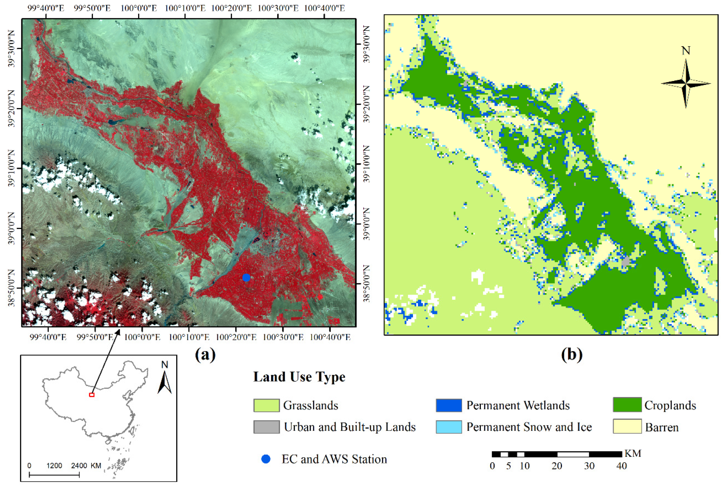
2.1. Study Area

The Heihe River Basin (HRB) is the second-largest inland river basin in the arid region of northwest China. The study area is located in an oasis–desert region in the middle reaches of the HRB and is distributed in a range of about 150 km × 150 km. The elevation ranges from 2000 to 3000 m above sea level (a.s.l.), and the annual precipitation is 100 to 250 mm. Maize is the main crop of the irrigated fields that grows from April to October and consumes plenty of the limited water resources, covering approximately 12% of the entire HRB [22]. There is no crop in the fields from November to March.

Figure 1a shows the standard false-color composite image from the GF1 WFV3 sensor in 2016 with a spatial resolution of 16 m. The red part is the central area of the oasis, and the blue point is the location of the meteorological station. The land-use type extracted from the MCD12Q1 International Geosphere-Biosphere Programme (IGBP) product is shown in Figure 1b; this region is mainly covered by croplands, grasslands, barren areas, etc. The grassland in Figure 1b is primarily alpine meadow. It is close to the upper reaches of HRB, where the maximum altitude is approximately 5000 m a.s.l. and the minimum air temperature approaches −40 °C. Over the past few decades, many scientific experiments have been carried out to better understand the ecological and hydrological process of the Heihe river basin [23].

2.2. EC and AWS Data

The observation system of meteorological elements gradient of superstation installed in the Daman irrigated area continuously collects data using eddy covariance and automatic weather systems through the HiWATER projects [24,25]. The ground-based measurements from 2013 to 2016 of this site were used to validate the estimations.

The raw EC observations were processed by EdiRe software, including spike detection, lag correction of H₂O/CO² relative to the vertical wind component, sonic virtual temperature correction, coordinating rotation, correction for density fluctuation, and frequency response correction. The half-hourly sensible heat flux (H) and latent heat flux (LE) were provided in the final released EC measurements.

The automatic weather system (AWS) observations were provided at every 10 min frequency, including the surface net radiation (Rn), the soil heat flux (G) measured using soil heat flow plate at a depth of 6 cm underground, mean soil temperature measured at the depths of 2 to 4 cm underground, soil moisture at different depths, wind velocity, air temperature and humidity at different heights, etc. The AWS measurements were averaged to 30 min frequency to keep consistent with the eddy data. The soil heat flow plate measured G was corrected by the Averaging Soil Thermocouple Probe (TCAV) [26] method based on the mean soil temperature and soil moisture measurements.

To solve the energy non-closure, the Bowen ratio correction method was adopted under the assumption that the ratio of latent heat to sensible heat is constant before and after closure correction [27]. Finally, the mean diurnal variation (MDV) method was used to fill the latent heat gaps to obtain continuous daily evapotranspiration measurements [28]. The average yearly ET from 2013 to 2016 is 759.5 mm, which is close to the value of 760.5 mm at the same site, according to Zhou et al. (2018) [29].

2.3. MODIS and CMADS Data

The MODIS remote sensing products, including the 500 m resolution daily land surface reflectance (MOD09GA) and 1 km resolution land surface temperature (MOD11A1), were used for ET model calculation. The Normalized Difference Vegetation Index (NDVI) was computed based on the near-infrared and red bands reflectance. This study also used the version 4 SSEBop Monthly Evapotranspiration product for comparison (From https://earlywarning.usgs.gov in 1 October 2020). As reported, it improves ET’s spatial accuracy by subdividing and modeling each MODIS tile into 25 units [15].

To eliminate the noise caused by cloud on the vegetation index, the Savitzky–Golay filtering was employed to process the daily NDVI. The upper envelope defined by the local maximum was detected to obtain a new NDVI time series. The leaf area index (LAI) and fractional vegetation cover (fv) were calculated using the empirical formulations calibrated based on NDVI and observed values in the same study area [1].

The version 1.1 CMADS datasets (From http://www.cmads.org in 1 October 2020) contain the daily averaged wind speed at 10 m height (m/s), the daily maximum and minimum air temperature (T_max and T_min, k), daily mean air temperature (T_mean, k), and daily mean relative humidity (RH) and solar radiation (R_s, MJ∙m⁻²∙d⁻¹) with 25 km resolution. The MOD11A1 and CMADS data were interpolated to a spatial resolution of 500 m by the bilinear method [21]. As the Penman–Monteith reference evapotranspiration equation needs the wind speed at the height of 2 m (u₂), the CMADS wind velocity was transformed into this height using the wind profile equation [30].

2.4. Methods

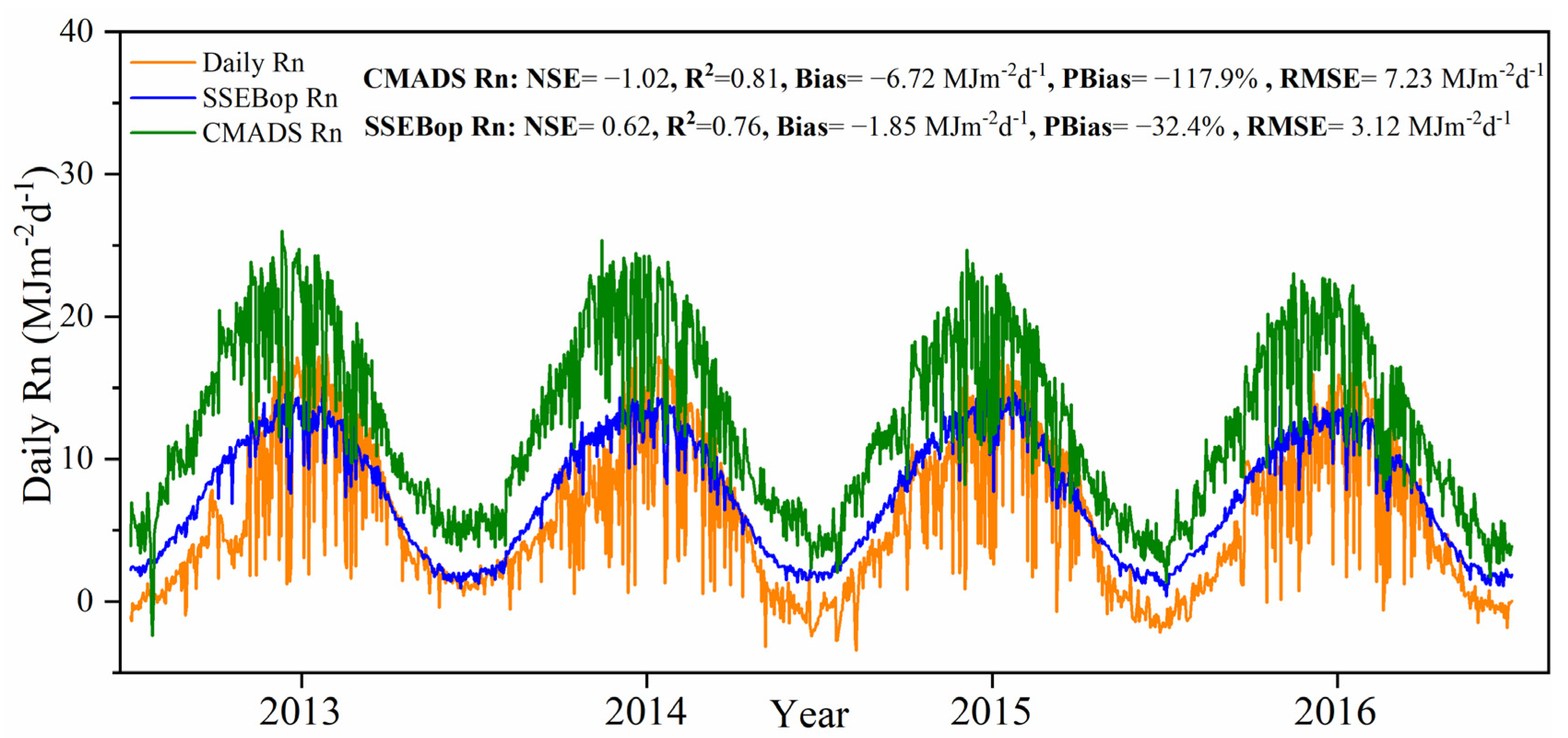
2.4.1. Daily Net Radiation

The daily net radiation can be expressed as the difference between the incoming net shortwave radiation (R_nsd) and the outgoing net longwave radiation (R_nl):

$$R_n=R_{nsd}-R_{nl}$$

(1)

$$R_{nsd}=(1-\alpha )R_s$$

(2)

where α is the albedo and was set as 0.23 for the hypothetic grass reference crop, and R_s is the solar radiation that can be derived from CMADS. The outgoing net longwave radiation (R_nl) was computed based on the daily maximum and minimum air temperature, daily mean vapor pressure, and the extraterrestrial solar radiation (R_a), according to Senay et al. (2018) [16].

Senay et al. [16] introduced a new modification to estimate the solar radiation by replacing the clear-sky with the ”average-sky” condition; k_Rs is the adjustment coefficient and ranges from 0.16~0.19.

$$R_s=R_a\times k_{Rs}\times \sqrt{T_{\max }-T_{\min }}$$

(3)

The average-sky condition assumes a given pixel in a given day will be subjected to an average cloud cover for the rest of the day despite the clear-sky condition during the instantaneous moment of satellite overpass, avoiding a general overestimation of the net radiation, which would lead to an overestimation of ET [16]. The two approaches for solar radiation computation were compared with the AWS measured ground truth to determine a better solution.

2.4.2. RSPMPT Model

The RSPMPT model computes the total latent heat flux as the sum of the transpiration from the vegetation canopy [31] and the soil surface evaporation [32]. The main formula will vary depending on whether the wet canopy evaporation term is distinguished [17,18]. In this study, the simple form was used and calculated as follows:

$$\lambda ET=\frac{\Delta R{n}_c+\rho C_p\frac{e_s-e_a}{r_a}}{\Delta +\gamma \left(1+\frac{r_c}{r_a}\right)}+\left[\left(1-f_{wet}\right)f_{sm}+f_{wet}\right]{\alpha }_{pt}\frac{\Delta }{\Delta +\gamma }\left(R{n}_s-G\right)$$

(4)

where R_nc, R_ns, and G are the daily net radiation (W·m⁻²) over canopy and soil surface and the soil heat flux (W·m⁻²), respectively. R_nc and R_ns were estimated by the fractional vegetation cover (fv) along with the net radiation, G was estimated by the ratio of soil heat flux to net radiation according to Su (2002) [5], λ is the latent heat of evaporation of water, Δ is the slope of the saturation vapor pressure versus temperature curve [30], γ is the psychrometric constant of ~0.066 (Kpa·K⁻¹), ρ is the air density (kg·m⁻³), C_p is the specific heat of the air (J·kg⁻¹·K⁻¹), and e_s and e_a are the saturated and actual vapor pressures (Kpa) and calculated by the daily mean air temperature and relative humidity (RH) from CMADS data. The relative surface wetness (f_wet) is used to determine whether the surface is wet or not and is equal to RH⁴. The f_sm is a soil moisture constraint used as an indicator of surface soil moisture. The coefficient α_pt is an empirical multiplier and was initially set to 1.26 for well-watered surfaces. The canopy resistance r_c (s/m) was found to vary with different environmental variables and was modeled as a product of the response functions to the environmental factors according to Jarvis’s model [33]. As soil moisture is not available in CMADS data, the solar radiation (f_sd), the vapor pressure deficit (f_vpd), and the air temperature (f_ta) factors were considered to scale the minimum canopy resistance (r_cmin) as follows:

$$r_c=\frac{r_{c\min }}{\mathrm{LAI}}\times f_{sd}\times f_{vpd}\times f_{ta}$$

(5)

The r_cmin was set as 36.6 s/m, which was optimized by MODIS and meteorological data in the same research area [34]. The aerodynamic resistance r_a (s/m) controls heat and water vapor transfer from the evaporating surface into the air above the canopy. It was calculated mainly based on the surface aerodynamic roughness and the daily wind velocity from CMADS. The RSPMPT model can thoroughly explain how plants’ transpiration rate varies with the increase or decrease in the environmental constraints under different conditions [35].

2.4.3. SSEBop Model

The SSEBop model assumes that the available net radiation mostly drives the surface energy balance process. Differences in land surface temperature can quantify a decline in ET due to water stress and other factors. SSEBop directly estimates pixel-based actual evapotranspiration (ET_a) by multiplying the ET fraction (ET_f) and reference ET (ET_r) as follows [15]:

$$E{T}_a=E{T}_f\times k_{\max }\times E{T}_r$$

(6)

where the k_max is the coefficient that scales the grass reference ET (ET_r) into the level of a maximum ET experienced by an aerodynamically rougher crop, and a recommended value for k_max is 1.2. The ET_r is calculated using the FAO-56 PM equation with the support of CMADS daily meteorological parameters [30].

$$E{T}_r=\frac{0.408\Delta (R_n-G)+\gamma \frac{900}{T_{mean}}{u}_2(e_s-e_a)}{\Delta +\gamma \left(1+0.34u_2\right)}$$

(7)

The ET fraction is a critical parameter for the actual ET computation in SSEBop, and is calculated as:

$$E{T}_f=1-\frac{T_s-T_c}{dT}$$

(8)

where the T_s is the MODIS land surface temperature; dT is a predefined temperature difference (K) between the “hot-dry” and “wet-cold” surfaces for each pixel and calculated as:

$$dT=\frac{R_n\times r_{ah}}{\rho \times C_p}$$

(9)

where r_ah is the aerodynamic resistance to heat flow from a hypothetical bare and dry surface (110 sm⁻¹), and the minimum value of dT is recommended as 6 K, reducing the ET uncertainty in cold climates. The T_c is the estimated T_s at the idealized “cold-wet” limit for each pixel and computed as:

$$T_c=c\times T_{\max }$$

(10)

$$c=\frac{T_{s\_cold}}{T_{\max }}$$

(11)

where c is a scene-specific factor that relates air temperature to T_{s_cold}, which is the average land surface temperature on a well-watered, fully transpiring vegetation surface, T_{s_cold} is obtained on all pixels where NDVI is greater than or equal to 0.7 in the image of a particular day [36]. If no pixels in the images of some days meet the NDVI conditions, the median value of all the effective c values within that year is used to replace the c value of those images. The minimum ET_f is set to 0. The maximum ET_f is 1.05, and the ET_f exceeding 1.3 is suspected of being contaminated by clouds and is filled through temporal interpolation by assuming linear relationships between two consecutive satellite dates. The SSEBop model eliminates the subjectivity and uncertainty that could be introduced during manual hot and cold reference selection, and more details can be found in [14,15,16,37,38].

3. Results

3.1. Daily Net Radiation

Daily (24 h) net radiation (Rn) is the energy boundary condition of the two models. The two approaches, one computed from the CMADS solar radiation (CMADS Rn), the other from the SSEBop equations under the “averaged sky” assumption (SSEBop Rn), were compared with the AWS measured daily net radiation. Generally, both the two methods could reflect the annual change of daily net radiation. However, there was an evident overestimation of daily net radiation based on the CMADS solar radiation, which had a higher root mean square error (RMSE) of 7.23 MJ∙m⁻²∙d⁻¹. In contrast, the daily net radiation from SSEBop had a lower RMSE of 3.12 MJ∙m⁻²∙d⁻¹ from 2013 to 2016. Figure 2 also shows the overall Nash–Sutcliffe efficiency (NSE), coefficient of determination (R²), mean bias error (bias), and percent bias (PBias) statistics for daily net radiation estimations. The NSE value close to 1 represents the overall high simulation accuracy of the model. The negative bias and PBias values indicated that both the two approaches overestimated daily net radiation. The bias error can be removed by applying the bias correction. It was found that both the NSE and RMSE improved after bias correction for the two approaches. The NSE increased to 0.77 and 0.72, and the RMSE decreased to 2.51 and 2.66 MJ∙m⁻²∙d⁻¹ for SSEBop and CMADS Rn, respectively. It can be concluded that although the SSEBop Rn slightly overestimated the daily net radiation, it had lower RMSE, better NSE than those of CMADS Rn before or after the bias correction. As the assessment of outgoing longwave radiation had the same formula, the overestimation of CMADS Rn primarily resulted from the uncertainties of the solar radiation provided by CMADS data. As reported by Santhi et al. (2001) [39], the model performance was considered to be acceptable if the NSE and R² were larger than 0.5 and 0.6, respectively. It is more convenient to compute daily net radiation from CMADS data when there is no site of observed sunshine duration. The SSEBop Rn approach was chosen to drive the two models for actual evapotranspiration simulation for its higher accuracy.

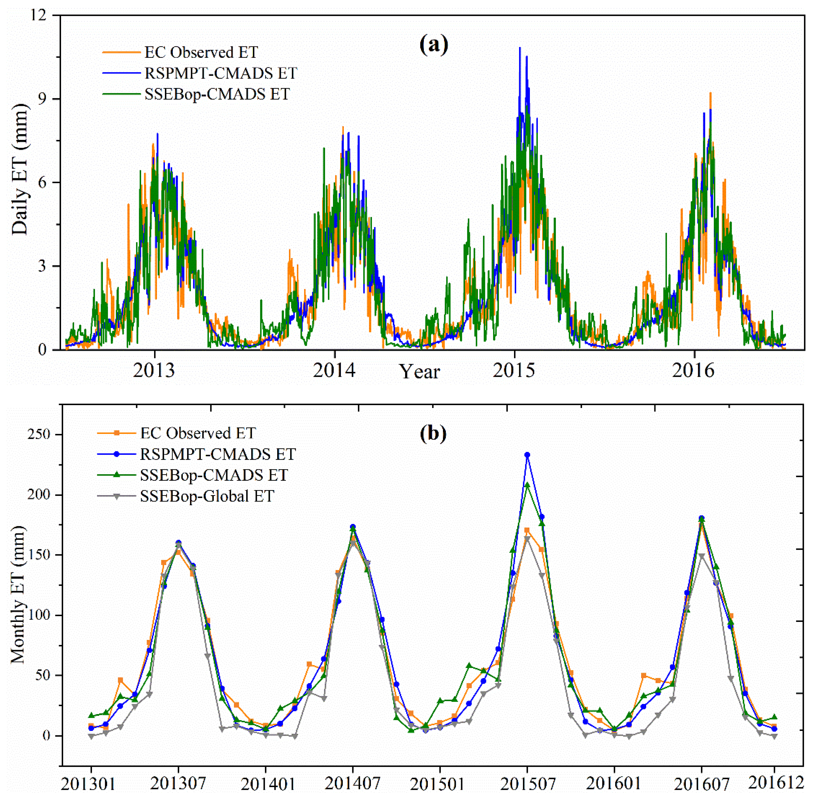
3.2. Validation of the Estimated ET with EC Measurements

The daily ET computed from RSPMPT, SSEBop with CMADS data, and derived from the version 4 SSEBop monthly global evapotranspiration product (hereafter, RSPMPT-CMADS, SSEBop-CMADS, SSEBop-Global) were compared with the eddy covariance system measured ET from 2013 to 2016 (Figure 3 and

Table 1. The overall performance statistics of daily and monthly ET estimations from 2013 to 2016.

Years	Temporal Scale	Methods	NSE	R2	Bias (mm)	RMSE (mm)	PBias (%)
2013–2016	Daily	RSPMPT-CMADS	0.84	0.86	0.03	0.78	1.41
		SSEBop-CMADS	0.78	0.81	0.01	0.90	0.59
	Monthly	RSPMPT-CMADS	0.93	0.95	0.86	14.3	1.35
		SSEBop-CMADS	0.93	0.94	0.34	13.7	0.53

).

As shown in Figure 3a and Table 1, both the RSPMPT-CMADS and SSEBop-CMADS showed a good performance of daily ET compared to the ground truth. Overall, the performance of RSPMPT with locally calibrated parameters (fv and LAI) was slightly better than that of SSEBop, with higher NSE (0.84 vs. 0.78) and R² (0.86 vs. 0.81), lower RMSE (0.78 mm·d⁻¹ vs. 0.90 mm·d⁻¹), although it had higher bias (0.03 mm·d⁻¹ vs. 0.01 mm·d⁻¹) and PBias (1.41% vs. 0.59%) from 2013 to 2016. Figure 3b shows the change process of monthly ET derived from different approaches and the EC observations. All the methods have the potential to deliver consistent changes in ET at different crop phenological stages. On the monthly scale, the NSE and R² of the two methods became higher, and the RMSE was close; the RSPMPT still had higher bias and PBias than SSEBop. Unlike other years, both the two models tended to overestimate ET from June to August in 2015.

Table 2. Averaged measured and estimated ET in different crop growth stages from 2013 to 2016.

Month	Measured Average	RSPMPT-CMADS ET (mm)		SSEBop-CMADS ET (mm)		SSEBop-Global ET (mm)
		Estimated Average	PBias (%)	Estimated Average	PBias (%)	Estimated Average	PBias (%)
Nov–Feb	12.2	7.9	34.9	15.6	−28.0	3.6	70.3
Mar	40.7	24.5	39.8	37.9	6.7	5.9	85.4
Apr–May	53.6	52.5	2.1	43.2	19.4	31.3	41.5
Jun–Aug	143.4	152.4	−6.3	151.0	−5.3	139.3	2.8
Sep–Oct	66.5	65.4	1.5	58.0	12.8	40.9	38.5

shows the statistics of averaged measured and estimated ET in different crop growth stages from 2013 to 2016. From November to February, there is no crop in the field during the cold and dry winter, and the croplands have little water or energy for evaporation. In this study area, spring agricultural irrigation was carried out in mid-March. Due to the increase of soil moisture content, farmland ET gradually began to increase. In March, the average ET approached 40.7 mm, and SSEBop-CMADS had the best estimates, with a PBias of 6.7%. In contrast, the SSEBop-Global showed an apparent underestimation (with an average ET of 5.9 mm and a PBias of 85.4%). As crop growth requires a lot of irrigation during the growing season, both vegetation transpiration and crop evaporation begin to rise. Much higher ET values were found in both estimations or observations during the crop peak growing season from June to August. The three approaches had similar estimation accuracy, with PBias from −6.3% to 2.8% during this period. At the early and late stages of crop growth, roughly during April to May and September to October, the cropland ET was lower than that in peak growing season, and RSPMPT-CMADS had the best performance.

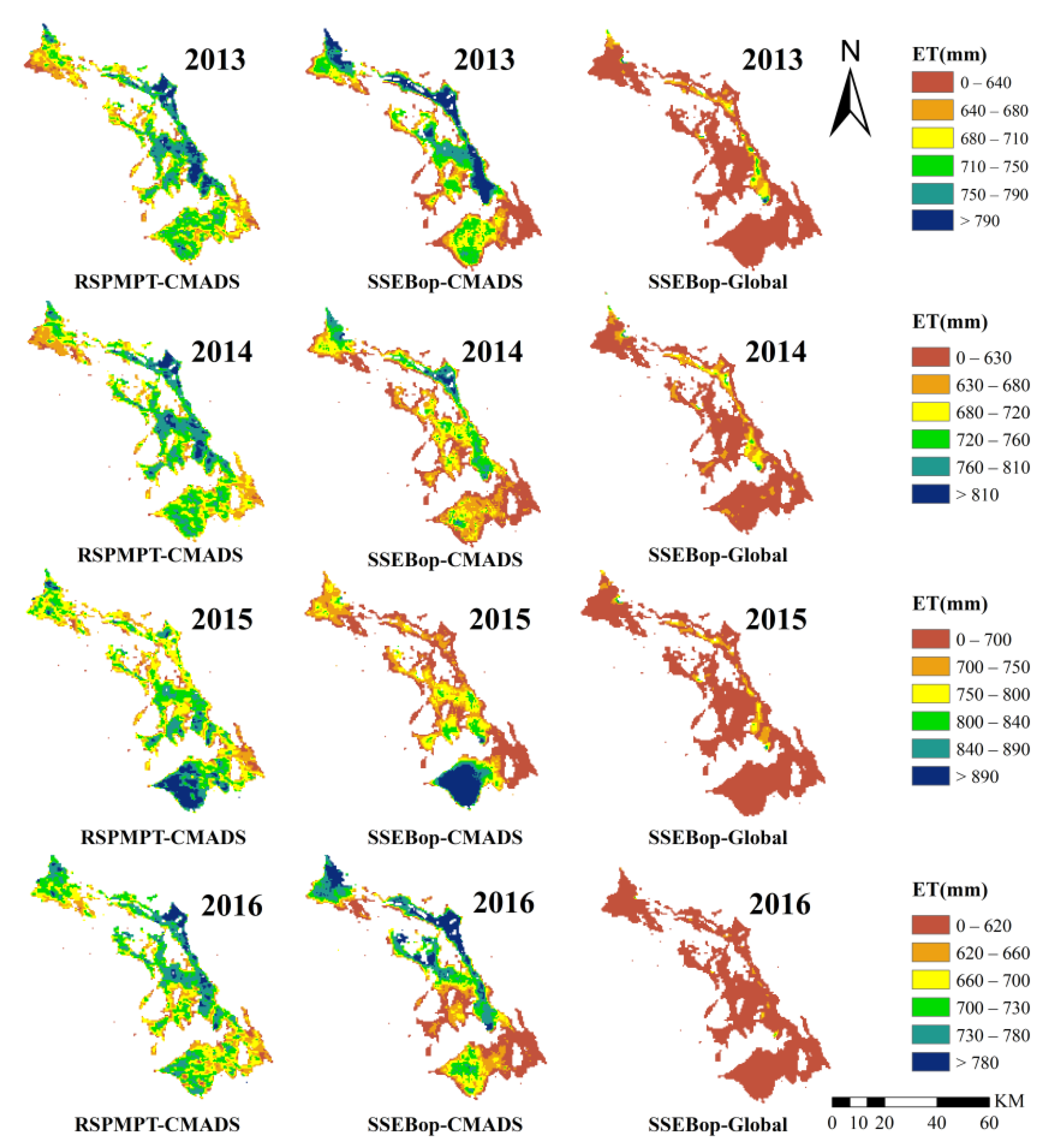
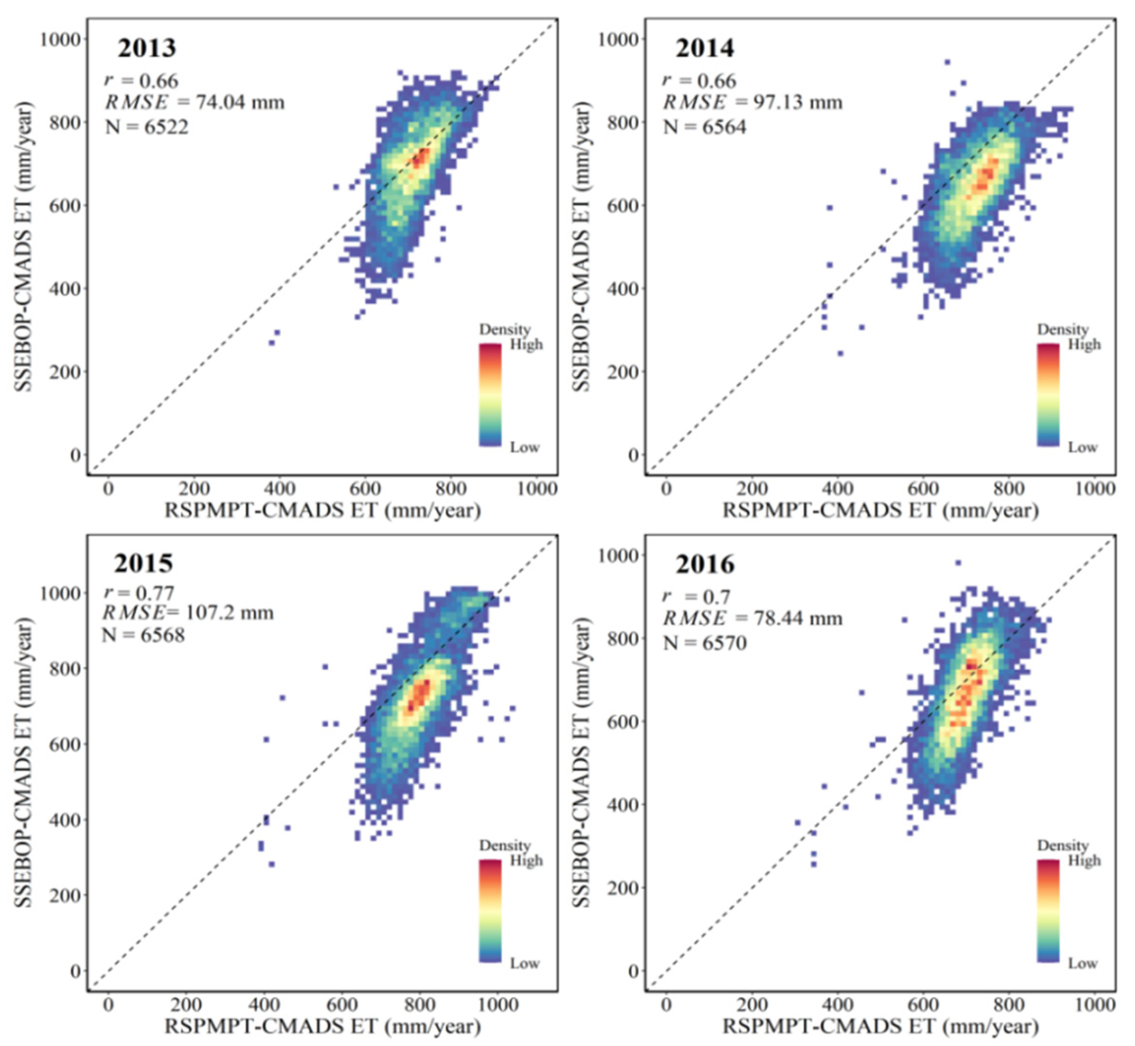
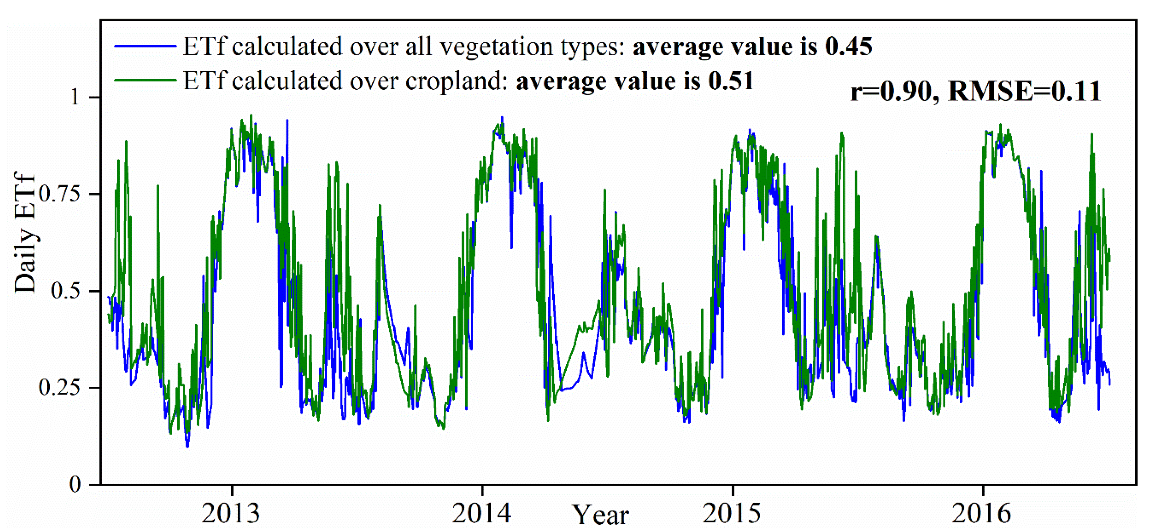
3.3. Spatial Comparisons of the Estimated ET

Figure 4 shows the cropland’s evapotranspiration maps from 2013 to 2016 in the study area. The evapotranspiration spatial distribution obtained by different methods was inconsistent. The RSPMPT-CMADS and SSEBop-CMADS had more similar ET patterns, while the SSEBop-Global showed lower annual ET throughout this region.

Although the underlying surface is homogeneous, the maps demonstrate the spatial heterogeneity of evapotranspiration, which may be caused by the differences in irrigation intensity, irrigation types, crop types and conditions, and other environmental factors. In general, the RSPMPT-CMADS had spatially higher ET than the other two approaches and mostly ranged from 680~810 mm/y in the years 2013, 2014, and 2016. In 2015, both the RSPMPT-CMADS and SSEBop-CMADS had spatially more extensive ET than those of other years in the Daman irrigated area around the EC and AWS station.

The density scatter plots of the RSPMPT-CMADS and SSEBop-CMADS estimated annual croplands evapotranspiration from 2013 to 2016 are displayed in Figure 5. There was a moderate correlation between the two models’ estimations with the correlation coefficients between 0.66 to 0.77 based on the statistic from more than 6500 pixels. The RSPMPT-CMADS computed higher ET than that of the SSEBop-CMADS from 2013 to 2016 in the study area. Relative large RMSE values were found between the two models, ranging from 74.0 to 107.2 mm/year, indicating the two approaches’ different performances at spatial scale. The ET density told that more pixels were concentrated in evapotranspiration between 600~800 mm/year for the two methods, and the highest density of annual ET was around 700 mm/y for the croplands.

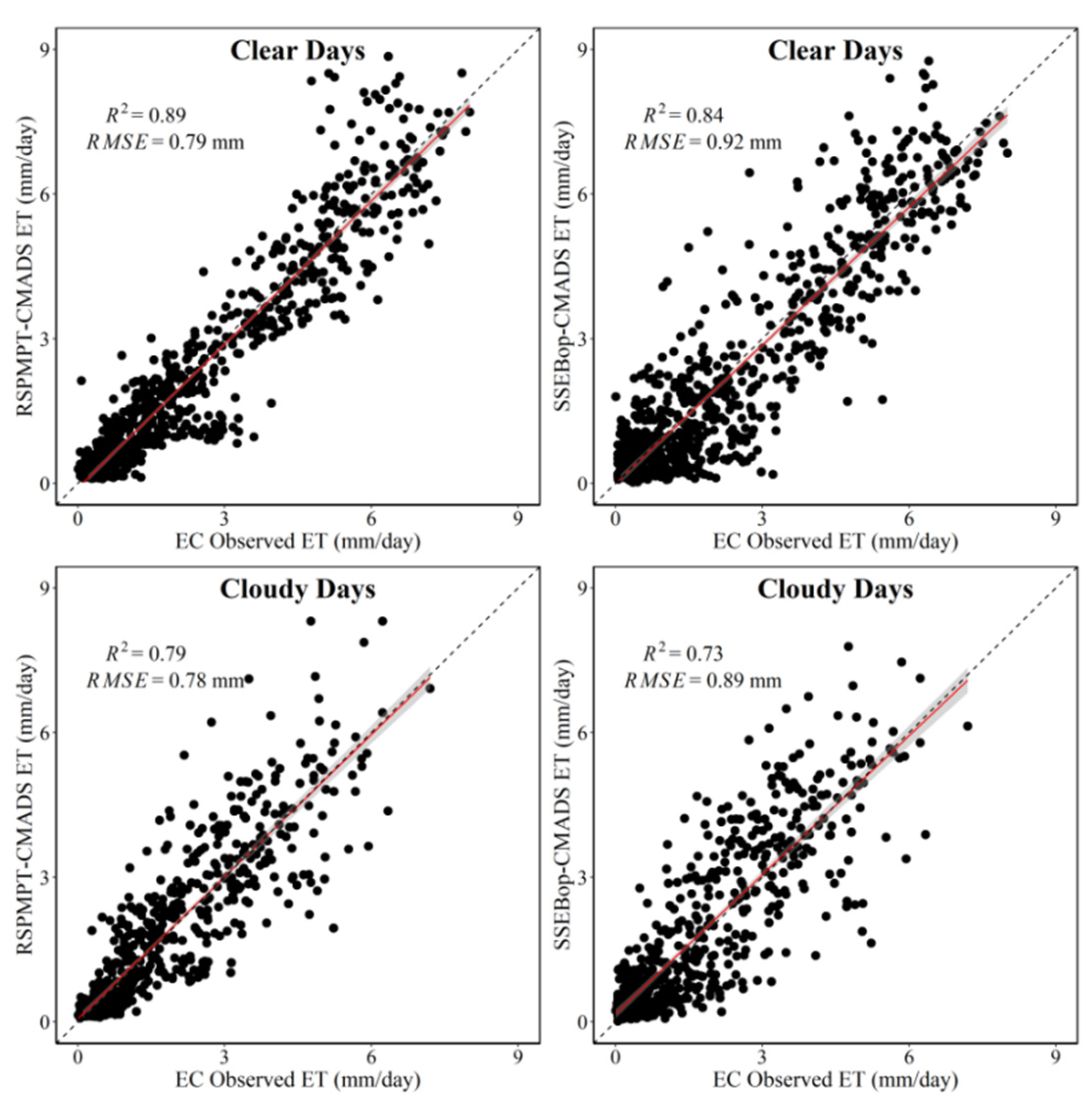
3.4. The Models’ Performances for Cloudy Days

The most critical part to continuously monitor ET by remote sensing is to reconstruct the ET time series of cloudy days. The LST quality control documents in the MOD11A1 product were used to determine whether there are clear pixels or not around the EC site. Figure 6 and

Table 3. The other statistics for the models estimated ET on clear and cloudy days.

Days	Number	RSPMPT-CMADS			SSEBop-CMADS
		NSE	Bias (mmd−1)	PBias (%)	NSE	Bias (mmd−1)	PBias (%)
Clear Days	805	0.86	0.08	3.3	0.82	0.11	4.4
Cloudy Days	656	0.73	−0.04	−2.2	0.65	−0.11	−6.5

show the scatter plots and the statistics for the estimated ET by the two models on clear and cloudy days. From 2013 to 2016, there were 805 clear days and 656 cloudy days. The RSPMPT-CMADS and SSEBop-CMADS models had the coefficients of determination (R²) of 0.89 and 0.84 on clear days. On cloudy days, both models’ performance decreased slightly with R² of 0.79 and 0.73, respectively. However, the root mean square errors (RMSE) of the two models were low on both clear and cloudy days. The relatively high NSE and R² for both clear and cloudy days indicates the effectiveness of the two models for estimating evapotranspiration continuously over irrigated fields. From the bias and PBias, both the two models showed slight overestimation of ET on cloudy days.

Table 4. The canopy resistance (r_c) and ETf during the crop growing and non-growing seasons.

Month	Days	Number	rc (s/m)	ETf
Apr to Oct	Clear Days	504	160.1	0.61
	Cloudy Days	352	271.9	0.63
Nov to Mar	Clear Days	301	3328.2	0.42
	Cloudy Days	304	4205.7	0.47

shows the canopy resistance (r_c) and ET_f during the crop growing and non-growing seasons, which are the critical parameters of RSPMPT and SSEBop, respectively. Lower canopy resistance and higher ET_f were found in the growing season. In both growing and non-growing seasons, the daily canopy resistance on cloudy days was higher than on clear days. The solar radiation environmental stress increased due to the decrease of the downward solar shortwave radiation on cloudy days. However, the ET_f in SSEBop models did not show a significant decline on cloudy days. Therefore, in contrast, SSEBop is more likely to overestimate ET on cloudy days, with a PBias of −6.5%, which is lower than that of the RSPMPT (−2.2%). The RSPMPT estimated ET on cloudy days using smoothed NDVI and the meteorological data, whereas the SSEBop model estimated ET by filling the ET_f on cloudy days through temporal interpolation based on adjacent valid ET_f values. The ET_f variations caused by the changes of environmental factors are not considered in the interpolation process.

3.5. The Models’ Performances for Growing Season

It is essential to identify the evapotranspiration estimation accuracy in crop growing season when the model is used in crop water-consuming monitoring [40].

Table 5. The error statistics for the ET estimated by RSPMPT-CMADS and SSEBop-CMADS models.

Year	Statistics	Growing Season		Non-Growing Season
		RSPMPT-CMADS	SSEBop-CMADS	RSPMPT-CMADS	SSEBop-CMADS
2013–2016	NSE	0.74	0.67	0.35	0.10
	R2	0.78	0.92	0.59	0.30
	RMSE (mmd−1)	0.94	1.07	0.47	0.59
	Bias (mmd−1)	−0.11	0.07	0.23	−0.06
	PBias (%)	−3.42	2.23	37.48	−11.62

shows the error statistics for the evapotranspiration from RSPMPT-CMADS and SSEBop-CMADS models during growing and non-growing seasons. The simulation accuracy of the two models in the crop growing season is significantly better than that in the non-growing season. The RSPMPT-CMADS had higher NSE and R², and lower RMSE than the SSEBop-CMADS in both growing and non-growing seasons. However, the SSEBop-CMADS had better bias and PBias, especially in the non-growing season, and the RSPMPT-CMADS significantly underestimated cropland evapotranspiration. During the non-growing season, soil water evaporation is the primary source of evapotranspiration. The canopy resistance in the RSRMPT model is substantial (~5000 s/m) as the LAI is very low, so the ET from vegetation decreases. The soil transpiration is scaled from its potential level based on the soil moisture constraint and relative surface wetness. The soil moisture constraint estimated by vapor pressure has more uncertainties than that estimated by soil moisture [41]. It takes a long time and a more extensive range for surface soil moisture change to affect the water vapor pressure near the surface. The soil moisture constraint estimated by vapor pressure is more suitable for evapotranspiration estimation over large scales and long time intervals (e.g., eight days). In contrast, the pixel-based land surface temperature can be sensitive to soil moisture. The irrigated fields with higher soil moisture always experience cooler land surface temperature than the dryland fields [40]. The better bias proved that when soil moisture changes in the non-growing season (e.g., irrigation before sowing or after rainfall), the SSEBop model has more potential to reflect the evolution of evapotranspiration. It is consistent with the statistics shown in Table 2 that the SSEBop model can effectively reflect the increase of evapotranspiration caused by irrigation around the AWS station before sowing in March.

4. Discussion

Both RSPMPT and SSEBop models are easy to apply at a regional scale because they do not need to compute each intermediate variable in the SEB equation and can compute daily ET without instantaneous estimations. Since CMADS directly provides daily meteorological parameters necessary for the two models, it is of great convenience to simulate ET by combining the two models with the CMADS data. The validation of daily net radiation shows that the overestimation of CMADS solar radiation leads to a lower negative percent bias (PBias), indicating the apparent overestimation of net radiation. It is recommended to use the maximum and minimum air temperature to compute the daily net radiation by CMADS under “average-sky” conditions.

As can be seen in Figure 3, both the two models overestimated ET in 2015 significantly. Since the daily net radiation estimations do not show apparent annual variation, the CMADS daily meteorological variables were further explored and compared to the AWS averaged measurements from 2013 to 2016. As shown in Figure 7, from 2013 to 2016, the wind speed was apparently higher than the other years. In addition, the air temperature (minimum, maximum, and averaged) and air pressure were slightly higher in 2015 than those in other years. Significantly higher wind speed may compute lower aerodynamic resistance and lead to higher canopy transpiration for RSPMPT and higher reference evapotranspiration for SSEBop.

In previous studies, the two models’ uncertainties have been thoroughly discussed [18,42]. The sensitivity analysis of the RMPMPT model showed that the canopy resistance was responsible for 95.7% of the variability in the ET results [18]. In this study, the Savitzky–Golay filtering was used to process the daily NDVI smoothing. Daily NDVI calculated the daily LAI, and the LAI and meteorological data estimated the canopy resistance. RSPMPT is easier to use because it does not require land surface temperature input. However, the parameters, LAI, and the fractional vegetation cover (fv) were also critical and sensitive for the model calculation [1,43]. At present, statistical regression methods are used to optimize the estimation of these parameters. In this study, the regression formula with local calibration in the same study area was used. ET estimation accuracy was improved compared with other LAI and fv empirical formulas (not shown).

The SSEBop model is sensitive to input variables, land surface temperature (LST) and reference ET, and parameters, differential temperature (dT), and maximum ET scalar (k_max), particularly during the non-growing season and in dry areas [42]. The necessary process of the SSEBop model is to determine the cold pixel coefficient (C factor) within the image range and calculate the “hot/dry” and “cold/wet” surface temperatures at the two idealized reference conditions for each pixel in the same period. Ji et al. (2019) defined the cold pixel as NDVI > 0.7 for vegetation cover based on the knowledge and experience with the use of satellite-derived vegetation indices in ET modeling and mapping [36]. In this study, the cold pixels were determined over the cropland, mostly located in the middle reach of the Heihe river basin. Besides, cold pixels can also be determined over all vegetation types within the image. For comparison, Figure 8 shows that the C values calculated over croplands were slightly higher than those of C calculated over all vegetation types. By comparing the minimum, maximum, middle, and average values of the C factors calculated by the two methods, it was found that the maximum value was almost the same. In contrast, the C factor’s minimum values had a large gap, and the median and average values had a slight gap, which showed that the C factor calculated by all vegetation types was lower.

According to Senay et al. (2018) [16], the median value of the C factor within one year is suggested to replace the image without “cold/wet” pixels. In farmland area, the period when “cold/wet” pixels cannot be found is mostly non-growing season. A lower median value of the C factor may lead to a lower ET fraction (ET_f) value in this period. Figure 9 shows the daily ET_f values from 2013 to 2016, and the lowest values calculated over all vegetation types concentrated on non-growing season. A lower ET_f means a lower ET estimate. From 2013 to 2016, the pixel-averaged cropland ET estimated by C factor calculated over all vegetation types was about 40 mm lower than that estimated by C factor calculated over croplands only. The possible reason is that alpine meadow surface temperature in high-altitude areas is lower than that of farmland. Simultaneously, the spatial resolution of CMADS is coarse, and the difference of maximum temperature between the two types is not as evident as that of surface temperature. It is worth noting that the version 4 SSEBop ET product is also significantly underestimated in the non-growing season, which eventually leads to the underestimation of annual crop ET. This product improves the spatial accuracy of ET by subdividing and modeling each MODIS tile into 25 units. However, it is also an extensive area, close to 450 km, due to the MODIS scan width of 2330 km. To a large extent, if the altitude, climate, and vegetation types vary significantly in different parts, the selection of vegetation types is also crucial for determining cold pixels.

5. Conclusions

Monitoring cropland ET continuously is essential for agricultural water resources management and drought monitoring, especially for the arid areas with limited water resources. Remote sensing-based ET models can simulate the spatiotemporal features of ET.

This study’s main objective was to evaluate the performance of the RSPMPT and SSEBop models driven by MODIS and CMADS data over irrigated fields in the Heihe river basin of China. The eddy covariance observed ET was used to make a quantitative evaluation of the models.

This study demonstrated that both the RSPMPT and SSEBop models produced robust daily ET results. Overall, the SSEBop model’s performance was slightly inferior to that of the RSPMPT model with local calibration. The performance result also strengthens the useful application of the CMADS data for daily ET estimation. The solar radiation is overestimated, and the wind speed has an apparent interannual mutation from 2013 to 2016 in the study area. This study also found that the cold pixel coefficients (C factor) in SSEBop determined over all vegetation types or croplands caused different ET estimation. The ET estimated using C factors from all vegetation types was lower than using C factors from croplands. During the non-growing seasons, the C factor cannot be determined from croplands. The C factor calculated over alpine meadow was too low for the croplands during this period due to the increase of soil evaporation caused by the irrigation before sowing. It is more reasonable to replace the C factor in non-growing seasons with the medium C factor values over croplands of one year. It proved that the selection of vegetation types is also crucial for determining cold pixels in the SSEBop model if the altitude, climate, and vegetation types vary significantly in different parts of the research area. On cloudy days, the SSEBop model is more likely to overestimate evapotranspiration than the RSPMPT model because its ET_f time expansion method does not consider environmental factors’ impact. During the non-growing season, the SSEBop model was more sensitive to the change of evapotranspiration caused by irrigation before sowing, which had a lower bias, and the random error accounted for the most proportion of total errors.

To conclude, this is the first comprehensive validation and comparison of the two simple and popular ET models driven by MODIS and CMADS data (e.g., RSPMPT-CMADS and SSEBop-CMADS) over irrigated fields in the Heihe river basin. The two approaches both had the potential to model continuous ET over irrigated fields at spatiotemporal scales and reflect the heterogeneity of croplands ET caused by different crop species, crop growth, and irrigation amount. The SSEBop is more practical over a large area because it has more capacity to capture the ET heterogeneity of irrigated fields and needs less empirical coefficient, especially in the absence of measured data, to optimize the RSPMPT model parameters.

References

1. Li, Y.; Huang, C.; Hou, J.; Gu, J.; Zhu, G.; Li, X. Mapping daily evapotranspiration based on spatiotemporal fusion of ASTER and MODIS images over irrigated agricultural areas in the Heihe River Basin, Northwest China. Agric. For. Meteorol. 2017, 244–245, 82–97. [Google Scholar] [CrossRef]
2. Yan, H.; Wang, S.Q.; Billesbach, D.; Oechel, W.; Zhang, J.H.; Meyers, T.; Martin, T.A.; Matamala, R.; Baldocchi, D.; Bohrer, G.; et al. Global estimation of evapotranspiration using a leaf area index-based surface energy and water balance model. Remote Sens. Environ. 2012, 124, 581–595. [Google Scholar] [CrossRef] [Green Version]
3. Zhuang, Q.; Wu, B.; Yan, N.; Zhu, W.; Xing, Q. A method for sensible heat flux model parameterization based on radiometric surface temperature and environmental factors without involving the parameter KB−1. Int. J. Appl. Earth. Obs. 2016, 47, 50–59. [Google Scholar] [CrossRef]
4. Bastiaanssen, W.G.M.; Menenti, M.; Feddes, R.A.; Holtslag, A.A.M. A remote sensing surface energy balance algorithm for land (SEBAL). 1. Formulation. J. Hydrol. 1998, 212–213, 198–212. [Google Scholar] [CrossRef]
5. Su, Z. The Surface Energy Balance System (SEBS) for estimation of turbulent heat fluxes. Hydrol. Earth Syst. Sci. 2002, 6, 85–100. [Google Scholar] [CrossRef]
6. Allen, R.G.; Tasumi, M.; Morse, A.; Trezza, R.; Wright, J.L.; Bastiaanssen, W.; Kramber, W.; Lorite, I.; Robison, C.W. Satellite-Based Energy Balance for Mapping Evapotranspiration with Internalized Calibration (METRIC)—Applications. J. Irrig. Drain. Eng. 2007, 133, 395–406. [Google Scholar] [CrossRef]
7. Norman, J.M.; Kustas, W.P.; Humes, K.S. Source approach for estimating soil and vegetation energy fluxes in observations of directional radiometric surface temperature. Agric. For. Meteorol. 1995, 77, 263–293. [Google Scholar] [CrossRef]
8. Anderson, M. A Two-Source Time-Integrated Model for Estimating Surface Fluxes Using Thermal Infrared Remote Sensing. Remote Sens. Environ. 1997, 60, 195–216. [Google Scholar] [CrossRef]
9. Norman, J.M.; Anderson, M.C.; Kustas, W.P.; French, A.N.; Mecikalski, J.; Torn, R.; Diak, G.R.; Schmugge, T.J.; Tanner, B.C.W. Remote sensing of surface energy fluxes at 101-m pixel resolutions. Water Resour. Res. 2003, 39. [Google Scholar] [CrossRef] [Green Version]
10. Mu, Q.; Heinsch, F.A.; Zhao, M.; Running, S.W. Development of a global evapotranspiration algorithm based on MODIS and global meteorology data. Remote Sens. Environ. 2007, 111, 519–536. [Google Scholar] [CrossRef]
11. Yin, L.; Wang, X.; Feng, X.; Fu, B.; Chen, Y. A Comparison of SSEBop-Model-Based Evapotranspiration with Eight Evapotranspiration Products in the Yellow River Basin, China. Remote Sens. 2020, 12, 2528. [Google Scholar] [CrossRef]
12. Long, D.; Yan, L.; Bai, L.; Zhang, C.; Li, X.; Lei, H.; Yang, H.; Tian, F.; Zeng, C.; Meng, X.; et al. Generation of MODIS-like land surface temperatures under all-weather conditions based on a data fusion approach. Remote Sens. Environ. 2020, 246, 111863. [Google Scholar] [CrossRef]
13. Xu, T.; Liu, S.; Xu, L.; Chen, Y.; Jia, Z.; Xu, Z.; Nielson, J. Temporal Upscaling and Reconstruction of Thermal Remotely Sensed Instantaneous Evapotranspiration. Remote Sens. 2015, 7, 3400–3425. [Google Scholar] [CrossRef] [Green Version]
14. Senay, G.B.; Friedrichs, M.; Singh, R.K.; Velpuri, N.M. Evaluating Landsat 8 evapotranspiration for water use mapping in the Colorado River Basin. Remote Sens. Environ. 2016, 185, 171–185. [Google Scholar] [CrossRef] [Green Version]
15. Senay, G.B.; Bohms, S.; Singh, R.K.; Gowda, P.H.; Velpuri, N.M.; Alemu, H.; Verdin, J.P. Operational Evapotranspiration Mapping Using Remote Sensing and Weather Datasets: A New Parameterization for the SSEB Approach. J. Am. Water Resour. As. 2013, 49, 577–591. [Google Scholar] [CrossRef] [Green Version]
16. Senay, G.B. Satellite Psychrometric Formulation of the Operational Simplified Surface Energy Balance (SSEBop) Model for Quantifying and Mapping Evapotranspiration. Appl. Eng. Agric. 2018, 34, 555–566. [Google Scholar] [CrossRef] [Green Version]
17. El Masri, B.; Rahman, A.F.; Dragoni, D. Evaluating a new algorithm for satellite-based evapotranspiration for North American ecosystems: Model development and validation. Agric. For. Meteorol. 2019, 268, 234–248. [Google Scholar] [CrossRef]
18. Song, Y.; Jin, L.; Zhu, G.; Ma, M. Parameter estimation for a simple two-source evapotranspiration model using Bayesian inference and its application to remotely sensed estimations of latent heat flux at the regional scale. Agric. For. Meteorol. 2016, 230–231, 20–32. [Google Scholar] [CrossRef]
19. Meng, X.; Wang, H. Significance of the China Meteorological Assimilation Driving Datasets for the SWAT Model (CMADS) of East Asia. Water 2017, 9, 765. [Google Scholar] [CrossRef]
20. Hao, Y.; Baik, J.; Choi, M. Combining generalized complementary relationship models with the Bayesian Model Averaging method to estimate actual evapotranspiration over China. Agric. For. Meteorol. 2019, 279, 107759. [Google Scholar] [CrossRef]
21. Tian, Y.; Zhang, K.; Xu, Y.; Gao, X.; Wang, J. Evaluation of Potential Evapotranspiration Based on CMADS Reanalysis Dataset over China. Water 2018, 10, 1126. [Google Scholar] [CrossRef] [Green Version]
22. Wu, B.; Zhu, W.; Yan, N.; Xing, Q.; Xu, J.; Ma, Z.; Wang, L. Regional Actual Evapotranspiration Estimation with Land and Meteorological Variables Derived from Multi-Source Satellite Data. Remote Sens. 2020, 12, 332. [Google Scholar] [CrossRef] [Green Version]
23. Li, X.; Cheng, G.; Liu, S.; Xiao, Q.; Ma, M.; Jin, R.; Che, T.; Liu, Q.; Wang, W.; Qi, Y.; et al. Heihe Watershed Allied Telemetry Experimental Research (HiWATER): Scientific Objectives and Experimental Design. Bull. Am. Meteorol. Soc. 2013, 94, 1145–1160. [Google Scholar] [CrossRef]
24. Liu, S.; Li, X.; Xu, Z.; Che, T.; Xiao, Q.; Ma, M.; Liu, Q.; Jin, R.; Guo, J.; Wang, L.; et al. The Heihe Integrated Observatory Network: A Basin-Scale Land Surface Processes Observatory in China. Vadose Zone J. 2018, 17, 1–21. [Google Scholar] [CrossRef]
25. Liu, S.; Xu, Z.; Wang, W.; Jia, Z.; Zhu, M.; Bai, J.; Wang, J. A comparison of eddy-covariance and large aperture scintillometer measurements with respect to the energy balance closure problem. Hydrol. Earth Syst. Sc. 2011, 15, 1291–1306. [Google Scholar] [CrossRef] [Green Version]
26. Sanwangsri, M.; Hanpattanakit, P.; Chidthaisong, A. Variations of Energy Fluxes and Ecosystem Evapotranspiration in a Young Secondary Dry Dipterocarp Forest in Western Thailand. Atmosphere 2017, 8, 152. [Google Scholar] [CrossRef] [Green Version]
27. Twine, T.E.; Kustas, W.P.; Norman, J.M.; Cook, D.R.; Houser, P.R.; Meyers, T.P.; Prueger, J.H.; Starks, P.J.; Wesely, M.L. Correcting eddy-covariance flux underestimates over a grassland. Agric. For. Meteorol. 2000, 103, 279–300. [Google Scholar] [CrossRef] [Green Version]
28. Falge, E.; Baldocchi, D.; Olson, R.; Anthoni, P.; Tu, K. Gap filling strategies for defensible annual sums of net ecosystem exchange. Agric. For. Meteorol. 2001, 107, 43–69. [Google Scholar] [CrossRef] [Green Version]
29. Zhou, S.; Yu, B.; Zhang, Y.; Huang, Y.; Wang, G. Water use efficiency and evapotranspiration partitioning for three typical ecosystems in the Heihe River Basin, northwestern China. Agric. For. Meteorol. 2018, 253–254, 261–273. [Google Scholar] [CrossRef]
30. Allen, R.G.; Pereira, L.S.; Raes, D.; Smith, M. Crop evapotranspiration. In Guidelines for Computing Crop Water Requirements; Irrigation and Drainage Paper 56; FAO: Rome, Italy, 1998; p. 300. [Google Scholar]
31. Leuning, R.; Zhang, Y.Q.; Rajaud, A.; Cleugh, H.; Tu, K. A simple surface conductance model to estimate regional evaporation using MODIS leaf area index and the Penman-Monteith equation. Water Resour. Res. 2008, 44. [Google Scholar] [CrossRef]
32. Fisher, J.B.; Tu, K.P.; Baldocchi, D.D. Global estimates of the land-atmosphere water flux based on monthly AVHRR and ISLSCP-II data, validated at 16 FLUXNET sites. Remote Sens. Environ. 2008, 112, 901–919. [Google Scholar] [CrossRef]
33. Jarvis, P.G. The Interpretation of the Variations in Leaf Water Potential and Stomatal Conductance Found in Canopies in the Field. Philos. T. R. Soc. B. 1976, 273, 593–610. [Google Scholar]
34. Song, Y.; Wang, J.; Yang, K.; Ma, M.; Li, X.; Zhang, Z.; Wang, X. A revised surface resistance parameterisation for estimating latent heat flux from remotely sensed data. Int. J. Appl. Earth Obs. 2012, 17, 76–84. [Google Scholar] [CrossRef]
35. Zhuang, Q.; Wang, H.; Xu, Y. Comparison of Remote Sensing based Multi-Source ET Models over Cropland in a Semi-Humid Region of China. Atmosphere 2020, 11, 325. [Google Scholar] [CrossRef] [Green Version]
36. Ji, L.; Senay, G.B.; Velpuri, N.M.; Kagone, S. Evaluating the Temperature Difference Parameter in the SSEBop Model with Satellite-Observed Land Surface Temperature Data. Remote Sens. 2019, 11, 1947. [Google Scholar] [CrossRef] [Green Version]
37. Senay, G.B.; Schauer, M.; Friedrichs, M.; Velpuri, N.M.; Singh, R.K. Satellite-based water use dynamics using historical Landsat data (1984–2014) in the southwestern United States. Remote Sens. Environ. 2017, 202, 98–112. [Google Scholar] [CrossRef]
38. Senay, G.B.; Budde, M.E.; Verdin, J.P. Enhancing the Simplified Surface Energy Balance (SSEB) approach for estimating landscape ET: Validation with the METRIC model. Agric. Water Manag. 2011, 98, 606–618. [Google Scholar] [CrossRef]
39. Santhi, C.; Arnold, J.G.; Williams, J.R. Validation of the Swat Model on A Large River Basin with Point and Nonpoint Sources. J. Am. Water Resour. Assoc. 2001, 37, 1169–1188. [Google Scholar] [CrossRef]
40. Senay, G.B.; Gowda, P.H.; Bohms, S.; Howell, T.A.; Friedrichs, M.; Marek, T.H.; Verdin, J.P. Evaluating the SSEBop approach for evapotranspiration mapping with landsat data using lysimetric observations in the semi-arid Texas High Plains. Hydrol. Earth Syst. Sci. Discuss. 2014, 11, 723–756. [Google Scholar]
41. Purdy, A.J.; Fisher, J.B.; Goulden, M.L.; Colliander, A.; Halverson, G.; Tu, K.; Famiglietti, J.S. SMAP soil moisture improves global evapotranspiration. Remote Sens. Environ. 2018, 219, 1–14. [Google Scholar] [CrossRef]
42. Chen, M.; Senay, G.B.; Singh, R.K.; Verdin, J.P. Uncertainty analysis of the Operational Simplified Surface Energy Balance (SSEBop) model at multiple flux tower sites. J. Hydrol. 2016, 536, 384–399. [Google Scholar] [CrossRef] [Green Version]
43. Yang, Y.; Long, D.; Guan, H.; Liang, W.; Simmons, C.; Batelaan, O. Comparison of three dual-source remote sensing evapotranspiration models during the MUSOEXE-12 campaign: Revisit of model physics. Water Resour. Res. 2015, 51, 3145–3165. [Google Scholar] [CrossRef]
Figure 1. (a) The standard false-color composite image for the oasis–desert area from the GF1 WFV3 sensor in 2016; (b) the land-use type from MCD12Q1 IGBP class product.
Agriculture 11 00424 g001
Figure 2. Comparisons of daily net radiation estimated from different methods with AWS measured ground truth.
Agriculture 11 00424 g002
Figure 3. Comparisons of daily ET (a) and monthly ET (b) derived from different approaches with EC measured ground truth.
Agriculture 11 00424 g003
Figure 4. Annual accumulated evapotranspiration of the study area derived from the three approaches (RSPMPT-CMADS, SSEBop-CMADS, SSEBop-Global) from 2013 to 2016.
Agriculture 11 00424 g004
Figure 5. Density scatter plots of the RSPMPT-CMADS and SSEBop-CMADS estimated annual evapotranspiration from 2013 to 2016.
Agriculture 11 00424 g005
Figure 6. The scatter plots for the two methods (RSPMPT-CMADS and SSEBop-CMADS) estimated ET versus EC observed ET on clear and cloudy days.
Agriculture 11 00424 g006
Figure 7. The mean meteorological variables from monthly averaged CMADS daily data from 2013 to 2016 around the AWS station.
Agriculture 11 00424 g007
Figure 8. The minimum, maximum, median, and average values of C factors calculated over croplands and all vegetation types, respectively, in the SSEBop model.
Agriculture 11 00424 g008
Figure 9. The regional mean daily values of ET fraction (ETf) calculated over croplands and all vegetation types, respectively.
Agriculture 11 00424 g009