Construction and Experimental Verification of Sloped Terrain Soil Pressure-Sinkage Model

Abstract

The construction of a scientific and effective soil pressure-sinkage model under sloped terrain condition has important guiding significance for the investigation of the soil compaction effect. It is also important for the theoretical calculation of driving resistance and design optimization of the undercarriage structure of hillside metal-tracked tractors (HMTs). The classic Bekker’s pressure-sinkage model does not consider the influence of the soil water content, bulk density, slope angle, and other factors; therefore, it cannot be directly used to investigate the relationship between the soil compaction and its sinkage under sloped terrain conditions. To solve this problem, this study first verified that the soil water content and bulk density exert significant effects on the pressure–sinkage relationship under flat terrain condition. Secondly, a pressure-sinkage test was carried out using the quadratic rotation orthogonal combination design method, and the soil water content, density, and slope angle were considered. The pressure-sinkage curves of sloped terrain soils from Yangling and Yangxian in Shaanxi Province, and Huining and Jingning in Gansu Province were obtained. Then the pressure–sinkage parameters (sinkage exponent, cohesive modulus, and frictional modulus) were calculated using the weighted least-squares method. Thirdly, the mathematical relationship between the parameters and the soil water content, bulk density, and slope angle was obtained. Then Bekker’s model was modified to obtain the pressure–sinkage model of sloped terrain. Finally, the control variable method under slope angle of 10°, soil water content of 10%, and bulk density of 2 mg·m⁻³ were used to validate the model. The results revealed that the root-mean-square error between the calculated pressure value of the model and the measured value of the film pressure sensor was 1.614, 1.601, and 0.822, respectively. In the dynamic operation of a hillside tractor prototype, the calculated pressures between the supporting wheels were close to the measured values. It indicates that the modified soil pressure–sinkage model is more suitable for calculating the force at the bottom of the track between the supporting wheels. It can also provide an important theoretical basis for accurately calculating the pressure–sinkage parameters of sloped terrain soil. Additionally, this approach could provide theoretical and technical support for the rational arrangement of HMT undercarriages to reduce the soil sinkage and driving resistance.

1. Introduction

In China, in addition to Northeast China, North China and Xinjiang, there are large areas of arable farmland that are suitable for large-scale agricultural machinery. There are also mountainous areas distributed in Northwest, Southwest and Southeast China, and these areas account for approximately 70% of the total land area [1]. When hillside metal-tracked tractors (HMTs) run horizontally along the contour line or climb vertically in these areas, the driving resistance is an important factor affecting the HMT stability, steering ability, and other mechanical properties [2]. Under the influence of the slope of hillside terrain, the pressure center of the HMT on the ground is offset [3] when the HMT runs along the contour line or climbs longitudinally. Thus, the pressure under the track on the lower side of the HMT increases (Figure 1), and the sinkage also increases as a result.

Since the 1950s, various countries have investigated rut depth of tractors on soft ground, and it is believed that the driving resistance is related to the rut caused by pressure [4,5,6,7]. Various models of the soil pressure–sinkage relationship have been proposed, and the most widely used model is Bekker’s soil pressure–sinkage model, which was established in the 1960s [8]. This model describes the mechanical properties of soil in the pressure direction based on the relationship between the soil load and sinkage in civil engineering. However, it does not consider the influence of the soil water content, bulk density, and other soil conditions on the soil’s sinkage characteristics, and it is only an empirical equation obtained by plate penetration testing [9].

To more accurately describe the relationship between the soil pressure and sinkage, Yang et al. improved Bekker’s model by considering the soil water content to make the model more applicable to the actual soil environment [10]. Additionally, various studies investigated the process of soil sinkage by considering the bulk density, and constructed novel soil pressure–sinkage models [11,12,13,14]. Although these results make the models more suitable to the actual soil environment, the models only considered the influence of the soil water content or bulk density. In 2010, Yao et al. investigated the influence of the soil water content and bulk density, respectively, on the changing trend of the pressure–sinkage relationship curve [15], but the change of the sinkage parameters (sinkage exponent, cohesive modulus, and frictional modulus) under the coupling condition of soil water content and density were not extensively investigated.

Although the abovementioned studies have certain practical significance with regard to the prediction of soil sinkage and the calculation of driving resistance, they are all based on metal-tracked tractors (or metal-tracked vehicles) travelling on flat ground. The comprehensive influence of factors such as the soil water content, bulk density, and slope angle on the soil sinkage process were not considered. Therefore, these studies could not accurately calculate the sinkage parameters of hillside environments in China and the driving resistance of HMT. They cannot provide a theoretical reference for the structural arrangement of HMT undercarriages and driving resistance reduction under sloped terrain conditions either.

In this study, the significant effects of the soil water content and density on the soil sinkage process were first verified. Secondly, the classic plate penetration test was carried out under different soil water contents, soil densities, and slope angles with four types of slope soil (obtained from Yangling and Yangxian in Shaanxi Province, and from Huining and Jingning in Gansu Province). Then, the sinkage exponent, cohesive modulus and frictional modulus of the soil samples were calculated to change Bekker’s model into a novel sloped terrain model. Finally, the effectiveness of the modified model was verified by carrying out a static pressure test with a model track shoe, and a dynamic test with an HMT prototype. The findings of this study are expected to provide a model basis for the accurate acquisition of the soil sinkage parameters on hillside terrain. They will also provide a theoretical reference for the structural arrangement of HMT undercarriages and driving resistance reduction under sloped terrain conditions.

2. Materials and Methods

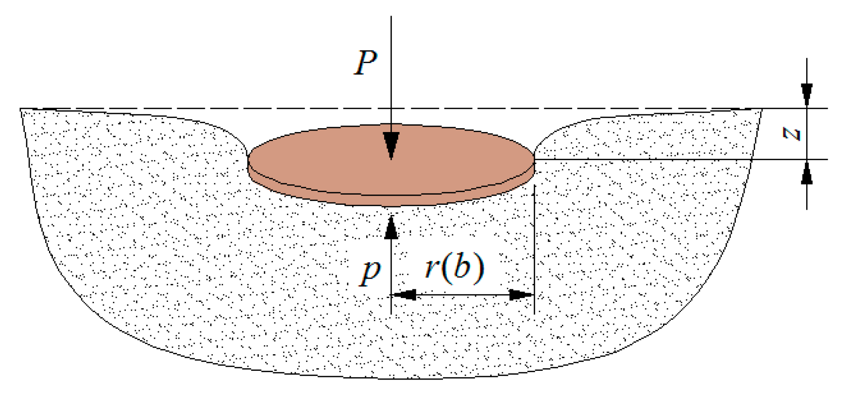
2.1. Bekker’s Pressure-Sinkage Theory

Under flat terrain conditions, the soil sinkage caused by the track shoe is related to the pressure-bearing characteristics of the soil [16]. The soil sinkage process is equivalent to that caused by a circular plate in the same environment, and the radius of the circular plate is equal to the width of the track shoe [8]. This principle is shown in Figure 2. In the figure, z is the soil sinkage, b is the width of the track shoe, r is the radius of the equivalent circular plate, P is the external force borne by the track shoe (circular plate), and p is the force borne by the unit area of the soil under the track shoe (circular plate), that is, the ground pressure.

According to Bekker’s study on the soil pressure-sinkage characteristics, the relationship between the ground pressure and the sinkage is expressed as follows:

$$p=\left(\frac{k_c}{b}+k_{\phi }\right)z^n$$

(1)

where k_c is the cohesive modulus (kN/mⁿ⁺¹); k_φ is the friction modulus (kN/mⁿ⁺²); n is the sinkage exponent.

From a theoretical viewpoint, it appears that there exists a linear relationship between the ground pressure and soil sinkage in the logarithmic coordinate system. Hence, the plate penetration test can be carried out with two circular plates with different radii. According to the test results, the soil sinkage parameters can be calculated using the least squares method in the logarithmic coordinate system [17].

For a specific HMT, the ground pressure is determined by the structural arrangement of the undercarriages and the HMT’s centroid position. When the soil’s sinkage parameters are known, the sinkage of the track shoe in the soil can be predicted using Equation (1) [18], and the driving resistance of the HMT can then be calculated according to the law of energy conservation [9,19].

2.2. Influence of Soil Water Content and Density on Pressure-Sinkage Characteristics

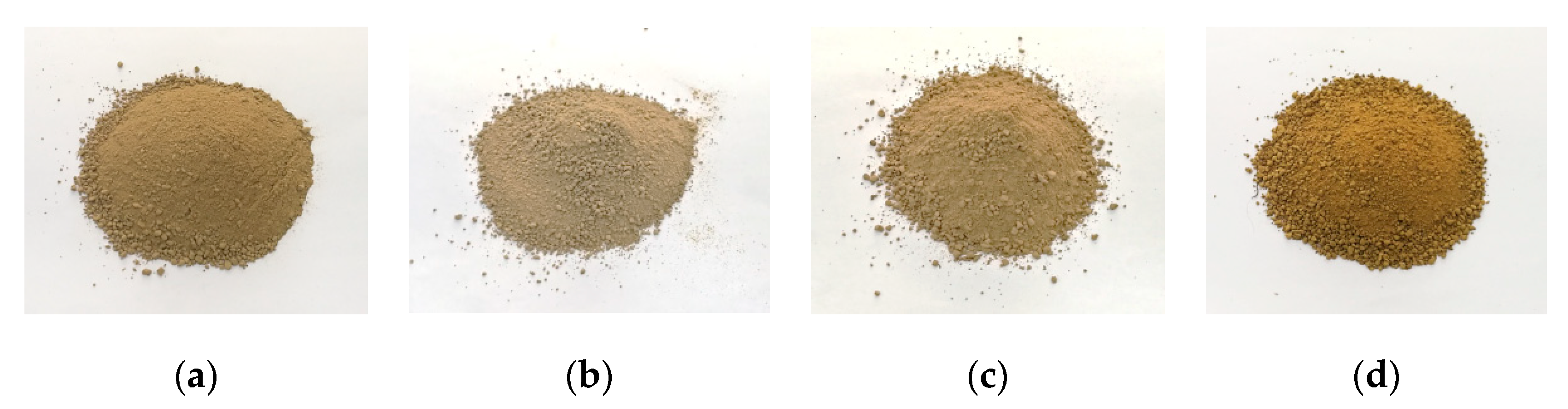
2.2.1. Soil Samples and Soil Type Determination

The four soil sample types used in this study were obtained from Yangling in Shaanxi Province (the sloping field test site in Northwest A&F University), Yangxian in Shaanxi Province (Qinba Mountain Area), and Huining and Jingning in Gansu Province (Loess Plateau Mountain Area), respectively. The air-dried states of the samples are shown in Figure 3.

The four abovementioned soil samples were numbered, and the MasterSizer 2000 laser particle analyzer (Malvern Panalytical Company, Cambridge, UK) was used to detect the particle size distribution. According to the international soil classification standards, soil samples can be classified according to their grain diameter [20]. The test and classification results are presented in

Table 1. Parameters of particle size distribution and classification of soil samples.

Place of Sampling	Sample No.	Content Percentage of Soil Particle Size (%)			Texture Grading
		Clay	Silt	Sand
		(d < 0.002)	(d = 0.002–0.02)	(d = 0.02–2)
Yangling, Shaanxi	1	31.82	35.58	32.60	Loamy clay
Yangxian, Shaanxi	2	38.49	33.67	27.84	Loamy clay
Huining, Gansu	3	23.11	30.78	46.11	Clay Loam
Jingning, Gansu	4	24.50	28.75	46.75	Clay loam

Note: d represents the soil particle diameter for all sizes (unit: mm).

.

Under different soil water contents, soil densities, grain compositions, and other conditions, the soil characteristics may greatly vary, and the water content exerts the most significant influence [5]. According to relevant data, a 3% change in the soil water content can cause great changes in the soil characteristics [21]. However, when HMTs travel on farming terrain, the sinkage of the track is often affected by the soil’s compactness, which mainly depends on the soil water content and bulk density [22]. Therefore, the influence of the soil water content and bulk density on the pressure–sinkage characteristics was first verified under flat ground conditions.

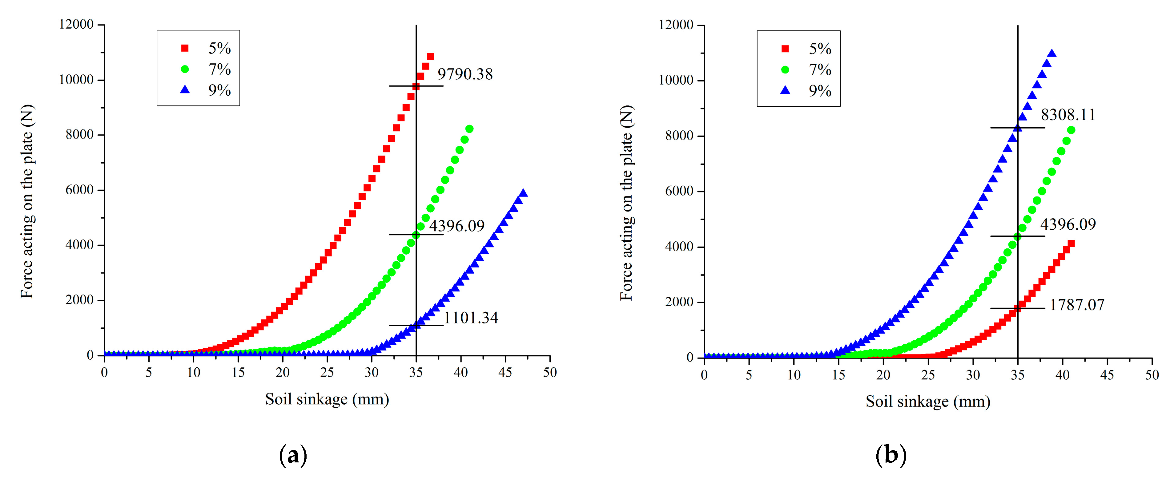
2.2.2. Influence of Soil Water Content and Bulk Density on Pressure-Sinkage Curve

• Soil water content and bulk density test

Let us consider soil sample No. 1 from Yangling, Shaanxi Province, as an example. The sample was collected at the depth range of 0–30 cm, the density was calculated, and the soil water content of the sample was measured. The results are presented in

Table 2. Soil water content and bulk density.

Depth of Sampling (cm)	Sample No.	Average Soil Water Content (%)	Average Density (mg·m−3)
0–10	5	5.6	1.84
10–20	5	7.1	2.26
20–30	5	7.9	1.98

.

As presented in Table 2, the mean values of the soil water content and bulk density at the depth of 0–30 cm were 6.9% and 2.03 mg·m⁻³, respectively. Therefore, a soil water content of 5%, 7%, and 9%, and bulk density of 1.5, 2.0, and 2.5 mg·m⁻³, were set to prepare the soil samples for plate penetration testing.

According to Chinese standard GB/T 50123-2019, the soil sample was placed at a ventilated spot for drying until it could be crushed. Then, the sample was filtered using a 5 mm bore diameter sieve to remove impurities. Finally, the sample was milled and thoroughly stirred, and the air-dried soil water content was determined.

Sufficient amounts of soil with soil water content of 5%, 7%, and 9% were prepared, respectively. The amounts of water required for the preparation were calculated as follows:

$$m_w=\frac{m_0}{1+0.01w_0}\times 0.01\left(w_1-w_0\right)$$

(2)

where m_w is the mass of the water required for the preparation (kg); m₀ is the mass of the air-dried soil (kg); w₀ is the soil water content of the air-dried soil (%); w₁ is the required soil water content of the sample (%).

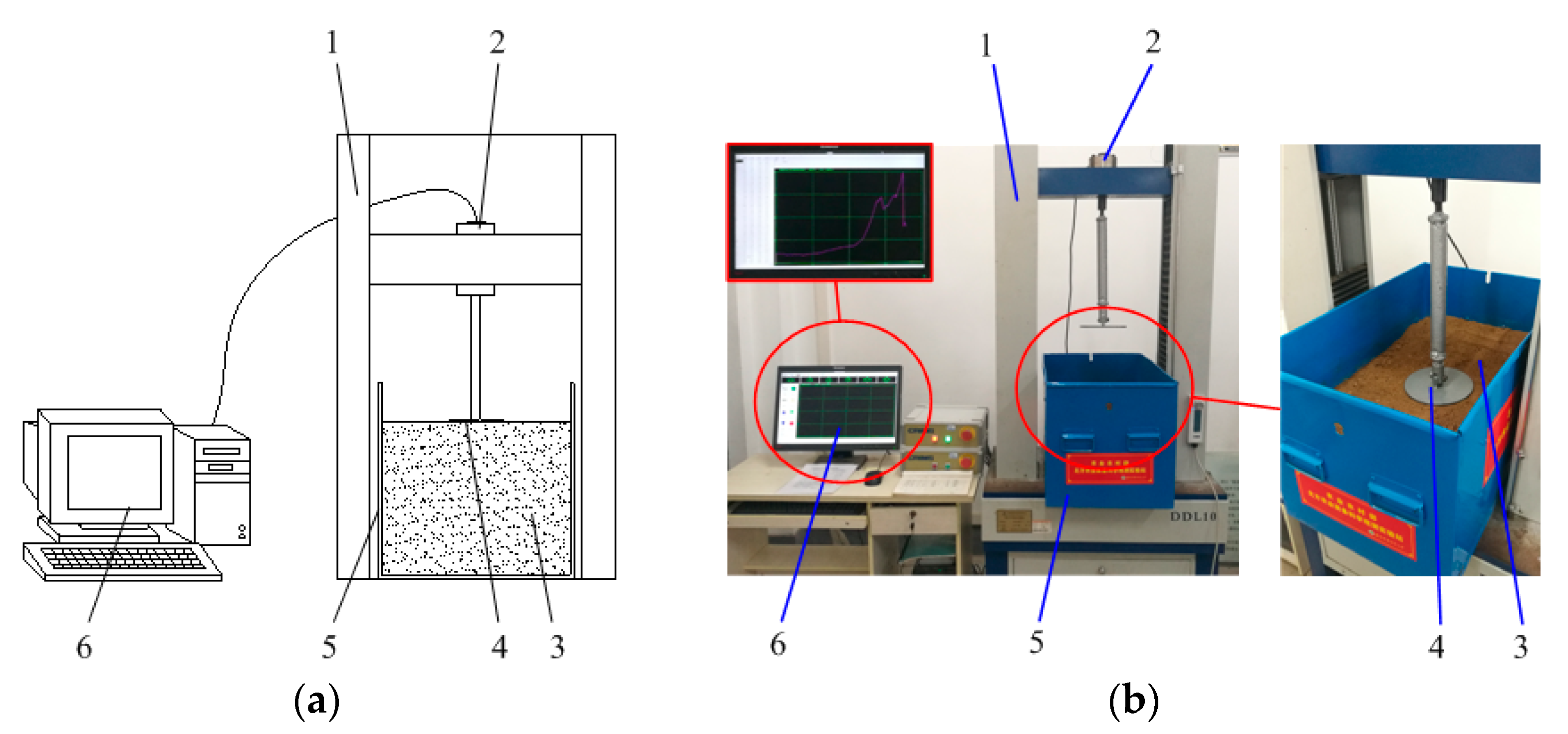
• Plate penetration test under flat terrain conditions

Before the test, the soil was compacted to the target bulk density. According to the classic plate penetration test method [8], a circular plate with radius of 80 mm was used in this test to compact the soil. The equipment used in the test is listed in

Table 3. Pressure–sinkage test equipment under sloped conditions.

Type	Name	Specification
Pressurized equipment and devices	DDL10 testing machine	Range < 10 kN
	No. 1 circular plate	Radius of 80 mm
	No. 2 circular plate	Radius of 100 mm
Soil tank		Length × width × height = 650 × 400 × 400 mm
Angle measuring device	Inclinometer
Soil preparation tools	Shovel, scrape board
Soil water content measuring equipment	Soil moisture meter	TZS-2X-G

. The test principle and system composition are shown in Figure 4a,b, respectively.

The plate penetration test was carried out under flat terrain conditions, and the relationship between the pressure and the soil sinkage is shown in Figure 5. As can be seen, with different soil water contents or densities, different curves were obtained. Under a bulk density of 2 mg·m⁻³, as the soil water content increased from 5% to 7% and 9%, the pressure increased 2.99 times and 7.89 times, respectively, when the soil sinkage was 35 mm. Under a soil water content of 7%, as the density increased from 1.5 mg·m⁻³ to 2.0 mg·m⁻³ and 2.5 mg·m⁻³, the pressure increased by 1.46 times and 3.65 times, respectively, when the soil sinkage was 35 mm. Therefore, it is concluded that the soil water content and density exert a certain influence on the sinkage process of the track shoe. Therefore, when investigating the vertical load-deformation relationship of soil under sloped terrain conditions, the slope angle should be considered as an important index affecting the soil sinkage, but the influence of the soil water content and bulk density on the test results should also be fully considered.

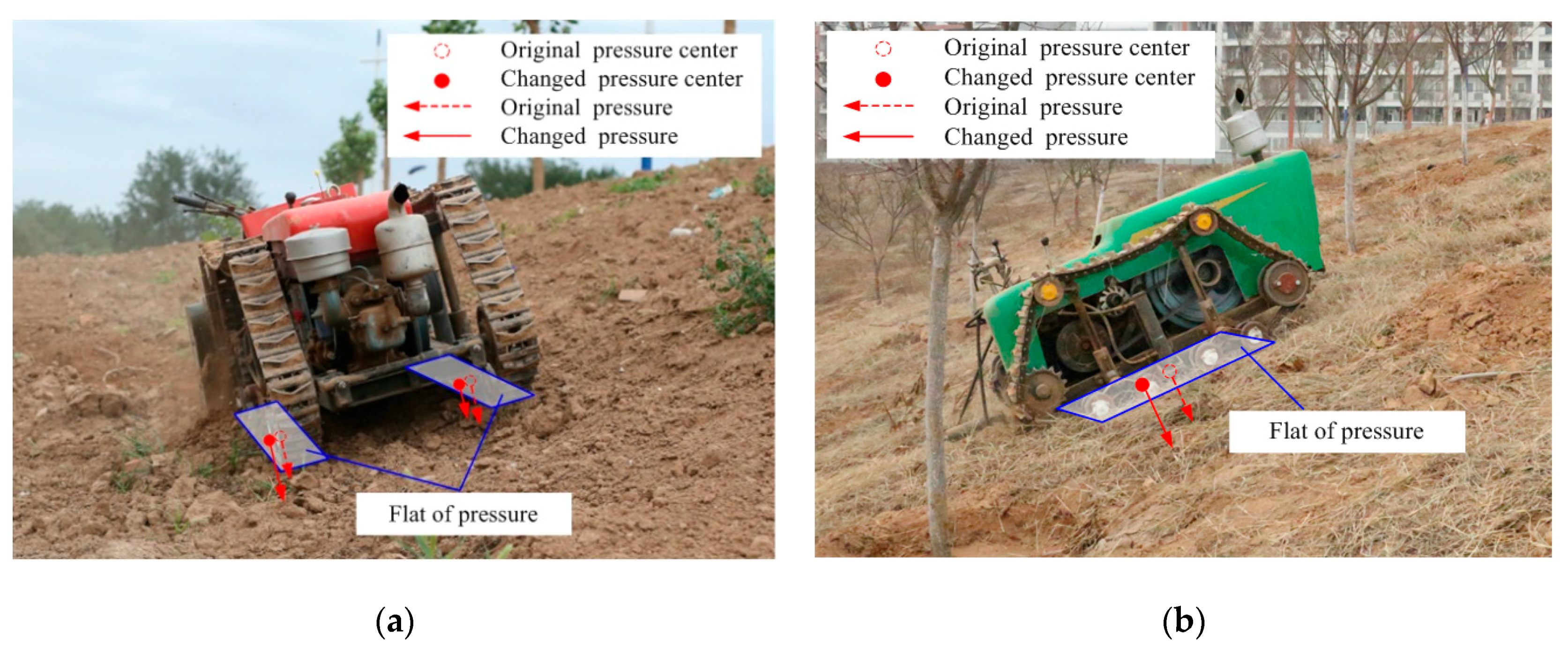
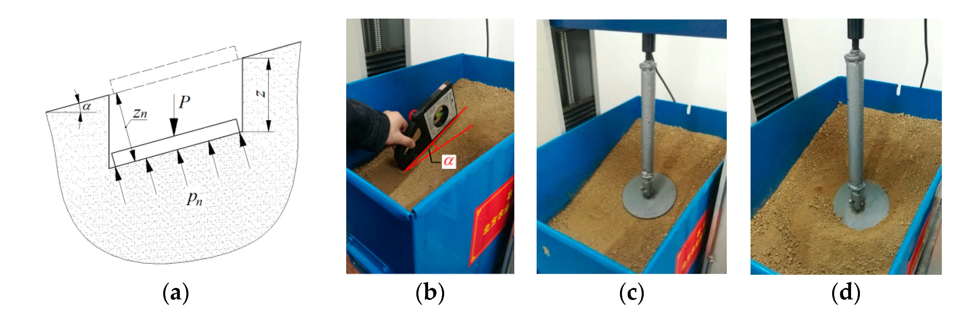
2.3. Modification of Bekker’s Model under Sloped Terrain Conditions

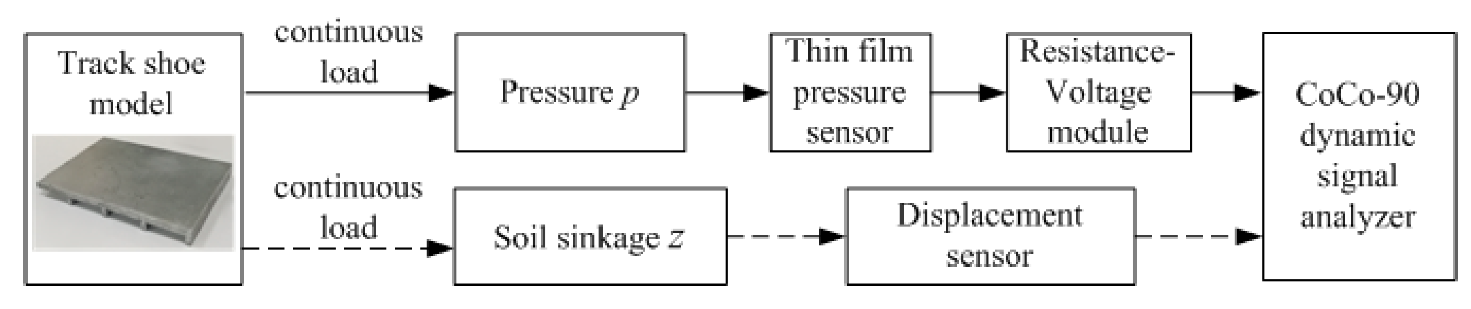
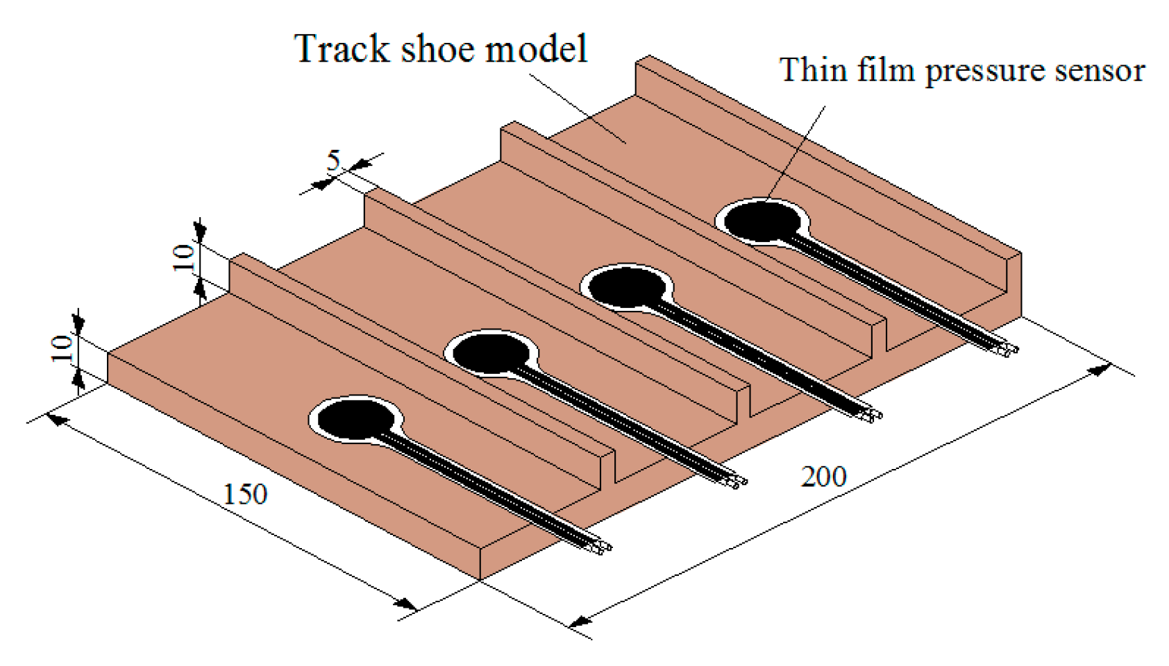
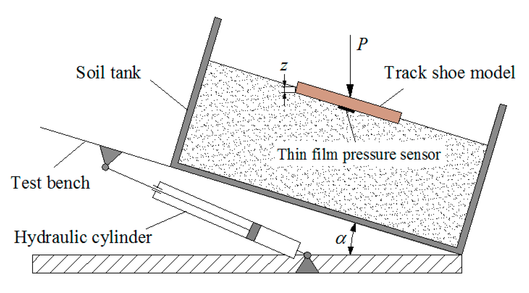
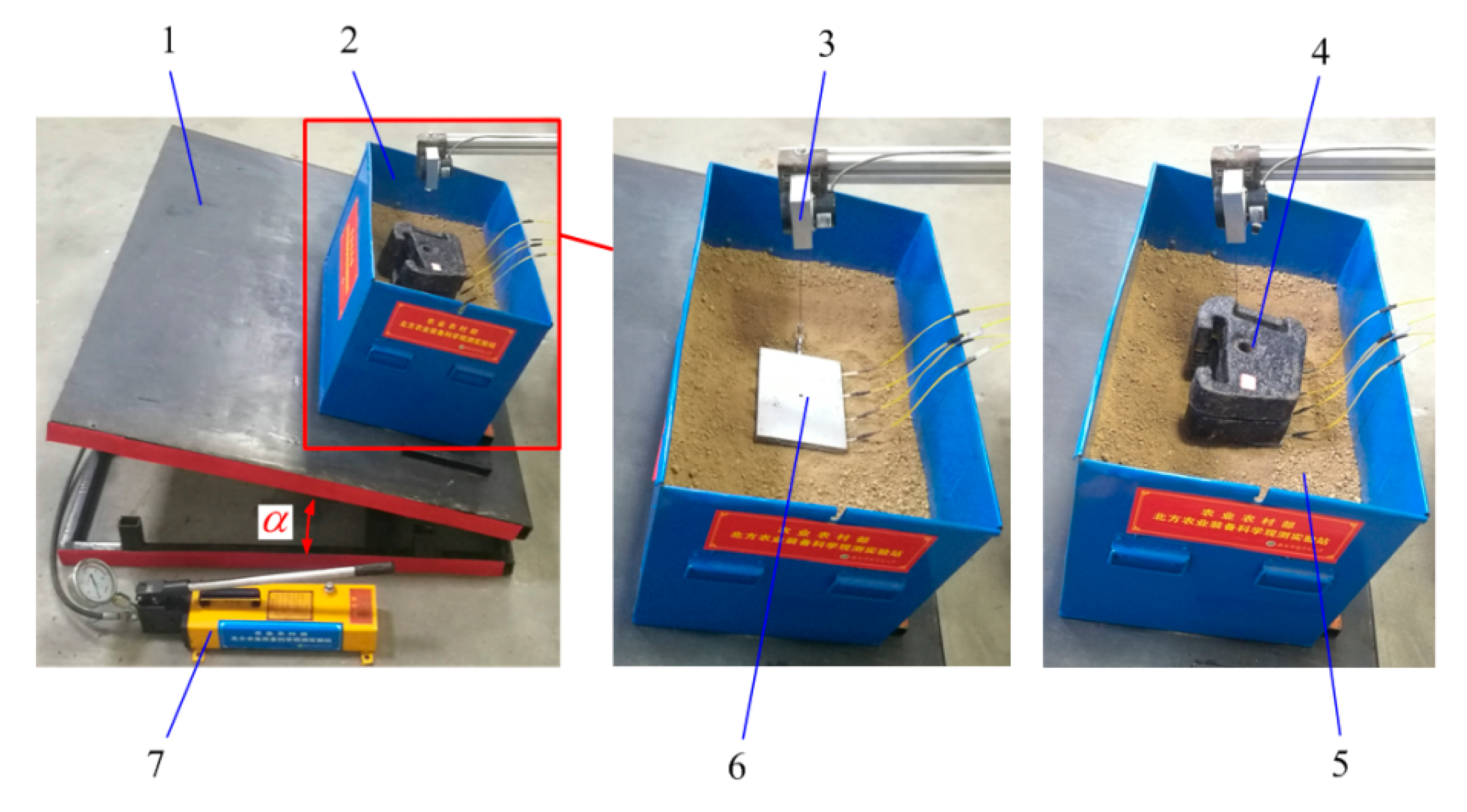
2.3.1. Test Scheme and Principle

In Bekker’s model, the sinkage parameters can be calculated from the pressure–sinkage curve. Therefore, the soil water content, bulk density, and slope angle were selected as the test factors, and the quadratic rotation orthogonal combination test was carried out to obtain the sinkage parameters of the four soil types.

Because the plastic limit of agricultural soil does not typically exceed 16% [23], 4% and 16% were considered as the lower and upper limits of the soil water content, respectively. According to the abovementioned bulk density measurement results, the bulk density at the depth range of 0–30 cm is 1.84 mg·m⁻³ at minimum and 2.26 mg·m⁻³ at maximum. Therefore, 1.5 mg·m⁻³ and 2.5 mg·m⁻³ were considered as the lower and upper limits of the bulk density. Because a farmland slope greater than 20° will cause severe soil erosion [24], 0°–20° was considered as the range of the slope angle in this study. The horizontal encoding of each factor is listed in

Table 4. Factors and levels of test.

Encoding	Factors
	Soil Water Content X1 (%)	Bulk Density X2 (mg·m−3)	Slope Angle X3 (°)
−1.682	4.0	1.5	0
−1	6.4	1.7	4
0	10.0	2.0	10
1	13.6	2.3	16
1.682	16.0	2.5	20

.

The plate penetration test under flat terrain conditions was considered in the test, and plates were used to simulate the track shoe of the HMT. Figure 6a shows the forces exerted when the plates were initially pressed into the soil under sloped terrain conditions. In the figure, z is the soil sinkage, and p_n is the reactive pressure in the direction perpendicular to the plate. As shown in Figure 6b, the slope angle was measured with an inclinometer before the test, and circular plates with a radius of 80 mm and 100 mm were subsequently applied to press the soil sample at constant speed. The condition of the soil before and after pressing is shown in Figure 6c,d, respectively.

2.3.2. Calculation of Soil Sinkage Parameters

Let us consider the No. 1 Yangling soil sample as an example. The effective pressure–sinkage relationship curve collected under the actual soil water content of 4.0%, slope angle of 0°, and density of 1.5 mg·m⁻³ is shown in Figure 7.

The force data were converted into the pressure, and the sinkage parameters were calculated using the least squares method [25], as follows:

$$\{\begin{array}{l}{n}_m=\frac{{\displaystyle \sum w_r{\displaystyle \sum w_r\ln p_i\ln z_i-{\displaystyle \sum w_r\ln p_i{\displaystyle \sum w_r\ln z_i}}}}}{{\displaystyle \sum w_r{\displaystyle \sum w_r{\left(\ln z_i\right)}^2-{\left({\displaystyle \sum w_r\ln z_i}\right)}^2}}}\\ K_m=k_c/b+k_{\phi }=\exp \frac{{\displaystyle \sum w_r\ln p_i-n{\displaystyle \sum w_r\ln z_i}}}{{\displaystyle \sum w_r}}\end{array}$$

(3)

where n_m is the sinkage exponent obtained by calculating the No. m effective curve; K_m is the equivalent modulus of deformation obtained by calculating the No. m effective curve (kN/mⁿ⁺²); w_r is the weight factor (because each test was independent and without repetition, so the weight is equal to one); p_i is the pressure obtained in each test (kPa); z_i is the sinkage obtained for each sample (m).

The sinkage exponent n and equivalent deformation modulus K can be obtained as follows:

$$\{\begin{array}{l}n=\frac{{\displaystyle \sum n_m}}{m}\\ K=\frac{{\displaystyle \sum K_m}}{m}\end{array}$$

(4)

The cohesive modulus k_c and the frictional modulus k_φ can be obtained as follows:

$$\{\begin{array}{l}{k}_c=\frac{K_{b=b_1}-K_{b=b_2}}{b_2-b_1}{b}_1{b}_2\\ k_{\phi }=\frac{b_1{K}_{b=b_1}-b_2{K}_{b=b_2}}{b_1-b_2}\end{array}$$

(5)

where, K_b=b1 and K_b=b2 are the equivalent modulus of the soil deformation measured by two circular plates, respectively (kN/mⁿ⁺²); b₁ and b₂ denote the radii of the two circular plates, respectively (m).

The sinkage parameters corresponding to different test numbers are listed in

Table 5. Results of soil sinkage parameter calculation.

Test No.	Soil Water Content X1	Bulk Density X2	Slope Angle X3	Sinkage Exponent Y1	Cohesive Modulus Y2	Friction Modulus Y3
1	−1	−1	−1	1.3748	324	9406
2	1	−1	−1	1.4824	382	12,084
3	−1	1	−1	1.5059	468	9573
4	1	1	−1	1.6628	528	12,658
5	−1	−1	1	1.8626	673	5528
6	1	−1	1	1.8359	752	9016
7	−1	1	1	1.8191	780	6023
8	1	1	1	1.7628	816	12,420
9	−1.682	0	0	1.5703	228	6429
10	1.682	0	0	1.6425	318	13,029
11	0	−1.682	0	1.6686	809	9560
12	0	1.682	0	1.7028	998	10,516
13	0	0	−1.682	1.4064	436	11,806
14	0	0	1.682	1.9217	984	6487
15	0	0	0	1.7259	1298	10,131
16	0	0	0	1.7262	1305	10,052
17	0	0	0	1.7301	1310	10,198
18	0	0	0	1.7108	1296	9972
19	0	0	0	1.6991	1308	11,007
20	0	0	0	1.6311	1311	10,155
21	0	0	0	1.6925	1296	10,239
22	0	0	0	1.7096	1303	9980
23	0	0	0	1.7305	1295	10,054

.

Multiple regression fitting was carried out on the data presented in

Table 6. Analysis of variance.

Variance	Sinkage Exponent				Cohesive Modulus				Friction Modulus
	Quadratic Sum	Degree of Freedom	F	p	Quadratic Sum	Degree of Freedom	F	p	Quadratic Sum	Degree of Freedom	F	p
Model	0.400	9	57.30	<0.01 ***	3.50 × 106	9	7945.82	<0.01 ***	9.11 × 107	9	63.66	<0.01 ***
X1	6.72 × 10−3	1	8.71	0.0112 **	10817.55	1	221.17	<0.01 ***	5.23 × 107	1	329.53	<0.01 ***
X2	4.6 × 10−3	1	6.05	0.0287 **	44418.80	1	908.14	<0.01 ***	2.85 × 106	1	17.98	<0.01 ***
X3	0.330	1	427.06	<0.01 ***	3.68 × 105	1	7515.79	<0.01 ***	2.84 × 107	1	178.38	<0.01 ***
X1 × 2	4.85 × 10−5	1	0.063	0.8059	210.13	1	4.30	0.0586 *	1.37 × 106	1	8.65	0.0115 **
X1X3	0.015	1	19.57	<0.01 ***	1.13	1	0.023	0.8818	2.12 × 106	1	13.36	<0.01 ***
X2X3	0.023	1	29.70	<0.01 ***	1770.13	1	36.19	<0.01 ***	1.25 × 106	1	7.84	0.015 **
$X_1^2$	0.017	1	21.45	<0.01 ***	2.10 × 106	1	42916.14	<0.01 ***	4.55 × 105	1	2.86	0.1145
$X_2^2$	2.85 × 10−4	1	0.37	0.5536	3.14 × 105	1	6417.35	<0.01 ***	57162.63	1	0.36	0.5591
$X_3^2$	2.25 × 10−3	1	2.91	0.1117	3.94 × 105	1	14185.06	<0.01 ***	2.24 × 106	1	14.07	<0.01 ***
Residual error	0.01	13			635.85	13			2.07 × 106	13
Lack of fit	2.17 × 10−3	5	0.44	0.8086	309.63	5	1.52	0.2851	1.26 × 106	5	2.52	0.1181
Error	7.86 × 10−3	8			326.22	8			8.03 × 105	8
Sum	0.410	22				22			9.31 × 107	22

Significance level at * p ≤ 0.1; ** p ≤ 0.05; *** p ≤ 0.01.

using the Design-Expert 8.0.6 software, and the regression equations of the sinkage exponent Y₁, cohesive modulus Y₂, and frictional modulus Y₃ were obtained. The analysis of variance is presented in Table 6.

As can be seen, the overall model of the test is extremely significant, whereas the result obtained by the lack of fit test is not significant. This indicates that the test is effective. According to the P value of each factor, the non-significant factors were eliminated to obtain the regression equation of each index.

Equation (6) reflects the functional relationship between the sinkage parameters of Yangling loamy clay and the soil water content, bulk density, and slope angle. Similarly, the regression equation of the sinkage parameters of soil samples No. 2–4 can be obtained as expressed by Equations (7)–(9).

$$\{\begin{array}{ll}{Y}_1=n(w,\rho ,\alpha )=& 0.015+0.073w+0.533\rho +0.114\alpha -0.002w\alpha -0.03\rho \alpha -0.003w^2\\ Y_2=k_c(w,\rho ,\alpha )=& -9510.021+588.86w+6684.854\rho +162.805\alpha -4.832w\rho \\ & -8.415\rho \alpha -28.557w^2-1590.14{\rho }^2-5.91{\alpha }^2\\ Y_3=k_{\varphi }(w,\rho ,\alpha )=& 13660.843-209.581w-1887.838\rho -719.616\alpha \\ & +390.794w\rho +24.289w\alpha +223.304\rho \alpha -10.612{\alpha }^2\end{array}$$

(6)

$$\{\begin{array}{ll}{Y}_1=n(w,\rho ,\alpha )=& 0.176+0.061w+0.336\rho +0.109\alpha -0.002w\alpha -0.029\rho \alpha -0.002w^2\\ Y_2=k_c(w,\rho ,\alpha )=& -10041.498+580.335w+7167.464\rho +166.553\alpha -12.728w\rho \\ & -10.041\rho \alpha -27.575w^2-1686.825{\rho }^2-6.072{\alpha }^2\\ Y_3=k_{\varphi }(w,\rho ,\alpha )=& 16232.556-142.722w-5773.781\rho -831.203\alpha \\ & +273.415w\rho +18.408w\alpha +289.065\rho \alpha -8.353{\alpha }^2\end{array}$$

(7)

$$\{\begin{array}{ll}{Y}_1=n(w,\rho ,\alpha )=& 0.490+0.083\alpha -0.002w\alpha -0.024\rho \alpha -0.002w^2\\ Y_2=k_c(w,\rho ,\alpha )=& -8827.736+580.699w+6479.259\rho +140.080\alpha \\ & -28.207w^2-1539.777{\rho }^2-4.784{\alpha }^2\\ Y_3=k_{\varphi }(w,\rho ,\alpha )=& 13043.375+355.806w+356.097\rho -794.321\alpha \\ & +28.414w\alpha +244.518\rho \alpha -31.434w^2-11.141{\alpha }^2\end{array}$$

(8)

$$\{\begin{array}{ll}{Y}_1=n(w,\rho ,\alpha )=& 0.421+0.08\alpha -0.002w\alpha -0.023\rho \alpha -0.003w^2\\ Y_2=k_c(w,\rho ,\alpha )=& -9178.975+606.066w+6815.484\rho +149.641\alpha \\ & -28.954w^2-1607.348{\rho }^2-4.978{\alpha }^2\\ Y_3=k_{\varphi }(w,\rho ,\alpha )=& 19563.312+244.659w-2754.647\rho -1142.649\alpha \\ & +26.452w\alpha +403.687\rho \alpha -28.751w^2-10.131{\alpha }^2\end{array}$$

(9)

From the above equations, it can be seen that the regression equations of the sinkage parameters of loamy clay (Soils No. 1 and 2) and clay loam (Soils No. 3 and 4) have different terms. The regression equations of the same soil type have the same terms, and the coefficients are similar. Therefore, we can determine whether different soils belong to the same area by comparing the terms and coefficients of the regression equation of the soil sinkage parameters.

By substituting Equations (6)–(9) into Bekker’s model, the sinkage model of sloped terrain can be obtained as follows:

$$p=\left(\frac{Y_2}{b}+Y_3\right)z^{Y_1}=\left(\frac{k_c(w,\rho ,\alpha )}{b}+k_{\varphi }(w,\rho ,\alpha )\right)z^{n(w,\rho ,\alpha )}$$

(10)

3. Results and Discussion

In this study, the effectiveness of the abovementioned model (Equation (10)) was verified using a track shoe model under the static conditions and a prototype HMT under dynamic conditions.

3.1. Static Test of Track Shoe Model

The measured values of the thin-film pressure sensor were obtained under soil water contents of 10%, bulk density of 2 mg·m⁻³, and slope angle of 10°, respectively. Then, the obtained values were compared to the values calculated using Equation (10) to verify the effectiveness of the modified model under static conditions.

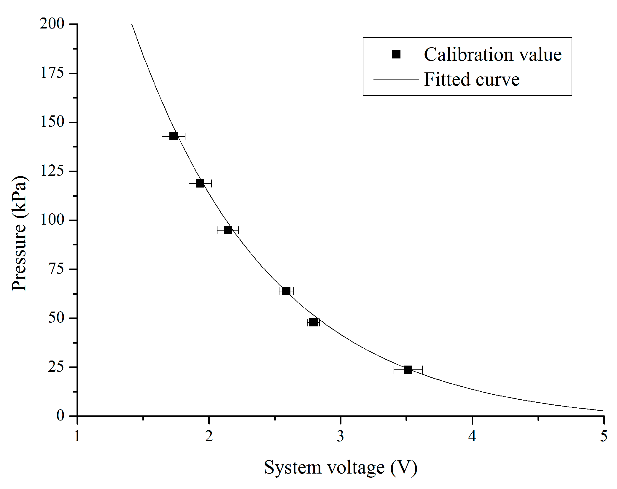
3.1.1. Sensor Calibration

Before the effectiveness verification of the modified model, the IMS-C20A thin-film pressure sensor (Figure 8) was calibrated, and the relationship between the sensor pressure and the voltage was established.

Different block masses were used to apply continuous vertical loads to the sensor, and a voltage-resistance conversion module was used to convert the resistance into voltage. The data were read and recorded by a dynamic signal analyzer (Figure 9).

Calibration was carried out for 10 groups to obtain the average values, which are presented in

Table 7. System output voltage under different loads (unit: V).

	No.	Vertical Load/kg
		0.761	1.533	2.045	3.045	3.806	4.578
Output voltage	1	3.926	3.102	2.715	2.210	1.962	1.789
	2	3.728	3.025	2.642	2.259	1.926	1.718
	3	3.696	3.067	2.583	2.108	1.980	1.733
	4	3.936	3.150	2.722	2.236	2.011	1.847
	5	4.039	3.100	2.738	2.304	2.056	1.894
	6	3.986	3.152	2.684	2.209	1.989	1.793
	7	3.864	3.087	2.748	2.211	2.027	1.881
	8	3.921	3.137	2.868	2.214	2.033	1.834
	9	4.024	2.983	2.726	2.307	2.065	1.799
	10	3.904	3.163	2.798	2.375	2.063	1.895
Mean value		3.902	3.097	2.722	2.243	2.011	1.818
Standard deviation		0.108	0.056	0.074	0.069	0.044	0.060

.

The vertical load can be converted into sensor pressure by calculation, and fitting was carried out using the Origin 8.6 software. The result is expressed by Equation (11).

$$p_c=751.87e^{\frac{-U}{1.063}}-4.256$$

(11)

The determination coefficient of Equation (11) is 0.998, which indicates that the sensor pressure has a good exponential relationship with the system’s voltage, as shown in Figure 10. Hence, Equation (11) can be used to verify the effectiveness of the modified model.

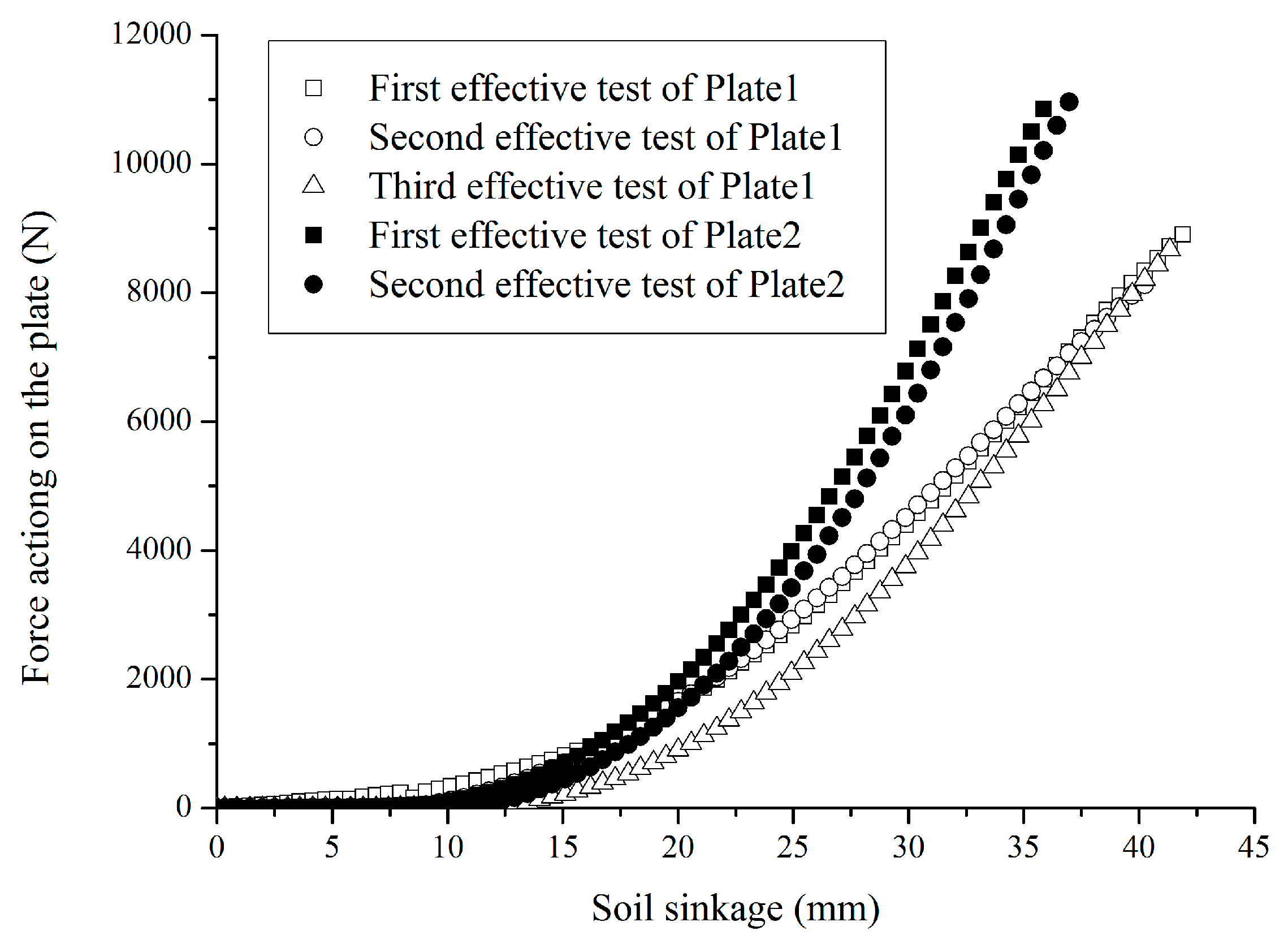
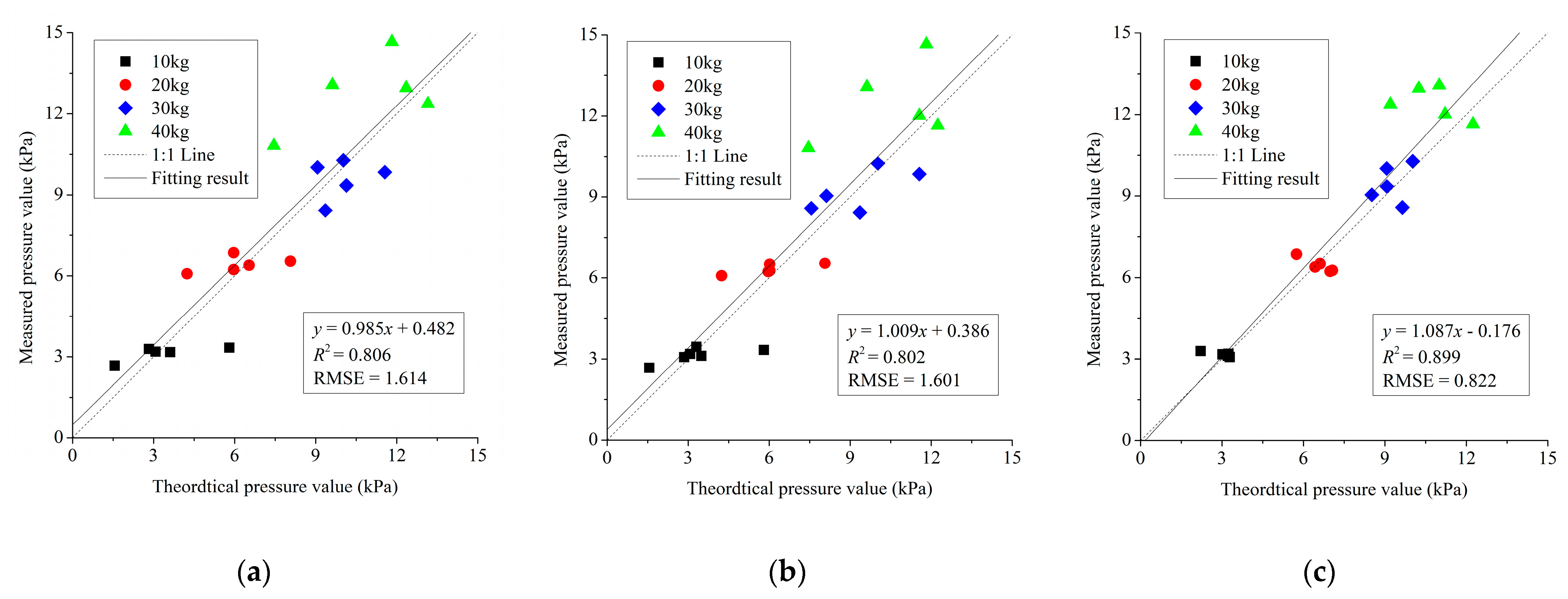
3.1.2. Verification Test of Track Shoe Model

The test process is shown in Figure 11.

Before the test, four thin-film pressure sensors were attached to the back of the track shoe model (Figure 12), and the track shoe model was placed in the soil tank. According to the testing process, intermediate-level values (soil water content of 10%, bulk density of 2 mg·m⁻³, and slope angle of 10°) were selected to carry out the verification test, and twenty pressure groups were measured under each condition. The principle of the verification test is shown in Figure 13; the status of the track shoe model placed in the soil tank is shown in Figure 14.

Weights with a mass of 10–40 kg were used to apply force to the track shoe model, and the slope angle could be changed through a test bench. The system composition is shown in Figure 15.

Figure 16 shows the test results of the No. 1 soil sample. As can be seen, when the soil water content was 10%, the bulk density was 2 mg·m⁻³ and the slope angle was 10°. The pressure calculated by Equation (10) is relatively close to the results measured by the thin-film pressure sensor, and the root-mean-square errors are 1.614, 1.601, and 0.822. The main reason is that the modified model was established by considering that the forces are uniformly distributed on the interaction surface between the track shoe model and the soil. However, under actual conditions, owing to the discrete and uneven distribution of soil, the pressure distributed at the bottom of the track shoe model is not completely even.

The test results reveal that on the basis of a certain dimension parameters of the track shoe model, Equation (10) can satisfactorily reflect the soil pressure–sinkage characteristic with different soil water contents, bulk densities, and slope angles, under static conditions. It has a certain guiding significance for the precise calculation of the soil sinkage parameters, and can provide a data foundation for the static analysis of HMTs under hillside terrain conditions.

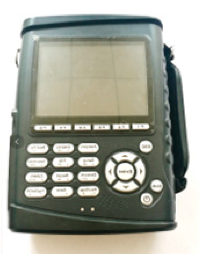
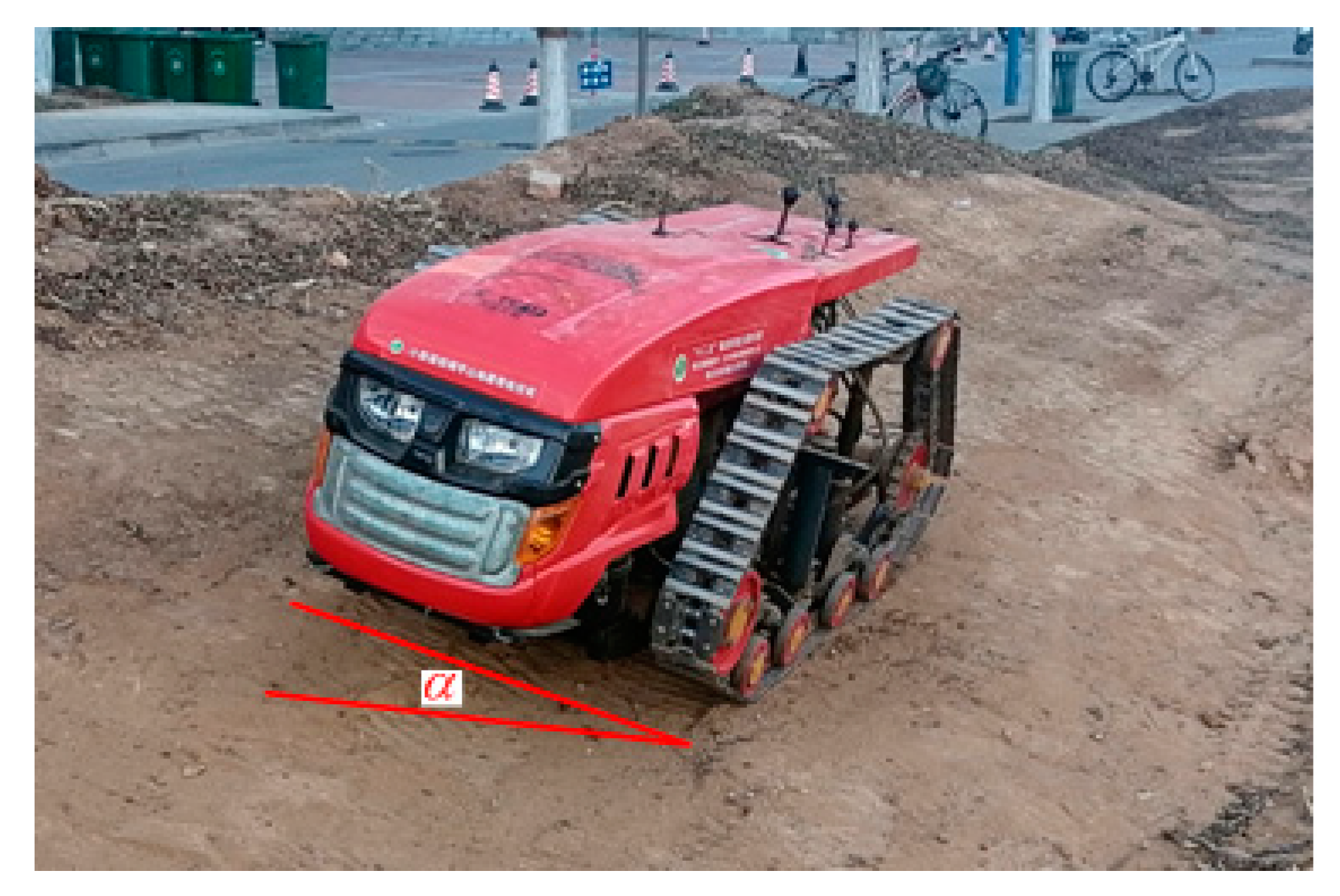
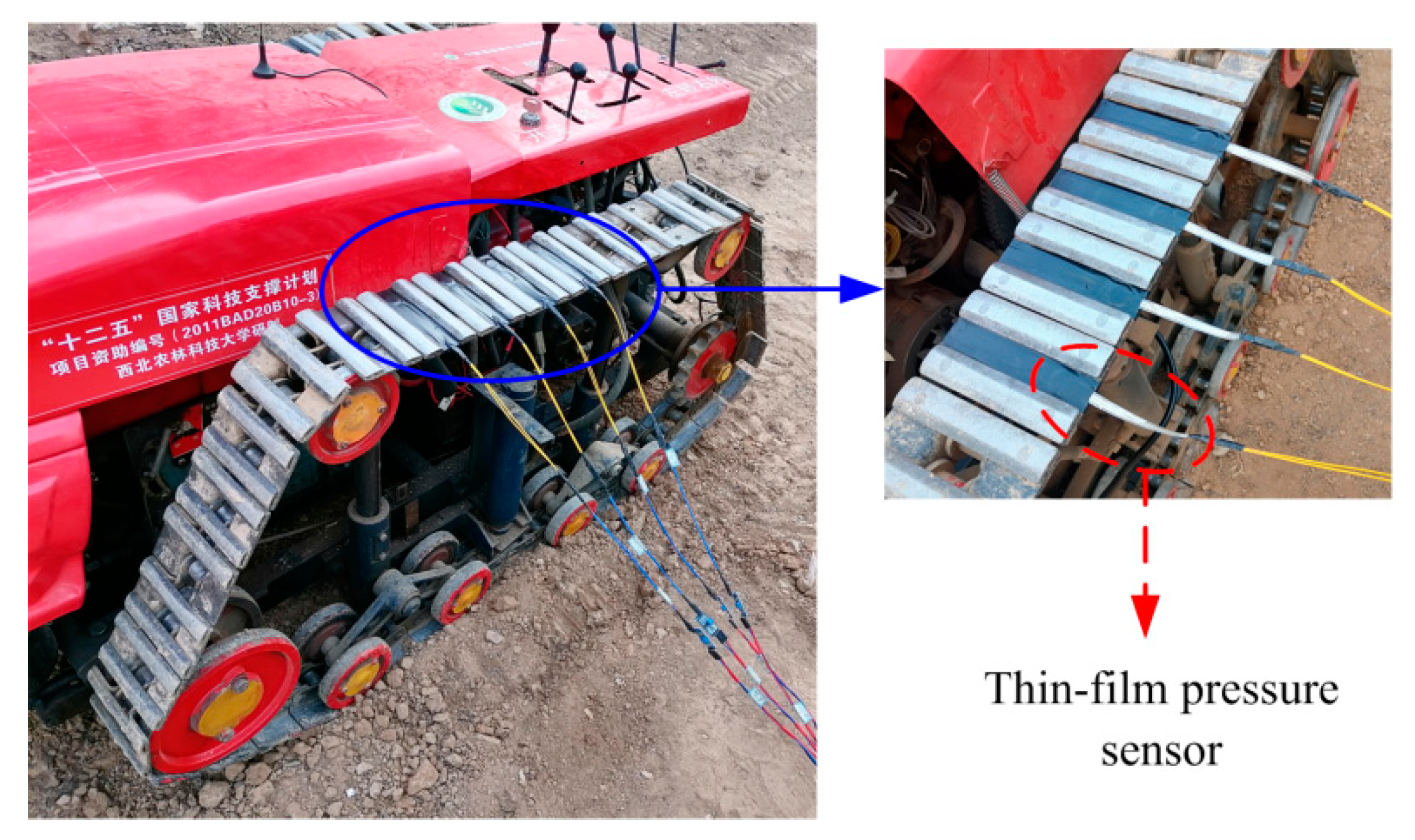
3.2. Dynamic Pressure Test of HMT Prototype

A 3D scanner was used to reconstruct the surface appearance of the soil so as to obtain the initial rut depth under three random soil water content, bulk density, and slope angle conditions. The pressure value was calculated using Equation (10). Then, the pressure under both sides of the track of the HMT prototype was measured by driving the prototype along the contour line on a slope to verify the effectiveness of the modified model under dynamic conditions.

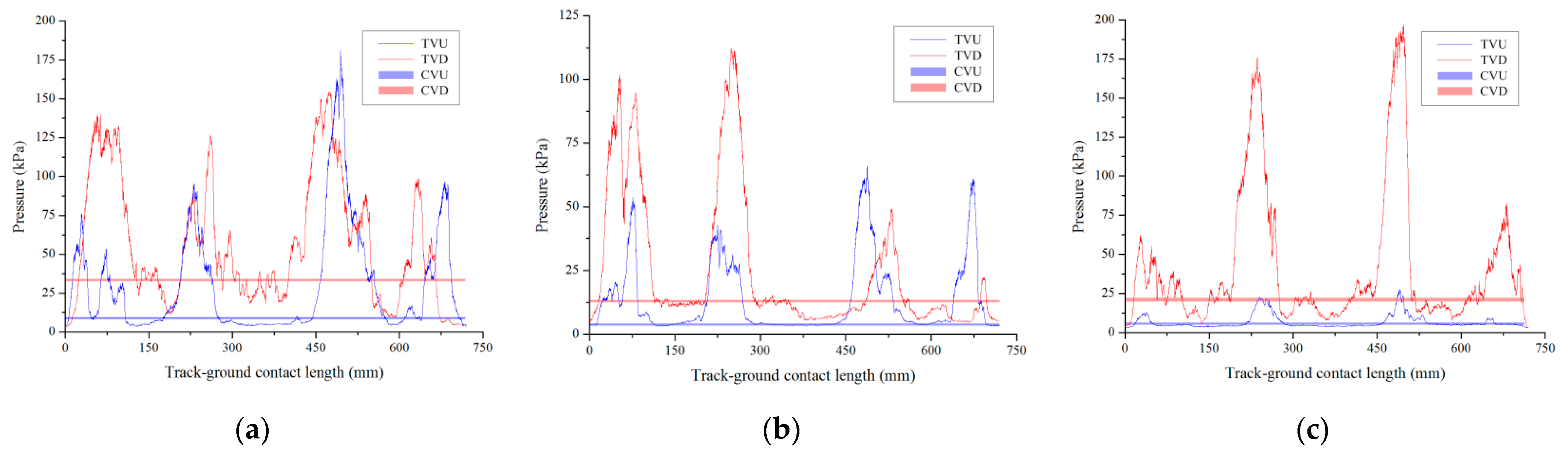
3.2.1. Pressure Test

The HMT prototype is shown in Figure 17; its ground pressure on the horizontal surface was 34.84 kPa.

Four thin-film pressure sensors were attached to both sides of the track, as shown in Figure 18. Pressure data were collected and recorded by the Coco-90 dynamic signal analyzer.

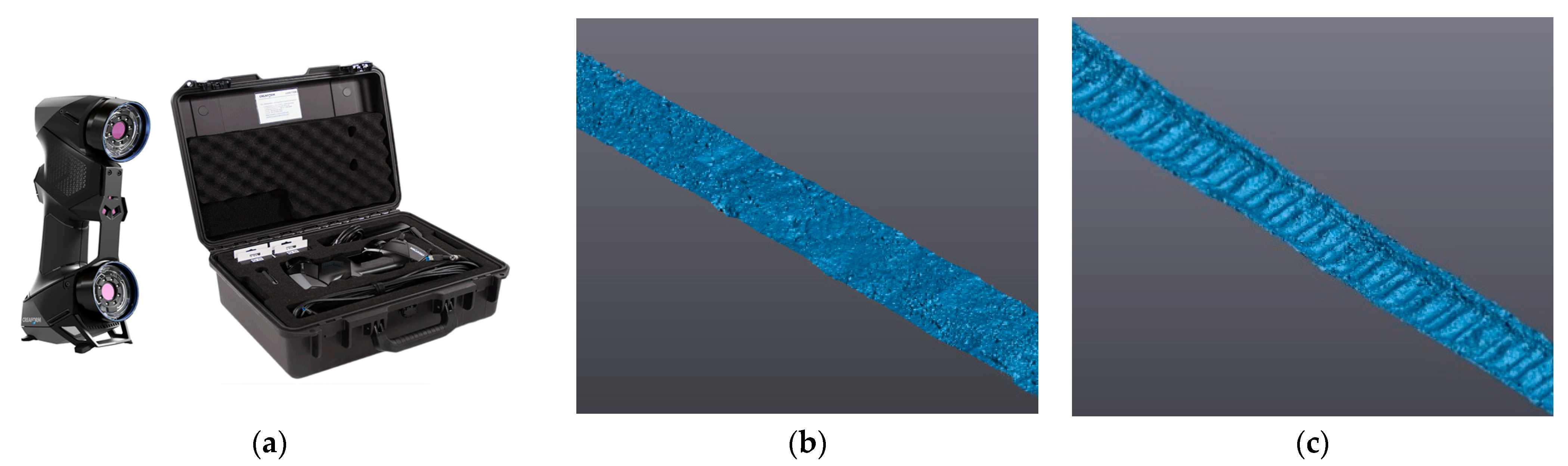
3.2.2. Measurement of Rut Depth

A 3D scanner (HandySCAN, Creaform, Lévis, QC, Canada) with a scanning accuracy of 0.5 mm was used to obtain the appearance of the sloped terrain’s surface, as shown in Figure 19. The rut depth of the entire track was obtained by calculating the difference between the two states of the sloped terrain’s surface appearance in the vertical direction.

Then, thirty groups of depth values between the four supporting wheels were measured for the subsequent calculation.

3.2.3. Analysis of Test Results

According to the measured depth values, Equation (10) was used to calculate the pressure of the two tracks under random soil conditions. The obtained values were 8.06 ± 0.11 kPa and 33.06 ± 0.86 kPa, 4.42 ± 0.23 kPa and 13.77 ± 0.23 kPa, and 5.99 ± 0.07 kPa and 19.35 ± 0.22 kPa. The results were compared with the measured values, as shown in Figure 20.

As can be seen from the figure, the measured values of the two sides of the track (TVU and TVD in the figure) can obviously reflect the change of the pressure distributed under the track. The pressure of the lower track is significantly greater than the pressure of the upper track between the supporting wheels. Although the measured values (CVU and CVD in the figure) have a significant variation range, they are essentially consistent with the calculated values between the supporting wheels.

By comparison, it can be seen that on the basis of a certain track’s parameters, the pressure calculated by Equation (10) essentially reflects the actual force of the track between the supporting wheels, but could not be used to calculate the actual force under the supporting wheels. Therefore, the proposed modified soil pressure–sinkage model could only provide a theoretical foundation for the analysis of the force between the supporting wheels, when HMTs are subjected to dynamic conditions.

4. Conclusions

With the objective of overcoming the limitations of Bekker’s soil pressure–sinkage model, the influence of different soil water contents and soil densities on the soil’s pressure and sinkage relationship was verified by considering flat terrain conditions. The results obtained by plate penetration testing reveal that, under different soil water contents and bulk densities, the pressure changes significantly when the sinkage is 35 mm. It indicates that the soil water content and bulk density exert a significant influence on the soil pressure–sinkage characteristics.

Based on the quadratic orthogonal rotating combination testing method, plate penetration tests were carried out under different soil water contents, soil densities, and slope angles. The soil sinkage parameters of Yangling, Yangxian, Huining, and Jingning were obtained. The analysis results obtained using the regression equation can provide a new approach for determining the dependency of different soils. The regression equations of the sinkage parameters were introduced into Bekker’s model to obtain the pressure-sinkage model of sloped terrain.

Under soil water content of 10%, bulk density of 2 mg·m⁻³, and slope angle of 10°, the proposed models were used to calculate the pressure based on a track shoe model. The calculated pressure values were compared with the measured values, and the root-mean-square error was found to be small, which is, 1.614, 1.601, and 0.822, respectively. The results obtained by dynamic testing under three random conditions revealed that the modified soil pressure–sinkage model can effectively calculate the force between the supporting wheels. It is significant for the arrangement of HMT undercarriages and driving resistance reduction under sloped terrain conditions.

References

1. Wang, Y.J.; Yang, F.Z.; Pan, G.T.; Liu, H.Y.; Liu, Z.J.; Zhang, J.Q. Design and testing of a small remote-control hillside tractor. Trans. ASABE 2014, 57, 363–370. [Google Scholar] [CrossRef]
2. Luoyang Tractor Research Institute, Ministry of Machinery and Electronics Industry, China. Tractor Design Manual, 1st ed.; China Machine Press: Beijing, China, 1994; Volume 1, p. 200. (In Chinese) [Google Scholar]
3. Zhang, Z.W.; Yang, F.Z.; Zhang, Z.P. Analysis on Driving Stability of Caterpillar Tractor on Ramp. Agric. Equip. Veh. Eng. 2010, 11, 7–10. (In Chinese) [Google Scholar] [CrossRef]
4. Evans, I. The sinkage of tracked vehicles on soft ground. J. Terramech. 1964, 1, 33–43. [Google Scholar] [CrossRef]
5. Uffelmann, F.L.; Evans, I. The performance of heavy tracked vehicles on soft cohesive soil. J. Terramech. 1965, 2, 33–45. [Google Scholar] [CrossRef]
6. Mason, G.L.; Salmon, J.E.; Mcleod, S.; Jayakumar, P.; Smith, W. An overview of methods to convert cone index to bevameter parameters. J. Terramech. 2020, 87, 1–9. [Google Scholar] [CrossRef]
7. Shaikh, S.A.; Li, Y.M.; Zheng, M.; Chandio, F.A.; Ahmad, F.; Tunio, M.H.; Abbas, I. Effect of grouser height on the tractive performance of single grouser shoe under different soil moisture contents in clay loam terrain. Sustainability 2021, 13, 1156. [Google Scholar] [CrossRef]
8. Bekker, M.G. Introduction to Terrain-Vehicle Systems; University of Michigan Press: Ann Arbor, MI, USA, 1969. [Google Scholar]
9. He, R.; Sandu, C.; Khan, S.K.; Guthrie, A.G.; Els, P.S.; Hamersma, H.A. Review of terramechanics models and their applicability to real-time applications. J. Terramech. 2019, 81, 3–22. [Google Scholar] [CrossRef] [Green Version]
10. Yang, C.B.; Yang, G.; Liu, Z.F.; Chen, H.X.; Zhao, Y.S. A method for deducing pressure-sinkage of tracked vehicle in rough terrain considering moisture and sinkage speed. J. Terramech. 2018, 79, 99–113. [Google Scholar] [CrossRef]
11. Reece, A.R. Principles of soil-vehicle mechanics. Proc. Inst. Mech. Eng. Automob. Div. Part 2A 1965, 180, 45–67. [Google Scholar] [CrossRef]
12. Onafeko, O.; Reece, A.R. Soil stresses and deformations beneath rigid wheels. J. Terramech. 1967, 4, 59–80. [Google Scholar] [CrossRef]
13. Ageikin, J.S. Off-the-Road Wheeled and Combined Traction Devices: Theory and Calculation; Amerind Publishing Company: New Delhi, India, 1987. [Google Scholar]
14. Lyasko, M. LSA model for sinkage predictions. J. Terramech. 2010, 47, 1–19. [Google Scholar] [CrossRef]
15. Yao, M.; Ding, Q.S.; Zhou, J. Pressure-sinkage Characteristic Model of Remolded Soil. Trans. Chin. Soc. Agric. Mach. 2010, 41, 40–45. (In Chinese) [Google Scholar] [CrossRef]
16. Zhao, J.F.; Wang, W.; Sun, Z.X.; Su, X.J. Improvement and verification of pressure-sinkage model in homogeneous soil. Trans. CSAE 2016, 32, 60–66. (In Chinese) [Google Scholar] [CrossRef]
17. Zou, M.; Li, J.Q.; He, L.; Li, H.; Zhang, X.D.; Zhou, G.F. Experimental study on the pressure-sinkage characteristic of the simulant lunar regolith with different partical size distributions. Acta Aeronaut. Astronaut. Sin. 2012, 33, 2338–2346. (In Chinese) [Google Scholar] [CrossRef]
18. Wong, J.Y. Theory of Ground Vehicles, 3rd ed.; John Wiley & Sons, Inc.: New York, NY, USA, 2001. [Google Scholar]
19. Chen, B.C.; Fan, Y.C.; Ning, S.J. Research on the running resistance of tracked vehicles. J. Jilin. Univ. Technol. Nat. Sci. Ed. 1983, 3, 19–34. (In Chinese) [Google Scholar] [CrossRef]
20. Deng, S.Q. Soil mineral particles and soil texture. Soil 1983, 1, 36–39. (In Chinese) [Google Scholar]
21. Bekker, M.G. Off-the-Road Locomotion: Research and Development in Terramechanics; University of Michigan Press: Ann Arbor, MI, USA, 1960. [Google Scholar]
22. O’Sullivan, M.F.; Henshall, J.K.; Dickson, J.W. A simplified method for estimating soil compaction. Soil Tillage Res. 1999, 49, 325–335. [Google Scholar] [CrossRef]
23. Yang, C.B.; Cai, L.G.; Liu, Z.F.; Tian, Y.; Zhang, C.X. A calculation method of track shoe thrust on soft ground for splayed grouser. J. Terramech. 2016, 65, 38–48. [Google Scholar] [CrossRef]
24. Pan, G.T.; Yang, F.Z.; Dun, J.B.; Liu, Z.J. Analysis and Test of Obstacle Negotiation Performance of Small Hillside Crawler Tractor during Climbing Process. Trans. Chin. Soc. Agric. Mach. 2020, 51, 374–383. (In Chinese) [Google Scholar] [CrossRef]
25. Wong, J.Y. Data processing methodology in the characterization of the mechanical properties of terrain. J. Terramech. 1980, 17, 13–41. [Google Scholar] [CrossRef]
Figure 1. Sketch diagram of pressure center change of HMT. (a) Running along contour line; (b) Climbing longitudinally.
Agriculture 11 00243 g001
Figure 2. Schematic diagram of soil pressure-sinkage.
Agriculture 11 00243 g002
Figure 3. Soil samples in air-dried state. (a) Yangling, Shaanxi; (b) Yangxian, Shaanxi; (c) Huining, Gansu; (d) Jingning, Gansu.
Agriculture 11 00243 g003
Figure 4. Principle and system composition of pressure–sinkage test. (a) Schematic diagram of test principle; (b) System composition; 1. Testing machine; 2. Pressure sensor; 3. Soil; 4. Circular plate; 5. Soil tank; 6. Upper computer.
Agriculture 11 00243 g004
Figure 5. Pressure-sinkage curves of soil under different soil water contents and densities. (a) Influence of soil water content on curve when bulk density is 2 mg·m−3; (b) Influence of bulk density on curve when soil water content is 7%.
Agriculture 11 00243 g005
Figure 6. Test of improved Bekker’s pressure–sinkage model under sloped terrain conditions. (a) Test principle; (b) Slope Angle measurement; (c) Before applying pressure; (d) After applying pressure.
Agriculture 11 00243 g006
Figure 7. Pressure-sinkage curves of soil.
Agriculture 11 00243 g007
Figure 8. IMS-C20A thin-film pressure sensor.
Agriculture 11 00243 g008
Figure 9. CoCo-90 dynamic signal analyzer.
Agriculture 11 00243 g009
Figure 10. Curve of pressure and system output voltage.
Agriculture 11 00243 g010
Figure 11. Process of the pressure-sinkage verification test.
Agriculture 11 00243 g011
Figure 12. Track shoe model and pressure sensor.
Agriculture 11 00243 g012
Figure 13. Schematic diagram of validation test principle.
Agriculture 11 00243 g013
Figure 14. Status of the track shoe model.
Agriculture 11 00243 g014
Figure 15. Validation test system. 1. Test bench; 2. Soil tank; 3. Displacement sensor; 4. Weight. 5. Soil; 6. Track shoe model; 7. Hand pump.
Agriculture 11 00243 g015
Figure 16. Comparison between theoretical and measured pressure values. (a) Soil water content of 10%; (b) Bulk density of 2 mg·m−3; (c) Slope Angle of 10°.
Agriculture 11 00243 g016
Figure 17. HMT prototype.
Agriculture 11 00243 g017
Figure 18. Distribution of pressure sensors.
Agriculture 11 00243 g018
Figure 19. Sloped terrain appearance at bottom of track. (a) 3D scanner; (b) Before testing; (c) After testing.
Agriculture 11 00243 g019
Figure 20. Comparison of measured and calculated pressure. (a) Soil water content of 5.2%; bulk density of 1.7 mg·m−3; slope angle of 7.81°; (b) Soil water content of 5.8%; bulk density of 1.9 mg·m−3; slope angle of 10.54°; (c) Soil water content of 6.4%; bulk density of 1.6 mg·m−3; slope angle of 15.23°.
Agriculture 11 00243 g020